High-Level Approaches to Confidence Estimation in
Speech Recognition
Stephen Cox, Member, IEEE, and Srinandan Dasmahapatra
Abstract—We describe some high-level approaches to
es-timating confidence scores for the words output by a speech recognizer. By “high-level” we mean that the proposed measures do not rely on decoder specific “side information” and so should find more general applicability than measures that have been developed for specific recognizers. Our main approach is to attempt to decouple the language modeling and acoustic modeling in the recognizer in order to generate independent information from these two sources that can then be used for estimation of confidence. We isolate these two information sources by using a phone recognizer working in parallel with the word recognizer. A set of techniques for estimating confidence measures using the phone recognizer output in conjunction with the word recognizer output is described. The most effective of these techniques is based on the construction of “metamodels,” which generate alternative word hypotheses for an utterance. An alternative approach requires no other recognizers or extra information for confidence estimation and is based on the notion that a word that is semantically “distant” from the other decoded words in the utterance is likely to be incorrect. We describe a method for constructing “semantic similarities” between words and hence estimating a confidence. Results using the U.K. version of the Wall Street Journal are given for each technique.
Index Terms—Confidence measures, latent semantic analysis,
-best lists, phoneme recognition, speech recognition.
I. INTRODUCTION
T
HERE has recently been considerable research activity in the field of confidence estimation for the output of speech recognizers, for instance [1]–[4]. There are several motivations for attaching a measure of confidence to the words output by the recognizer: it can be used to improve the efficiency of a speech dialogue/understanding system by requesting confirmation or re-input of uncertain words, for detection of out-of vocabulary (OOV) words, to aid unsupervised speaker adaptation etc.Many approaches to deriving confidence measures (CMs) for words have been based on using “side-information” derived from the decoder, such as normalized likelihoods [3], different decodings [2], number of competitors at the end of a word [4], etc. This information is often used as a feature vector for a classifier that attaches a probability to each output word that
Manuscript received July 27, 2001; revised June 24, 2002. This work was funded by the U.K. Engineering and Physical Sciences Research Council under Grant GR/L81253. The associate editor coordinating the review of this manu-script and approving it for publication was Dr. Shrikanth Narayanan.
S. Cox is with the School of Information Systems, University of East Anglia, Norwich, U.K.
S. Dasmahapatra was with the School of Information Systems, University of East Anglia, Norwich, U.K. He is now with the Department of Electronics and Computer Science, University of Southampton, Southampton, U.K.
Digital Object Identifier 10.1109/TSA.2002.804304
it is correct, e.g., [4]. We think that an approach that relies less on the details of the recognizer might be useful, for two reasons: first, speech APIs are usually now effectively “black boxes” and the side information necessary to construct many of the confidence measures described in the literature is not available; and secondly, it has been our experience that the performance of some of these CMs varies from recognizer to recognizer depending on details of the design of the decoder. Our motivation in developing the techniques described here is to make the estimation of confidence measures less recog-nizer-specific by using extra information in which the acoustic and language models are less tightly coupled than they are in the recognizer. If side-information is available from the recognizer, it can be combined with the information generated using these approaches to generate more powerful CMs.
An important objective in this work is to attempt to isolate the language and acoustic modeling components of the recog-nizer in order to assess separately the evidence for decoding a particular segment of the speech as a sequence of words. This is motivated, among other observations, by the following result of an experiment. We observed that the conditional probability of a word being correct or incorrect depends on the correctness or incorrectness of the word preceding it (the same phenom-enon was observed in [5]). Moreover, this deviation from sta-tistical independence increased monotonically as the language model scaling factor was made bigger. This suggested to us that a useful way of tackling the problem of confidence estimation was to disentangle the correlative effects of the language model. A complete de-coupling of the acoustic and language modeling components is not possible. However, in this paper, we have attempted to weaken the word-internal phonotactic constraints imposed by the word recognizer which can override acoustic cues that might otherwise indicate a different phone-level de-coding. We then try to correlate the result of such a recognition with that of a word-level recognizer with the degree of correla-tion taken to suggest degrees of confidence.
This approach points the way toward a system-independent method for computing a confidence score. We isolate the acoustic modeling information by using a phone recognizer working in parallel with the word recognizer, an approach also used in [6],[7]. Hypotheses from the phone recognizer are not constrained by the language model and so provide a decoding that is based purely on the likelihood of the speech data having been produced by the acoustic models. The use of an additional decoder is not impractical, as an appropriately configured phone recognizer imposes a very small computational load compared with a large vocabulary word recognizer. The phone recognizer hypotheses may then be combined in several ways
(e.g., with hypotheses from the word recognizer, with the language model) to assess confidence in decodings from the word recognizer.
We have also examined a technique that takes the high-level approach to its limit in that it requires only the top hypothesis output by the word recognizer to generate a confidence measure for each decoded word with no ancillary information from the speech recognizer. The idea is that a word that is semantically unrelated to the other decoded words in the utterance is likely to be incorrect. An -gram language model incorporates only “short range” semantic coherence, inasmuch as words that have a high probability of occurring together are sometimes seman-tically linked. Hence, a measure of the “semantic similarity” of every decoded word to the other decoded words is independent information that can be included in the decision process. We de-scribe a technique for estimating this “semantic similarity” and show how it can be used to provide a confidence measure.
The paper is structured as follows. Section II describes the data and the recognizers used throughout the experiments doc-umented in the paper. In Section III, we introduce the notation used and develop the mathematical ideas underlying the “phone correlation” techniques. These techniques are described in Sec-tion IV and results are given for them. SecSec-tion V gives the moti-vation and the theory behind the development of “metamodels” and also gives results for the technique. Section VI discusses the semantically inspired approach to confidence estimation, de-scribes the techniques developed and gives results. In the final section, Section VII, we summarize the ideas and main results in the paper and discuss future work in this area.
II. SPEECH DATA AND RECOGNIZERS
USED INTHESEEXPERIMENTS
The baseline recognizer was trained on speech data from the U.K. version of the Wall Street Journal database, WSJCAM0 data-set [8], using mainly “standard” techniques implemented in the Entropic HTK package. The data was parameterized to a 39-D vector consisting of 12 MFCCs and a log energy value velocity acceleration coefficients. The specifications of the recognizer were as follows:
1) trained on the speaker-independent training set of WSJCAM0 (92 talkers, 90 utterances per speaker); 2) number of words in vocabulary 20 000;
3) Bigram language model (trained on 60M words from the North American business news corpus), perplexity
160;
4) 3500 states created by tree-clustering word-internal tri-phones; eight Gaussian mixture components per state; 5) three-state left-to-right models;
6) test set used: the speaker-independent development set in WSJCAM0, 1800 utterances;
7) performance (word level): 74.0% correct, 68.2% accu-rate.
The phone recognizer was also trained on the complete WSJCAM0 training-set and consisted of 45 monophone models, three states to a model with no skips. As for the word recognizer, each HMM state had a Gaussian mixture model of
eight components associated with it. Performance was 70.4% correct and 49.5% accurate.
The development set of the database was divided into a set of 913 sentences for training our confidence estimators and an-other 913 for testing. Each word in the recognition output from each sentence was tagged as “ ” (correct) or “ ” (incorrect) before being used in the CM experiments (see Section IV-C for more details). The HMM training/decoding software used for all experiments was HTK v2.2. [9].
III. THEORETICALBACKGROUND
The use of an unconstrained phone recognizer which works in parallel with the word recognizer allows a more general ap-proach to confidence estimation. By “unconstrained”, we mean that the phoneme decoder is configured using a simple net-work that allows any phoneme to follow any other with equal probability (a “phone-loop”). The question is then how to make the best use for confidence estimation of the extra information from the phone recognizer, which is independent of the lan-guage model. In this section, we develop some theory that en-ables us to propose two confidence measures that make use of this extra information: phone-correlation [10] and metamodels [11]. These techniques are described in detail in Sections IV and V.
A. Notation
The following notation is used in this paper:
1) is the acoustic signal input into the recognizer;
2) is the set of phonemes;
3) is the set of strings of phonemes; 4) is the vocabulary, i.e., the set of
lex-ical entries;
5) is the set of strings of lexical entries (i.e., strings of words);
6) is the output of the word recognizer in response to an utterance;
7) is the transcription of into a sequence of phones;
8) is the output of the phone-loop recognizer in response to an utterance.
B. Decoupling the Acoustic and Language Models
For speech recognition, we attempt to find the word sequence for which the probability is largest among all word-sequences . The decoding is performed in the standard way by expanding a word network into triphone sequences by dictionary lookup. Since the triphone sequences form a proper subset of , we may invoke completeness and
rewrite as
(1)
In Viterbi decoding, the beam threshold placed on log-likeli-hoods restricts the sum above to an even smaller subset of
within beam
(2)
The word recognition problem is to find which maximizes (2) and whose phoneme sequence is .
Instead of choosing this subset of , we may instead choose the sequence obtained from a phoneme classification task
(3)
In this paper, we set all phonemes to be equiprobable and statistically independent (a phone loop), so the Viterbi search in this problem ranges over sequences not considered in the word recognition problem as it disregards both intraword (phonotactic) and interword (language model) constraints.1 Thus, a different approximation of (1) gives
(4)
The knowledge of from a phone-recognition experiment may be used to obtain an alternative decoding of the utterance by finding the word sequence that maximizes each side of (4)
(5)
Now that the lexical constraints on the choice of phonemes have been lifted, we shall try to gauge the correctness of the word-string by comparing it with the phone-string . We can use (5) to make correlative comparisons at the word level, which we shall do in Section V. In the following section, we shall propose a confidence measure by correlating phone-strings alone.
To do that, we need to confront the problem of segmenting phone strings into words. We make the simplifying assumption that in order to assess the correctness of a word given the phone evidence, it is sufficient to consider the segments of and that correspond to a recognized word. If the decoded word
se-quence consists of words, i.e., then
and , where is the
dictionary transcription of the th decoded word and is the sequence of phonemes decoded by the phone decoder that cor-responds to . We give the details of this correspondence in the following section.
1An imposition of a suitably constraining model of phone-sequence
proba-bilities could be an alternative strategy, which would only leave the interword probabilities used in the word-recognition problem unconstrained. This would also increase the cardinality of the set obtained by intersecting the search spaces of the word-recognition problem and that of the phonologically constrained set-ting.
IV. PHONECORRELATIONTECHNIQUES
The “phone correlation” techniques described in this section are based on using an estimate of as a measure of confidence for decoded word . The recognizer’s dictionary is used to rewrite as a phone sequence —if there are mul-tiple pronunciations of any word decoded in , it is necessary to find which one was decoded and use the phoneme string cor-responding to that pronunciation.
A. Alignment and Comparison Methods
To estimate , the phone streams and need to be correctly aligned to each other. Two methods for alignment were tested.
Frame-Level, FL. was used together with the phone boundaries available from the word recognizer to tag each frame of an utterance with the identity of the phone decoded at that time. The frames were similarly tagged using the phone recognizer boundaries and the phones in . Hence, the tags applied by both word and phone recognizers to a sequence of frames corresponding to a decoded word could be compared on a frame by frame basis.
Phone-Level, PL. Dynamic programming was used to align
with . The sequence of phones corresponding to word decoded by the word recognizer could then be aligned with . When this method is used, it is possible for some phones decoded by one recognizer not to be paired by the dynamic pro-gramming algorithm to a phone decoded by the other recognizer. These phones are regarded as “insertions” and are ignored in subsequent analysis.
Two methods of comparing the tags on the frame-aligned sequences (FL) or the DP-aligned sequences (PL) were used. For word , let the corresponding subsequences be
and . For the frame-aligned method, the length of the subsequences , as they measure the duration of the phoneme in the decoded speech stream; for the method in which the phonemes are aligned by dynamic pro-gramming, the same condition entails once the insertions are ignored, except now refers to the number of phonemes in word in the lexicon.
1) Cross confusion matrix measure, CCM. Assuming that
the phoneme occurrences are independent, we define a confi-dence measure for word as
(6)
The term is estimated by forming a “cross confusion matrix” (for ) between the phone-loop and the word recognizers as follows:
a) for each utterance, use dynamic programming to align with ;
b) to make entry , count the number of times that phone was aligned with phone ;
c) use to estimate .
there is of a correct decoding of the word. A simple way of quan-tifying this would be define a confidence for the th phone in a word as
if
otherwise (7)
where and are the identities of the th pair of aligned phonemes. This was tested, but found to be a poor measure, even when zero in the (7) was replaced by an empirically determined floor value. An alternative premise is that a consistent align-ment between pairs of phonemes may indicate correct decoding of a word, even if the two phones aligned are not the same. A consistent co-occurrence of a pair of phonemes is expressed by a higher than average value of , which increases the
value of in (6). Hence, should be higher
for correctly decoded than for incorrectly decoded words.
2) Likelihood-ratio, LR. The measure does not take into account whether the phones decoded by either recognizer are correct or not. We extend by using the training data to form two cross confusion matrices, made using phone co-occurrences associated with correctly decoded words and made using phone transcriptions associated with incorrectly de-coded words. (Note that when is correctly decoded, is the reference transcription for ; hence, is effectively an es-timate of the confusion matrix of the phone recognizer.) Using
and , we estimate (where is
in word and is the corresponding phoneme from the phone recognizer) and . Using Bayes theorem, we find
and
Hence, a correct/incorrect likelihood ratio for the co-occur-rence of a pair of phones and corresponding to the word
can be defined
(8)
(Note that a similar approach of using a likelihood ratio based on a cross-confusion matrix was taken in [12].) Again assuming independence of terms, a confidence measure for word is then
(9)
where is estimated as the logarithm of the ratio of correct words to incorrect words.
Both these methods can be equally well applied to the se-quences of tagged frames rather than aligned phones.
Using the training-data, and measures were com-puted for each training-set word and histograms of the values for “ ” and for “ ” utterances were estimated. The threshold at which the tagging accuracy was maximized (using a Bayesian approach) on the training-set was then determined.
B. Baseline Confidence Measures: The “ -Best” Technique
The techniques described in Section IV-A were benchmarked against a “standard” confidence measure estimating technique, the -best method [2]. This technique effectively uses an es-timate of the stability of each decoded word in the word lat-tice, the premise being that words that are stable in the lattice are more likely to be correct than those that occur infrequently and/or erratically. An “ -best” confidence measure was com-puted for each word in the top hypothesis from the word recog-nizer in the following way:
1) dynamic programming is used to align the top hypothesis to each of the next 99 hypotheses from the word rec-ognizer;
2) the number of times that word in the top hypoth-esis occurs in the same alignment position in the other hypotheses is counted;
3) the confidence measure for word is estimated as ;
4) the optimum threshold for tagging accuracy is set as stated in Section IV-A.
It could be argued that the -best technique does not perform as well as some others in the literature. However, -best lists are available from many recognizers and the technique for pro-cessing them into confidence scores is fairly standard. As a con-sequence, -best is the closest technique we currently have to a recognizer-independent and standard baseline for deriving CMs and hence is an appropriate baseline for benchmarking the per-formance of the recognizer-independent CMs described here.
C. Results for the Phone-Correlation Techniques
Various methods for rating confidence measures have been proposed [13]. The measure adopted here is the confidence error rate ( ) [14], which is just the error-rate on the task of tag-ging each decoded word as either “ ” or “ .” Clearly, if the word error rate of the recognizer is , a of can be ob-tained by guessing each word as “ .” Hence, we use the per-centage improvement in over guessing provided by the confidence measure which we define as the confidence gain ( ), i.e.,
(10)
where is the “guessing” and the
obtained using the confidence measure.
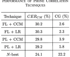
TABLE I
[image:5.612.93.236.76.193.2]PERFORMANCE OF PHONECORRELATION TECHNIQUES
Table I shows the performance of the techniques. Using a DP phone alignment (PL) of the two phone streams is superior to using a frame-level alignment and this is most effective when used in conjunction with the likelihood ratio (LR). Although the results from the techniques using a parallel phone recognizer are statistically significant, they are not practically significant and none comes close to the performance of the baseline -best technique. It was conjectured that if the acoustic models used in the two recognizers had some independence, these correlation techniques might perform better. We have some evidence that this is the case, but have not been able to confirm our results in time for publication.
V. METAMODELS
An attractive alternative to correlating the phone hypotheses from the recognizers is to construct word hypotheses from the phone recognizer output and compare these hypotheses with those output by the word recognizer. The alternative decoding is obtained from (5) by some segmentation algorithm which incor-porates the classification errors inherent in . Again, we would expect that where both sets of hypotheses decoded the same word in the same position, confidence in the correctness of that word would be high, given that the phoneme strings in the word decoding problem and in the phone recognition problem are from different “slices” of imposed by the respective Viterbi approximations. We first attempted to segment into words using a sliding window to isolate fixed-length subsequences of that might constitute fragments of a word, together with a confusion matrix that enabled us to account for possible errors in the phone decoding (a similar approach was used in [15]). However, these experiments convinced us that the large number of errors, especially insertions, in the phone recognizer stream made the segmentation problems quite unwieldy [10].
We therefore sought a method of accounting for likely errors in the phone recognizer stream whilst simultaneously segmenting it to form word hypotheses. A word recognition system effectively uses the Shannon “noisy channel” paradigm and this approach seemed to be also appropriate for our task. In a word recognition system, the HMMs model the mapping from sequences of “noisy” feature vectors to phonemes and the language model ensures that only legal sequences of phonemes (i.e., sequences of words) can be decoded. We use the same principle to decode the stream from the phone recognizer into words. However, the input to our word recognizer is the phone stream rather than a stream of acoustic feature vectors and
Fig. 1. Architecture of the metamodel of a phoneme.
our HMMs model the mapping between the “noisy” phone stream output by the phone recognizer and the reference transcription. As these discrete HMMs model the output from acoustic HMMs, we have termed them metamodels and the associated decoder a meta-recognizer.
Fig. 1 shows the architecture of a metamodel of a phoneme. The central state B of the metamodel for a phoneme models cor-rect decodings and substitutions of this phoneme made by the phone recognizer. The outer states, A and C, model (possibly multiple) insertions. A deletion is accommodated by the loop from input to output. Each state has a discrete probability dis-tribution over the phonemes associated with it. The metamodels are trained in the same manner as acoustic HMMs using em-bedded Baum-Welch re-estimation as follows:
1) Set the nonzero model transition probabilities to random values and seed the symbol distributions for each state equiprobably;
2) Use the reference transcriptions to concatenate the appro-priate sequence of phoneme metamodels for each training set utterance;
3) Use the decoded string for each utterance as training data and iterate re-estimation of the transition probabil-ities and distribution probabilprobabil-ities of the metamodels, using the Baum-Welch algorithm, until a suitable con-vergence criterion is reached.
Since the phone recognizer tends to produce insertions, there are always enough phones in any utterance to train the sequence of metamodels.
The language model is then used to compile the meta-recog-nizer network, which is identical to the network used in the word recognizer except that the nodes of the network are the appro-priate metamodels rather than the triphone acoustic models used by the word recognizer. At recognition time, the output of the phone recognizer is passed to the meta-recognizer to produce a set of hypotheses.2Dynamic programming is used to compare these hypotheses with the top hypothesis from the word recog-nizer and any word in the word recogrecog-nizer output that occurs more than times in the same position in the meta-recognizer output is marked as “C.” is determined experimentally and is in the range 1–5.
A. Metamodel Results
Table II compares the results for the metamodels confidence score with those obtained using -best. Note that a slightly smaller test-set from that used in Section IV-C was used here and the result for -best is slightly better than that quoted in
2When formulating word hypotheses using the meta-recognizer, the
TABLE II
PERFORMANCE OFMETAMODELSCM COMPAREDWITHN-BESTCM
TABLE III
ERRORPATTERN FORMETAMODELS ANDN-BESTCMS
TABLE IV
PERCENTAGE OFCORRECT ANDINCORRECTWORDS(COLUMNS3AND4) COMPAREDWITHPREDICTION OFTWOCONFIDENCEMEASURES
Section IV-C. Table III lists the number of words tagged cor-rectly or incorcor-rectly for each of the two confidence measures for the subset of words for which both measures gave a tag (some utterance files had to be discarded because the pruning thresh-olds for recognition were set too tightly). Table III shows, for example, that 1225 words were mistagged by -best, but cor-rectly tagged by the metamodel confidence measure etc. It is promising that only 463 of the 7221 words listed above were mistagged by both measures, indicating an upper bound of 6.4% tagging error over the baseline guessing measure (31% error) possible by some combination of the two features. A further breakdown of these figures in order to compare the performance of each tag-pair is given in Table IV. Table IV shows that when both confidence measures tag a word as correct, there is a 91.8% chance that the decoded word is correct. Conversely, when both tag incorrect, there is a 85.5% chance that the word is incorrect. Receiver operating curves for the -best and for the meta-model confidence methods are shown in Fig. 2.
B. Discussion
In Fig. 2, the lack of points for metamodel CMs at low false alarm levels is due to the fact that a metamodel CM cannot be computed for all words decoded by the word recognizer, be-cause not all the words in the word recognizer output string ap-pear in the word strings hypothesised by the metarecognizer. However, Fig. 2 shows that metamodel CMs are superior to -best CMs in regions where they operate together. In fact, the -best and metamodel methods are complementary, because it is not possible to operate the -best method at low levels of false acceptance, as there are some incorrect words that ap-pear in every hypothesis and hence have a confidence of 1.0 (a problem also noted in [16]). Hence, metamodels and -best
techniques can be used in combination to enable operation over the full range of false alarm/false acceptance tradeoff.
VI. USINGSEMANTIC INFORMATION AS AWAY OF
MEASURINGCONFIDENCE
An approach to confidence estimation that requires neither side information from the recognizer nor a parallel phonetic rec-ognizer must rely on either syntactical or semantical clues. Op-erating under the premise that correct recognition results should be more grammatical than incorrect results, Zhang and Rud-nicky have used a parser to extract confidence measures [17]. In this section, we describe the use of “semantic” knowledge to decide whether a decoded word is likely to be correct or not. Palmer and Ostendorf made some use of semantic knowledge in [5], where they found that knowing whether a word was part of a “location, organization or person phrase” was useful. Pao
et al. also used semantic information [18], but their technique
required hand-coding of the semantic categories of the vocabu-lary words, which ours does not.
Our technique was inspired by the observation that humans can identify some words that are incorrect in recognizer output on semantic grounds. Consider, for instance, a sentence decoded by our recognizer: “Exxon corporations said earlier this week that it replaced one hundred forty percent its violin gas pro-duction in nineteen eighty serve on.” Here, the word “violin” is clearly incorrect because it is not semantically related to the other content words in the sentence (the correct transcription is “oil and”). Of course, not all incorrectly decoded words can be so clearly identified on semantic grounds as in this example, but the occurrence of “semantic outliers” is not infrequent in rec-ognizer decodings (see Section VI-A for some numbers from our own recognizer). If decoded words could be tagged using this principle, no side information from the recognizer would be required. If side information is available, it can be used in conjunction with the semantic information, as this information will be independent of any information about the quality of the acoustic matching in the decoder and will also have a degree of independence from any measures derived from the decoder’s language model. In Section VI-F, we describe how these two sorts of information were combined to give an improved CM.
A. Preliminary Experiment
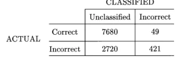
In a preliminary experiment, we investigated the viability of the idea of estimating confidence in the correctness of a decoded word using semantic information. We examined about 600 sen-tences decoded by our recognizer from the WSJCAM0 corpus and, without knowing the correct transcription, attempted to mark the words that we thought were incorrect on “semantic” grounds. This marking was done conservatively, i.e., only words that seemed to be clearly wrong because they were incongruous were tagged as . The confusion-matrix of our hand-marking is shown in Table V. Table V indicates that words
were tagged as out of the that were
Fig. 2. False acceptances versus false alarms at different thresholds. The dots are for the metamodel operating points and the pluses (+) are for N-best.
TABLE V
CONFUSION-MATRIX FORHAND-TAGGING OFWORDS ONSEMANTICGROUNDS
of emulating human performance by using a “semantic” crite-rion to identify incorrect words had the potential to identify only a small number of words, but with fairly high precision. The words we identified were all uncommon nouns or verbs that were incongruous: it would not be possible to identify incor-rectly decoded common words, such as function words. How-ever, nonfunction words, in most cases, bear more information and so are generally more important if a confidence measure is needed to support, e.g., a dialogue system.
B. Application of Latent Semantic Analysis
Latent semantic analysis (LSA) is a technique that has been in use for some years in the field of information retrieval and has latterly been applied in speech recognition [19]. It is not proposed to describe the theory of LSA in detail here—for an introduction, see, for example, [20]. LSA is a technique for as-sociating words that tend to co-occur within documents that are “semantically coherent” (examples of documents are entries in an encyclopaedia or stories in a newspaper). The assumption is
that words that tend to co-occur across documents are semanti-cally linked.
The essential idea behind LSA is to form a matrix of word/document co-occurrences and then to represent the row and column vectors of this very large matrix in a greatly reduced subspace using the technique of singular value decomposition (SVD). Because the matrix is very sparse and its rank is also much lower than its dimensionality, it is possible to represent the vectors in a low dimensional space with relatively small error. The key property of LSA is that words whose vectors are “close” in the reduced space correspond to semantically similar words (also, documents whose vectors are close in this space convey similar semantic meanings). It is this property that we have exploited for use in forming a confidence measure. By projecting the vocabulary words into the subspace, we can estimate a “semantic similarity” between any pair of words. These similarities can be used to provide an estimate of the likelihood of the words co-occurring within the same utterance, under the obvious assumption that the utterance and the training texts are homogeneous.
C. Application of LSA
Fig. 3. Distributions of “semantic similarities” for four words.
number of times word appears in document according to the technique described in [19]. In [19], entry ( ) of is defined as , where is a “global weight” for word and reflects the fact that words occur with different frequencies through documents and a local term that adjusts to take account of widely different values. There were 19 685 different words and 19 396 documents in the corpus. SVD of was done using the special MATLAB routine for sparse matrices . After some experimentation with different dimensionalities of reduced space, a reduced space dimensionality of 100 was used. Each word was then described by a 100-D vector and the “se-mantic similarity” between words and in the lexicon, , was computed as the cosine of the angle between the vectors, i.e.,
(11)
where is the 100-D vector associated with word . It
should be noted that and a high positive
value for indicates that the words and have a high semantic correlation.
Before proceeding to use these similarities for estimation of confidence measures, we were interested to examine their distri-butions for different words. The similarity between each word in the lexicon and all other words was computed to give a set of similarities for word . The mean similarity was computed for each word and the words were then ranked by their value of . It was noticeable that the words with high values of were predominantly (but not exclusively) function words. The words with the lowest values were, without excep-tion, rarely occurring nouns. Fig. 3 shows the distribution of the
for four words at different positions in the ranking. The implication of Fig. 3 is that broad distributions are associated with words that occur with many other words and hence have a broad range of semantic similarities, whereas the narrower dis-tributions centred on zero represent words that occur with only a small fixed set of words and hence have a semantic similarity close to zero to most other words in the lexicon.
It seemed possible that these “semantic similarities” were ac-tually simply a reflection of the fact that a word that occurred often in the training data would naturally co-occur with many other words and hence have a high mean similarity, whereas the reverse would be true for infrequently occurring words. How-ever, it was found that there was only a very weak correlation between the mean semantic similarity and the number of occur-rences (or the ranking of the number of occuroccur-rences) of a word ( for the latter case). For example, the word “proving” has a medium number of occurrences in the training-data (91, rank 6992) but a high mean semantic similarity of 0.385 (rank 165), which indicates that it co-occurs with a diverse collection of words. Conversely, “gas” has a high number of occurrences in the training-data (1946, rank 579), but a very low mean se-mantic similarity of 0.02 (rank 19 081), which indicates that it co-occurs only with a very specific set of other words.
D. Confidence Measures From LSA
We first attempted to identify words whose meaning and usage were not cognate with the other decoded words in the sentence by using the precomputed semantic similarities to compute the mean semantic similarity for each decoded word. Suppose that the sequence of words decoded from an input
the number of the decoded word in the sentence to the number of the same word in the lexicon. The mean semantic similarity for the th decoded word is
(12)
(Notice that if word is the same as word , , which increases the value of . In practice, only common function words usually reoccur in a decoding and as these words will be discarded after the applica-tion of a stop list (see Secapplica-tion VI-E), this effect does not cause a problem). We would expect to be low for semantically incorrect words and high for words that are cognate. However, is a poor indicator of semantically incorrect words. The reason for its poor performance is that most words have high similarities to function words and although a semantically incorrect word may have low similarities to other content words in the decoded sentence, these low similarities are masked by the “noise” from the higher similarities to decoded function words.
E. Using a Stop List to Eliminate Common Words
This result suggested that it was necessary to discard decoded words that had high mean semantic similarities to most other words in the lexicon, as these words had low semantic weight and contributed mainly noise to the value of for other words. Accordingly, we experimented with using a stop list [21] of decoded words whose value of was above a threshold . We then compute a confidence measure for each of the re-maining words. The confidence measures we experimented with were as follows.
1) as defined in (12);
2) , the mean rank of the semantic similarities to the de-coded word . was computed by finding the rank of each in the set of semantic similarities and then computing the mean;
3) , the probability that the set of semantic similarities between word and the other decoded words was generated from the distribution of similarities
(13)
where is a random variable whose distribution is estimated from , the set of semantic similarities for word . We ap-proximated the distributions shown in Fig. 3 by five component
Gaussian mixtures to estimate .
In practice, we found that all three of the above statistics gave very similar performance, with marginally the best. The effect of varying on the tagging accuracy of is shown in Table VI. In Table VI, is the error-rate of the recognizer on the retained words ( the “guessing” error-rate),
is the tagging error-rate when using the confidence-mea-sure and is the confidence gain. It is interesting that at first decreases, probably as more function-like words, which tend to have a higher error-rate than nonfunction words, are dis-carded. However, when 78% of words are discarded,
TABLE VI
EFFECT OFVARYING THETHRESHOLDL
begins to rise again and continues to rise. Examination of the words retained when shows a greatly increased pro-portion of single letter words, mostly “u,” “p,” and “s.” These words are almost always incorrect insertions by the decoder and hence the error-rate increases.
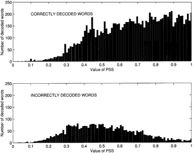
Table VI does not show the predicted increase in tagging ac-curacy when commonly co-occurring words are eliminated. An examination of the distribution of the values of was re-vealing. In Fig. 4, the values of for correctly (top) and in-correctly (bottom) decoded words are shown for i.e., with 53.6% of decoded words excluded. The histograms have a large overlap showing that is unable to separate these classes very effectively. However, it is interesting to examine the “tails” of the distributions. Our hypothesis is that a semantic confidence measure should be effective at identifying incorrect words and so we would expect to see a high probability of low values of for incorrect words and a low probability of low values of for correct words. In fact, Fig. 4 shows that the probabilities of low values of are very similar for both correct and incorrect words. However, high values of are significantly more probable for correct words than for incorrect words. Hence, is deriving its discrimination by identifying
correctly decoded words. Analysis revealed that the words
as-sociated with high values of were predominantly words that commonly occurred in the WSJ data (numbers, financial terms, etc.) that were highly cognate with each other. Inspection of the decoded words that had very low values of associ-ated with them showed that some of these were commonly oc-curring words that had been correctly decoded. The most likely reason that these common words have low semantic similarity to other decoded words is that they have not been seen to co-occur in the training corpus with them.
F. Combining Semantic and -Best Confidence Measures
Fig. 4. Distributions of values ofP SS for correct and incorrect words.
would be useful. We used the -best CM ( ) as described in Section IV-B to provide this. If we assume that and , the values of and for word , are independent esti-mates of the probability that word is correct, the product of these values ( ) gives a further estimate of this proba-bility. Fig. 5 shows receiver operating curves formed from the three CMs , and by varying the threshold above which words were classified as correct (N.B. this was run on all decoded utterances). Fig. 5 shows that (squares) is generally a poor indicator of the status of a decoded word: if all decoded words are examined, its performance is no better than chance, but as the proportion of decoded words examined drops, its accuracy increases to close to 100%. (crosses) is better for high values of recall, but the maximum precision is ca-pable of is 87.5% at a recall of about 50%. The single point to the left of this point is made from the values of that are exactly 1.0 (i.e., words that occur in all top 100 decodings) and the proportion of such words that are actually correct is about 85.5%. When is combined with to form
(asterisks), performance with high recall is slightly better than alone retains the ability of to give high pre-cision for low recall. This is useful if it is desired to identify a small number of decoded words as correct with a high confi-dence.
G. Discussion
Using information about how well a decoded word relates semantically to the other decoded words in an utterance can provide useful information about whether the word is correct.
This information is largely independent of information derived from a “side information” based confidence measure, such as -best and hence complements the latter. Although our orig-inal idea was that a semantically based CM would be able to identify incorrectly decoded words that were not cognate with the other decoded words in an utterance, we found unexpectedly that it was better at predicting correctly rather than incorrectly decoded words. The ability of the technique to identify correctly decoded words seems to be due to the presence of a set of com-monly occurring content words in the WSJ data that are highly cognate (e.g., numbers, financial terms). The technique was ca-pable of identifying incongruous words successfully (such as the example quoted in Section VI), but was unable to discrimi-nate between these words and correctly decoded common words occurring in a previously unseen context. It was clear from the preliminary experiment that this approach would only ever be capable of giving confidence measures for infrequently occur-ring content words and future work will include integration of word probability measures with the semantic measures to en-hance this ability.
VII. SUMMARY ANDDISCUSSION
Fig. 5. Recall/precision curves forP SS, NB, and NBP SS.
TABLE VII
SUMMARY OFPERFORMANCE OF THETECHNIQUESDISCUSSED IN THEPAPER
have examined ways of using two extra sources of information: a phone-loop recognizer working in parallel with the word rec-ognizer and a “semantic distance” between the words present in the word recognizer output. Table VII summarizes the perfor-mance of the techniques discussed in the paper. In Section III, we developed some theory that gives an approach to using the output of a phone recognizer in tandem with the output from a word recognizer to derive confidence measures for the words output by the word recognizer. This theory was utilized in Sec-tion IV in a technique called “phone correlaSec-tion.” Phone correla-tion gives a small improvement in confidence over guessing, but Table VII shows that using a phone-loop recognizer to construct “metamodels” has much more benefit. Section V extended the ideas of Section III to develop the use of metamodels, in which putative word strings are constructed from the output of the phone recognizer. By comparing these strings with the word strings produced by the word recognizer a confidence measure can be produced. This is a more complex technique than either
-best or phone correlation that offers substantially better per-formance than both. It could also be used effectively in tandem with the -best technique if -best information is available. Metamodels attempt to capture the mapping from the output of a phone recognizer to the true transcription and as such may find application in other areas of speech recognition (in pronuncia-tion modeling, for instance).
Section VI introduced an approach that was motivated by the idea that words decoded by the recognizer that are semantically “distant” from the other decoded words are more likely to be in-correct. The semantically based technique has the advantage of requiring no side information at all from the recognizer: on its own, it is a weak indicator of confidence, but when combined with -best, it produced a very useful gain in the low recall/high precision region. -best performs poorly in this region because there are a significant number of incorrect utterances that have an -best “score” of 100%. We speculate that the semantically based technique would be most effective when used in an ap-plication that has several domains that are fairly independent of each other, but which uses a single vocabulary and language model.
We are currently in the process of testing the effectiveness of all these techniques and comparing them with conventional techniques, on a real dialogue system.
REFERENCES
[1] L. Chase, “Word and acoustic confidence annotation for large vocabu-lary speech recognition,” in Proc. 5th Eur. Conf. Speech Communication
[2] L. Gillick, Y. Ito, and J. Young, “A probabilistic approach to confidence estimation and evaluation,” in Proc. IEEE Conf. Acoustics, Speech,
Signal-Processing, Apr. 1997.
[3] T. Schaaf and T. Kemp, “Confidence measures for spontaneous speech recognition,” in Proc. IEEE Conf. Acoustics, Speech, Signal-Processing, Apr. 1997.
[4] S. J. Cox and R. C. Rose, “Confidence measures for the SWITCH-BOARD database,” in Proc. IEEE Conf. Acoustics, Speech,
Signal-Pro-cessing, 1996, pp. 511–515.
[5] D. D. Palmer and M. Ostendorf, “Improved word confidence estimation using long range features,” in Proc. 7th Eur. Conf. Speech
Communica-tion and Technology, Sept. 2001.
[6] A. Asadi, R. Schwartz, and J. Makhoul, “Automatic detection of new words in a large vocabulary speech recognition system,” in Proc. IEEE
Conf. Acoustics, Speech, Signal-Processing, 1990, pp. 125–128.
[7] M. C. Benitez et al., “Word verification using confidence measures in speech recognition,” in Proc. 5th Int. Conf. Speech Communication and
Technology, Nov. 1998, pp. 1082–1085.
[8] T. Robinson et al., “WSJCAM0: A British English speech corpus for large vocabulary continuous speech recognition,” in Proc. IEEE Conf.
Acoustics, Speech, Signal-Processing, 1995, pp. 81–84.
[9] J. Jansen, J. Odell, D. Ollason, and P. Woodland, The HTK Book: En-tropic Res. Labs., Inc., 1996.
[10] S. J. Cox and S. Dasmahapatra, “A high-level approach to confidence estimation in speech recognition,” in Proc. 6th Eur. Conf. Speech
Com-munication and Technology, Sept. 1999, pp. 41–44.
[11] S. Dasmahapatra and S. J. Cox, “Meta-models for confidence estimation in speech recognition,” in Proc. IEEE Conf. Acoustics, Speech,
Signal-Processing, June 2000.
[12] Z. Chair and P. Varshney, “Optimal data fusion in multiple sensor detec-tion,” IEEE Trans. Aerosp. Electron. Syst., vol. 22, no. 1, pp. 98–101, 1986.
[13] L. Chase, “Error-Responsive Feedback Mechanisms for Speech Recog-nizers,” Ph.D., Carnegie Mellon Univ., Pittsburgh, PA, 1997. [14] M. Weintraub et al., “Neural-network based measures of confidence for
word recognition,” in Proc. IEEE Conf. Acoustics, Speech, Signal
Pro-cessing, Apr. 1997.
[15] R. R. Sarukkai and D. H. Ballard, “Phonetic set indexing for fast lexical access,” IEEE Trans. Pattern Anal. Machine Intell., vol. 20, pp. 78–82, Jan. 1998.
[16] F. Wessel, S. Schlüter, K. Macherey, and H. Ney, “Confidence measures for large vocabulary speech recognition,” IEEE Trans. Speech Audio
Processing, vol. 9, pp. 288–298, Mar. 2001.
[17] R. Zhang and A. I. Rudnicky, “Word level confidence annotation using combinations of features,” in Proc. 7th Eur. Conf. Speech
Communica-tion and Technology, Sept. 2001.
[18] C. Pao, P. Schmid, and J. Glass, “Confidence scoring for speech under-standing systems,” in Proc. 5th Int. Conf. Spoken Language Processing, Dec. 1998.
[19] J. R. Bellegarda, “A multispan language modeling framework for large vocabulary speech recognition,” IEEE Trans. Speech Audio Processing, vol. 6, pp. 456–467, Sept. 1998.
[20] T. K. Landauer and S. T. Dumais, “A solution to Plato’s problem: Rep-resentation of knowledge,” Psychol. Rev., vol. 104, pp. 211–240, 1997. [21] C. D. Manning and H. Schutze, Foundations of Statistical Natural
Lan-guage Processing. Cambridge, MA: MIT Press, 1999.
Stephen Cox (M’00) received the B.Sc. and M.Phil. degrees in physics and music from Reading Univer-sity, Reading, U.K., and the Ph.D. degree in speech recognition from the University of East Anglia, Nor-folk, U.K.
His research interests are in speech processing, especially recognition, and pattern recognition. He joined British Telecom Research Laboratories (BTRL) in 1984 where he was concerned with assessment of speech recognition algorithms. From 1987 to 1989, he worked on rapid speaker adaptation at the Speech Research Unit at DERA, Great Malvern, U.K. He returned to BTRL in 1989 as Head of a group developing robust speech recognition algorithms for use over the telephone network. He was appointed Lecturer in Electronic Systems Engineering at the University of East Anglia in 1991 and Senior Lecturer in 1998. From July to December 1994, he was a Visiting Scientist in the Speech Research Group at AT&T Bell Labs, Murray Hill, NJ, and during the autumn of 2000, was Visiting Scientist at Nuance Communications, Menlo Park, CA. He is the author of more than 50 papers in the fields of speech and pattern processing.
Dr. Cox is Chairman of the U.K. Institute of Acoustics Speech Group.
Srinandan Dasmahapatra received the B.Sc. (Hons.) degree in physics from St. Xavier’s College, Calcutta University, India, and the Ph.D. degree in physics from the State University of New York at Stony Brook.