A Fuzzy-Neural Adaptive Iterative Learning Control for Freeway Traffic Flow Systems

A Fuzzy-Neural Adaptive Iterative Learning

Control for Freeway Traffic Flow Systems

Ying-Chung Wang, Chiang-Ju Chien, and Chun-Hung Wang

Abstract—In this paper, a fuzzy-neural adaptive iterative learning control (AILC) is proposed for traffic flow systems of a single lane freeway with random bounded off-ramp traffic volumes. It is assumed that the system dynamic functions and input gains are unknown for controller design. An adaptive fuzzy neural network (FNN) controller and an adaptive robust controller are applied to compensate for the unknown system nonlinearity and input gain respectively. On the other hand, to deal with the disturbance from random bounded off-ramp traffic volumes, a dead zone like auxiliary error with the time-varying boundary layer is introduced as a bounding parameter. This proposed auxiliary error is also utilized for the construction of adaptive laws without using the bound of the input gain for all the adaptation parameters. The traffic density tracking error is shown to converge along the axis of learning iteration to a residual set whose level of magnitude depends on the width of boundary layer.

Index Terms—fuzzy neural network, adaptive iterative learn-ing control, traffic flow systems, random bounded off-ramp traffic volumes.

I. INTRODUCTION

I

T is well-known that the traffic congestions on freeways are one of the main traffic problems in Taiwan. The freeway ramp metering [1] is one of the most typical control approaches to adjust the traffic flow of freeway. Besides, the PID-type control in [2], neural network control in [3], and optimal control in [4] are also some popular control method-ologies in the research field of freeway ramp metering. The authors in [1], which is a good review of recent freeway ramp metering, have commented that the freeway ramp metering can be further divided into three classes of control strategies: 1. fixed-time ramp metering control, 2. local ramp metering control, 3. system ramp metering control. In the local ramp metering control strategies, ALINEA local ramp metering has been widely applied in the freeway traffic flow systems for a long period of time. In fact, ALINEA local ramp metering is a traditional PI-type controller which is not suitable for dealing with highly nonlinear systems with uncertainties. In addition, since very few strict mathematical analysis can be applied to design the controller gains of ALINEA local ramp metering, the system stability can not be guaranteed by ALINEA local ramp metering.

On the other hand, high repeatabilities often exist in the freeway traffic flow systems. For example, traffic congestions on the same freeway always repetitively appear in the same peak time interval from 7 to 9 AM every Monday. Unfor-tunately, the aforementioned freeway ramp metering control strategies are typical time-domain control approaches which

Ying-Chung Wang is with the Department of Electronic Engineering, Huafan University, New Taipei City, Taiwan e-mail: ([email protected]).

Chiang-Ju Chien, and Chun-Hung Wang are with the Department of Electronic Engineering, Huafan University, New Taipei City, Taiwan.

do not consider the repetitive characteristics of freeway traffic flow systems for the design of ramp metering controller. This implies that these existing freeway ramp metering control approaches are not suitable to perform a repeated traffic control task for traffic flow systems. Recently, traditional discrete iterative learning control (ILC) schemes have been successfully applied for freeway traffic flow systems [5], [6], [7] with a repetitive task over a finite time interval. However, it is assumed that the system nonlinearities satisfy global Lipschitz continuous condition.

In this paper, the repetitive tracking control problem of traffic flow systems of a single lane freeway with random bounded off-ramp traffic volumes is studied. We consider a more general case in the sense that the system nonlinearities and system parameters are allowed to be unknown. An adaptive fuzzy neural network (FNN) controller and an adaptive robust controller are applied to compensate for the unknown system nonlinearity and input gain respectively. On the other hand, to deal with the disturbance from random bounded off-ramp traffic volumes, a dead zone like auxiliary error with the time-varying boundary layer is introduced as a bounding parameter. This proposed auxiliary error is also utilized for the construction of adaptive laws without using the bound of the input gain for all the adaptation parameters. The traffic density tracking error is shown to converge along the axis of learning iteration to a residual set whose level of magnitude depends on the width of boundary layer.

This paper is organized as follows. In section II, a problem formulation is given. The discrete AILC is then presented in section III. Based on the proposed AILC and a derived traffic density tracking error model, the analysis of closed-loop stability and learning performance will be studied extensively in Section IV. A simulation example is given in Section V to demonstrate the effectiveness of the proposed learning controller. Finally a conclusion is made in Section VI.

II. PROBLEMFORMULATION

In this paper, we consider an uncertain traffic flow system [8] for a single lane freeway with n sections which can perform a given task repeatedly over a finite time sequence t ∈ {0,1,2,· · ·, N}. The traffic flow system for a single lane freeway with one on-ramp and one off-ramp in the ith section,i= 1,· · ·, nis represented as follows:

ρj_i(t+ 1) = fi(qij−1(t), ρji(t), qji(t)) +

T Li

³

rj_i(t)−sj_i(t)´

q_ij(t) = ρj_i(t)ν_ij(t)

ith section (in vehicles per lane per kilometer), ν_ij(t) ∈ R is the space mean speed in theith section (in kilometers per hour),qj_i(t)∈ Ris the traffic flow leaving theith section and entering thei+ 1th section (in vehicles per hour),r_ij(t)∈ R is the on-ramp traffic volume in the ith section (in vehicles per hour), sj_i(t) ∈ R is the off-ramp traffic volume of the ith section (in vehicles per hour) considered to be an un-known random bounded disturbance,fi(qji−1(t), ρji(t), qij(t))

and gi(νij−1(t), ρji(t), νij(t), ρji+1(t+ 1)) are unknown real continuous nonlinear functions of ν_ij₋₁(t), q_ij₋₁(t), ρj_i(t), νij(t),qij(t),ρji+1(t+1). Based on (1), theith freeway traffic flow subsystem can be rewritten as follows:

ρj_i(t+ 1)

= fi(ρji−1(t), νij−1(t), ρji(t), νij(t)) +

T Li

³

r_ij(t)−sj_i(t)´

(2)

Now, given a specified iteration-varying desired traffic den-sity trajectory of the ith freeway traffic flow subsystem ρj_di(t) ∈ R, t ∈ {0,1,2,· · ·, N + 1}, the control objective is to design an AILC to adjust the on-ramp traffic volume rj_i(t) such that the traffic density ρj_i(t) can follow ρj_di(t) as close as possible∀t∈ {1,2,· · ·, N+ 1}when iterationj approaches infinity. In order to achieve this control objective, some assumptions on the freeway traffic flow system and desired traffic density trajectories are given as follows:

(A1) The freeway traffic flow system is a relaxed system whose on-ramp traffic volumes rj_i(t), traffic densities ρj_i(t), space mean speeds ν_ij(t) and traffic flowsq_ij(t)

are related by ρj_i(t) = 0, ν_ij(t) = 0 and qj_i(t) = 0, t <0.

(A2) The traffic flow rate entering the first section isqj₀(t)and the mean speed of the traffic entering the first section is assumed to be the mean speed in the first section, i.e., ν₀j(t) =ν₁j(t). We also assume that the mean speed and traffic density of the traffic exiting the n+ 1th section are assumed to be those innth section, i.e.,νnj+1(t) = νj

n(t), ρjn+1(t) = ρjn(t). The boundary conditions can

be defined as ρj₀(t)≡ q j

0(t)

νj

1(t)

,ν₀j(t)≡ν₁j(t),ρj_n+1(t)≡ ρj

n(t)andνjn+1(t)≡νnj(t), respectively.

(A3) There exists a positive unknown constantsU such that

|sj_i(t)| ≤sU for allt∈ {0,1,· · ·, N},j≥1.

(A4) There exists a positive known constant ρU_d such that |ρj_di(t)| ≤ρU

d for allt∈ {0,1,· · ·, N+ 1},j≥1.

(A5) Let traffic density tracking errors be defined asej_i(t) = ρj_i(t)−ρj_di(t). The initial traffic density tracking errors at each iteration ej_i(0)are bounded.

III. THEFUZZY-NEURALAILC

In order to find the approach for controller design later, we first derive the traffic density tracking error equation as:

ej_i(t+ 1) = fi(ρji−1(t), νij−1(t), ρji(t), νij(t)) +

T Li

rj_i(t)

− T Lis

j i(t)−ρ

j

di(t+ 1) (3)

In order to overcome the design problem due to un-known nonlinear function fi(ρji−1(t), νij−1(t), ρji(t), νij(t))

of the ith traffic flow subsystem, we apply the univer-sal approximation technique to construct the basic struc-ture of our AILC. An MIMO FNN [9] described by Θj(t)>_Φ(ρj

i−1(t), νij−1(t), ρji(t), νij(t)) is utilized as the

approximators of fi(ρji−1(t), νij−1(t), ρji(t), νij(t)), i = 1,2,· · ·, n. Here Φ(ρj_i−1(t), ν_ij₋₁(t), ρj_i(t), ν_ij(t))∈ RM×1 is the radial basis function vector in the rule layer of the MIMO FNN with M being the number of rules, Θj_{(t) ∈}

RM×n _{is the output weight matrix of the output layer with}

Θ_ij(t)∈ RM×1 _{being theith output weight vector. In other} words, Θ_ij(t)>_Φ(ρj

i−1(t), νij−1(t), ρji(t), νij(t)) denotes the

ith output of the MIMO FNN. In this work, we use the ith output of the MIMO FNN to uniformly approximate the nonlinear functionfi(ρji−1(t), ν

j i−1(t), ρ

j i(t), ν

j

i(t))of theith

traffic flow subsystem on a compact set Ac ⊂ R4×1. An

important aspect of the above approximation property is that there exist an optimal parameter vectorΘ∗

i for theith output

of the MIMO FNN such that the function approximation error ²i(ρji−1(t), νij−1(t), ρji(t), νij(t)) between the ith

out-put of the optimal FNN Θ_i∗>Φi(t) and nonlinear function

fi(ρji−1(t), νij−1(t), ρji(t), νij(t)) can be bounded by

pre-scribed constants²∗_i on the compact setAc. More precisely, if

we defineΦj(t)≡Φi(ρji−1(t), νij−1(t), ρji(t), νij(t))and the

²j_i(t)≡²i(ρji−1(t), νij−1(t), ρji(t), νij(t)) for simplicity, then

we have fi(ρji−1(t), νij−1(t), ρji(t), νij(t)) = Θi∗>Φi(t) +

²j_i(t) and |²j_i(t)| ≤ ²∗

i, ∀(ρji−1(t), νij−1(t), ρji(t), νij(t)) ∈

Ac.

Based on the traffic density tracking error equation in (3) and theith output of the MIMO FNN, we propose the fuzzy-neural AILC for the ith freeway traffic flow subsystem (2) as:

rj_i(t) = ψ j i(t)

δ+ψ_ij(t)2

h

−Θ_ij(t)>_Φj_{(t) +ρ}j di(t+ 1)

i

(4)

whereδ >0. To further see the insight of the proposed AILC (4), we substitute (4) into (3) and find that

ej_i(t+ 1)

= fi(ρji−1(t), νij−1(t), ρij(t), νij(t))−Θij(t)>Φj(t)

+ µ

T Li −ψ

j i(t)

¶

r_ij(t) +Θ_ij(t)>_Φj_(t)−ρj di(t+ 1)

+ ψ

j i(t)2

δ+ψj_i(t)2

h

−Θ_ij(t)>Φj(t) +ρj_di(t+ 1) i

− T Lis

j i(t)

= ¡Θi∗−Θij(t) ¢>

Φj(t) + µ

T Li −ψ

j i(t)

¶

r_ij(t) +δj_Li(t)

(5)

where

δj_Li(t) = ²j_i(t)− T Li

sj_i(t)

+ δ

δ+ψ_ij(t)2

h

Θ_ij(t)>Φj(t)−ρj_di(t+ 1) i

(6)

It is clear thatδ_Lij (t)can be shown to be bounded byΘ_ij(t)

as follows:

|δ_Lij (t)| ≤

¯ ¯ ¯ ¯ ¯

δ δ+ψ_ij(t)2

h

Θ_ij(t)>_Φj_(t)−ρj di(t+ 1)

i¯¯ ¯ ¯ ¯

+ ¯ ¯ ¯²j_i(t)

¯ ¯ ¯+

¯ ¯ ¯ ¯_LT_isji(t)

≤ θ∗

i ¡¯_¯

Θ_ij(t)¯¯+ 1¢ (7)

where θ∗

i, i = 1,2,· · ·, n are some unknown positive

constants. In order to overcome the uncertaintyδ_Lij (t)in (7), we now define an auxiliary errorej_φi(t+ 1)of theith traffic flow subsystem as

ej_φi(t+ 1) =ej_i(t+ 1)−φj_i(t+ 1)sat Ã

ej_i(t+ 1)

φj_i(t+ 1) !

(8)

for t ∈ {0,1,2,· · ·, N}. We don’t define ej_φi(0) of the ith traffic flow subsystem since it will not be utilized in our design of controller and adaptive laws. In (8), sat is the saturation function defined as in [10] and φj_i(t+ 1) is the width of the time-varying boundary layer for the ith traffic flow subsystem which is to be designed later. It is noted that ej_φi(t+ 1)of theith traffic flow subsystem which can be defined as in [10] and it can be easily shown that ej_φi(t+ 1)sat

³ ej

i(t+1) φj

i(t+1)

´

=|ej_φi(t+ 1)|,∀j≥1.

Next, the time-varying boundary layer for the ith traffic flow subsystem will be designed as follows:

φj_i(t+ 1) =θj_i(t)¡¯¯Θ_ij(t)¯¯+ 1¢ (9)

whereθj_i(t)is a parameter of theith boundary to be updated later. In this AILC, Θ_ij(t), ψ_ij(t) in (4) and θ_ij(t) in (9) are designed to compensate the unknown optimal consequent parameter vectors Θ∗

i, input gains LTi andθ

∗

i, respectively.

The adaptive laws forΘ_ij(t),ψj_i(t)andθj_i(t)at (next)j+1th iteration are given as follows :

Θ_ij+1(t)

= Θ_ij(t) + β1e j

φi(t+ 1)Φj(t) 1 +¯¯Φj_(t)¯¯2₊¯¯_rj

i(t) ¯ ¯2

+¡¯¯Θ_ij(t)¯¯+ 1¢2

(10) ψ_ij+1(t)

= ψj_i(t) + β2e j

φi(t+ 1)r j i(t) 1 +¯¯Φj_(t)¯¯2₊¯¯_rj

i(t) ¯ ¯2

+¡¯¯Θ_ij(t)¯¯+ 1¢2

(11) θj_i+1(t)

= θ_ij(t) + β3|e j

φi(t+ 1)| ¡¯_¯

Θ_ij(t)¯¯+ 1¢ 1 +¯¯Φj_(t)¯¯2₊¯¯_rj

i(t) ¯ ¯2

+¡¯¯Θ_ij(t)¯¯+ 1¢2

(12)

for t ∈ {0,1,2,· · ·, N}, where β1, β2, β3 > 0 are the adaptation gains. For the first iteration, we set Θ1

i(t) =Θi1

and ψ1

i(t) = ψi1 to be any constant vector and constant,

respectively. θ1

i(t) = θ1i > 0 ∀t ∈ {0,1,2,· · ·, N} to be

a small fixed value ∀t ∈ {0,1,2,· · ·, N}. It is noted that θ_ij(t) >0,∀t ∈ {0,1,2,· · ·, N} and ∀j ≥1. Furthermore, we will choose ψ1_{(t) =ψ}1 _{as a nonzero constant in order} to prevent the controller (4) from being a zero input in the beginning of the learning process.

IV. ANALYSIS OFSTABILITY ANDCONVERGENCE

In this section, we will analyze the closed loop stability and learning convergence. At first, define the parameter errors as Θe_ij(t) = Θ_ij(t)−Θ∗

i, θegj(t) = ψij(t)− LTi,

e

θj_i(t) =

θj_i(t)−θ∗

i. Then it is easy to show, by subtracting the optimal

control gains on both sides of (10)-(12), that

e

Θ_ij+1(t)

= Θe_ij(t) + β1e j

φi(t+ 1)Φj(t) 1 +¯¯Φj_(t)¯¯2₊¯¯_rj

i(t) ¯ ¯2

+¡¯¯Θ_ij(t)¯¯+ 1¢2

(13)

e

ψj_i+1(t)

= ψe_ij(t) + β2e j

φi(t+ 1)rji(t) 1 +¯¯Φj_(t)¯¯2₊¯¯_rj

i(t) ¯ ¯2

+¡¯¯Θij(t) ¯ ¯_{+ 1}¢2

(14)

e

θ_ij+1(t)

= eθj_i(t) + β3|e j

φi(t+ 1)| ¡¯

¯_Θj i(t)

¯ ¯_{+ 1}¢

1 +¯¯Φj_(t)¯¯2₊¯¯_rj i(t)

¯ ¯2

+¡¯¯Θ_ij(t)¯¯+ 1¢2

(15)

Now we are ready to state the main results in the following theorem.

Main Theorem. Consider the traffic flow systems in (1)

satisfying the assumptions (A1)-(A5). If the fuzzy-neural AILC is designed as in (4), (8), (10), (11) and (12) with adaptive laws (10), (11) and (12) for the ith freeway traffic flow subsystem and the following condition can be satisfied:

2−β1−β2−β3>0, (16)

then the tracking performance and system stability will be guaranteed as follows:

(t1) The adjustable parametersΘ_ij(t),ψ_ij(t),θ_ij(t)and con-trol inputsrj_i(t)are bounded∀t∈ {0,1,· · ·, N}, j≥1. (t2) The auxiliary traffic density tracking errorsej_φi(t+1)are bounded∀t∈ {0,1,· · ·, N}, j≥1andlimj→∞ej_φi(t+

1) = 0,∀t∈ {0,1,· · ·, N}

(t3) The traffic density tracking errorej_i(t+ 1)are bounded ∀t ∈ {0,1,· · ·, N}, j ≥1 and limj→∞|eji(t+ 1)| ≤

θ∞

i (t) (|Θi∞(t)|+ 1),∀t∈ {0,1,· · ·, N} Proof :

(t1) Define the cost functions of performance as follows

V_ij(t) = 1

β1Θe

j i(t)>Θe

j i(t) +

1

β2ψe

j i(t)2+

1

β3θe

j i(t)2

Then, the difference between Vj+1_{(t) and V}j_{(t) can be}

derived as follows :

V_ij+1(t)−V_ij(t)

= 1

β1

³ e

Θ_ij+1(t)>Θe_ij+1(t)−Θe_ij(t)>Θe_ij(t) ´

+1

β2

³ e

ψ_ij+1(t)2_−ψej i(t)2

´

+1

β3

³ e

θj_i+1(t)2−θe_ij(t)2 ´

= 2e

j

φi(t+ 1)Θe j

i(t)>Φj(t) 1 +¯¯Φj_(t)¯¯2₊¯¯_rj

i(t) ¯ ¯2

+¡¯¯Θ_ij(t)¯¯+ 1¢2

+ β1e

j

φi(t+ 1)2 ¯ ¯_Φj_(t)¯_¯2 ³

1 +¯¯Φj_(t)¯¯2₊¯¯_rj i(t)

¯ ¯2

+ 2e j

φi(t+ 1)ψeji(t)rij(t) 1 +¯¯Φj_(t)¯¯2₊¯¯_rj

i(t) ¯ ¯2

+¡¯¯Θ_ij(t)¯¯+ 1¢2

+ β2e

j

φi(t+ 1)2 ¯ ¯ ¯rj_i(t)

¯ ¯ ¯2 ³

1 +¯¯Φj_(t)¯¯2₊¯¯_rj i(t)

¯ ¯2

+¡¯¯Θ_ij(t)¯¯+ 1¢2´2

+ 2|e

j

φi(t+ 1)|θe j i(t)

¡¯ ¯_Θj

i(t) ¯ ¯_{+ 1}¢

1 +¯¯Φj_(t)¯¯2₊¯¯_rj i(t)

¯ ¯2

+¡¯¯Θ_ij(t)¯¯+ 1¢2

+ β3e

j

φi(t+ 1)2 ¡¯

¯_Θj i(t)

¯ ¯_{+ 1}¢2

³

1 +¯¯Φj_(t)¯¯2₊¯¯_rj i(t)

¯ ¯2

+¡¯¯Θ_ij(t)¯¯+ 1¢2´2

(17)

Since (5) can be rewritten as

e

Θ_ij(t)>_Φj_{(t) +ψe}j

i(t)rji(t) =−eji(t+ 1) +δLij (t) (18)

This implies that

ej_φi(t+ 1)Θe_ij(t)>Φj(t) +ej_φi(t+ 1)ψej_i(t)rj_i(t) = −ej_i(t+ 1)ej_φi(t+ 1) +ej_φi(t+ 1)δj_Li(t) (19)

Substituting (19) into (17), we have

V_ij+1(t)−V_ij(t)

≤ −2e

j

i(t+ 1)ejφi(t+ 1) + 2ejφi(t+ 1)δLij (t) 1 +¯¯Φj_(t)¯¯2₊¯¯_rj

i(t) ¯ ¯2

+¡¯¯Θ_ij(t)¯¯+ 1¢2

+ β1e

j

φi(t+ 1)2 ¯ ¯_Φj_(t)¯_¯2 ³

1 +¯¯Φj_(t)¯¯2₊¯¯_rj i(t)

¯ ¯2

+¡¯¯Θ_ij(t)¯¯+ 1¢2 ´2

+ β2e

j

φi(t+ 1)2 ¯ ¯_rj

i(t) ¯ ¯2

³

1 +¯¯Φj_(t)¯¯2₊¯¯_rj i(t)

¯ ¯2

+¡¯¯Θ_ij(t)¯¯+ 1¢2 ´2

+ 2|e

j

φi(t+ 1)|θe j i(t)

¡¯_¯

Θ_ij(t)¯¯+ 1¢ 1 +¯¯Φj_(t)¯¯2₊¯¯_rj

i(t) ¯ ¯2

+¡¯¯Θ_ij(t)¯¯+ 1¢2

+ β3e

j

φi(t+ 1)2 ¡¯_¯

Θ_ij(t)¯¯+ 1¢2 ³

1 +¯¯Φj_(t)¯¯2₊¯¯_rj i(t)

¯ ¯2

+¡¯¯Θ_ij(t)¯¯+ 1¢2 ´2

(20)

If we substitue (8) into (20) and using the fact that|δj_Li(t)| ≤ θ∗

i ¡¯

¯_Θj i(t)

¯

¯_{+ 1}¢_{in (7), we can derive that}

V_ij+1(t)−V_ij(t)

≤ −2e

j

φi(t+ 1)2 1 +¯¯Φj_(t)¯¯2₊¯¯_rj

i(t) ¯ ¯2

+¡¯¯Θ_ij(t)¯¯+ 1¢2

− 2|e

j

φi(t+ 1)|θ j i(t)

¡¯ ¯_Θj

i(t) ¯ ¯_{+ 1}¢

1 +¯¯Φj_(t)¯¯2₊¯¯_rj i(t)

¯ ¯2

+¡¯¯Θ_ij(t)¯¯+ 1¢2

+ 2|e

j

φi(t+ 1)|θi∗ ¡¯_¯

Θ_ij(t)¯¯+ 1¢ 1 +¯¯Φj_(t)¯¯2₊¯¯_rj

i(t) ¯ ¯2

+¡¯¯Θ_ij(t)¯¯+ 1¢2

+ 2|e

j

φi(t+ 1)|θe j i(t)

¡¯_¯

Θ_ij(t)¯¯+ 1¢ 1 +¯¯Φj_(t)¯¯2₊¯¯_rj

i(t) ¯ ¯2

+¡¯¯Θ_ij(t)¯¯+ 1¢2

+ β1e

j

φi(t+ 1)2 ¯ ¯_Φj_(t)¯_¯2 ³

1 +¯¯Φj_(t)¯¯2₊¯¯_rj i(t)

¯ ¯2

+¡¯¯Θ_ij(t)¯¯+ 1¢2 ´2

+ β2e

j

φi(t+ 1)2 ¯ ¯ ¯r_ij(t)

¯ ¯ ¯2 ³

1 +¯¯Φj_(t)¯¯2₊¯¯_rj i(t)

¯ ¯2

+¡¯¯Θ_ij(t)¯¯+ 1¢2 ´2

+ β3e

j

φi(t+ 1)2 ³

1 +¯¯Φj_(t)¯¯2₊¯¯_rj i(t)

¯ ¯2

+¡¯¯Θ_ij(t)¯¯+ 1¢2 ´2

≤ −(2−β1−β2−β3)e

j

φi(t+ 1)2 1 +¯¯Φj_(t)¯¯2₊¯¯_rj

i(t) ¯ ¯2

+¡¯¯Θ_ij(t)¯¯+ 1¢2 (21)

If we chooseβ1,β2andβ3such thatk≡2−β1−β2−β3>0, then we have

V_ij+1(t)−V_ij(t)

≤ −ke

j

φi(t+ 1)2 1 +¯¯Φj_(t)¯¯2₊¯¯_rj

i(t) ¯ ¯2

+¡¯¯Θ_ij(t)¯¯+ 1¢2 ≤0(22)

forj≥1. SinceV1_{(t)is bounded∀t∈ {0,1,2,· · ·, N}due} toΘe1(t) =Θ1(t)−Θ_i∗=Θ_i1−Θ_i∗,ψe1(t) =ψ1(t)−_LT

i = ψ1₋ T

Li and θe 1

i(t) = θ1i(t)−θi∗ = θ1i −θi∗ are bounded

∀t∈ {0,1,2,· · ·, N}, we conclude that from (22) thatVj(t), and henceΘe_ij(t),ψej_i(t)andθej_i(t), are bounded∀j≥1. The boundedness of rj_i(t) is then guaranteed by using (4). This proves (t1) of the main theorem.

(t2) By summing (22) from1 toj leads to

V_ij(t)≤V1

i (t)− j X

i=1

−kej_φi(t+ 1)2

1 +¯¯Φj_(t)¯¯2₊¯¯_rj i(t)

¯ ¯2

+¡¯¯Θ_ij(t)¯¯+ 1¢2

SinceV_i1(t)is bounded andVj(t)must be nonnegative, we have

lim j→∞

ej_φi(t+ 1)2

1 +¯¯Φj_(t)¯¯2₊¯¯_rj i(t)

¯ ¯2

+¡¯¯Θ_ij(t)¯¯+ 1¢2 = 0

∀t ∈ {0,1,2,· · ·, N}. Since 1 + ¯¯Φj_(t)¯_¯2 ₊ ¯_¯rj i(t)

¯ ¯2

+ ¡¯_¯

Θ_ij(t)¯¯ + 1¢2 are bounded for all j ≥ 1 and t ∈ {0,1,2,· · ·, N}, this readily implies that limj→∞ejφi(t + 1)2_{= 0}

(t3) The boundedness of ej_i(t+ 1) at each iteration over {0,1,2,· · ·, N}can be concluded from (8) becauseφj_i(t+1)

is bounded. This implies that the bound ofe∞_{(t+ 1) will}

satisfy limj→∞|eji(t+ 1)| = |e∞i (t+ 1)| ≤ φ∞i (t+ 1) =

θ∞

i (t) (|Θi∞(t)|+ 1), ∀ t ∈ {0,1,2,· · ·, N}. This proves

(t3) of the main theorem. Q.E.D.

Remark 1 : According to (t3) of the main theorem, it is

necessary to prevent the boundary layers to be large values in the learning process. Hence we usually set the initial values ofθ_i1 and the adaptation gainβ3 in (12) as small constants. This implies that θj_i(t)(|Θ_ij(t)|+ 1), t∈ {0,1,· · ·, N} will remain in a reasonable small value for allj≥1.

Remark 2 : In our early work [10], the design of adaptation

gain is dependent of the upper bound of the input gain function. However, in this proposed controller, the upper bounds of input gains _LT

V. SIMULATIONEXAMPLE

In this section, we apply the proposed AILC for an unknown long segment of a single lane freeway in [5], [6], [7] which is subdivided into 12 sections. The difference equation of the ith traffic flow subsystem of a single lane freeway with one on-ramp and one off-ramp is given as follows,

ρj_i(t+ 1) = ρj_i(t) + T

Li h

q_ij₋₁(t)−qj_i(t) +r_ij(t)−sj_i(t) i

qj_i(t) = ρj_i(t)ν_ij(t)

ν_ij(t+ 1) = νj_i(t) +T

τ

h

V(ρj_i(t))−ν_ij(t) i

+ T

Liν j i(t)

h

ν_ij₋₁(t)−ν_ij(t) i

− νT τ Li

h

ρj_i+1(t)−ρj_i(t) i

h

ρj_i(t) +κ

i

V

³

ρj_i(t) ´

= νfree

 ₁₋

"

ρj_i(t)

ρjam

#l  m

where ρj_i(t), ν_ij(t), q_ij(t), r_ij(t), sj_i(t) are respectively the traffic density, space mean speed, traffic flow, on-ramp traffic volume, off-ramp traffic volume, i = 1,· · ·,12. Here, the iterative-varying desired traffic density trajectory of the ith traffic flow subsystem is chosen as ρj_di(t) = 25 + 0.1 sin(2πj/5)veh/km. In this simulation, we select the length of theith section, the sampling period, the free speed and maximum possible density per lane to be Li = 0.5km,

T = 15/3600h, νfree = 80km/h and ρjam = 80veh/km respectively. The freeway traffic flow system parametersτ=

0.01h,ν = 35km2/h,κ= 13veh/km,l= 1.8,m= 1.7∈ R are respectively the street geometry, vehicle characteristics, drivers’ behaviors, etc.. Besides, we assume that the traffic flow entering the first section isq₀j(t) = 1500veh/h. Further-more, the initial traffic density and space mean speed of the ith traffic flow subsystem at the beginning of each iteration are chosen as ρj_i(0) = 22.516 + 0.1 sin(2πj/5)veh/km, ν_ij(0) = 66.619 + 0.3 sin(2πj/5)km/h, respectively. The off-ramp traffic volume of the ith section is sj_i(t) = 0 for i = 1,· · ·,3,5,· · ·,12 and the off-ramp traffic volume of the 4th section sj₄(t) is shown in Figure 1(a). The control objective is to make the traffic density ρj_i(t) of the ith traffic flow subsystem to track as close as possible the desired iterative-varying traffic density trajectory ρj_di(t) for allt∈ {1,· · ·,500}. In order to achieve the control objective, the fuzzy-neural discrete AILC in (4), (8), (10), (11), and (12) is applied with the design parameters β1 = 0.9499, β2= 0.9499,β3= 0.0001 so thatk≡2−β1−β2−β3= 0.1. Furthermore, we set δ = 0.00001 in (4) and the initial control parameters at the first iteration are chosen as Θ1

i(t) = Θi1 = [0.5,0.5,0.5,0.5,0.5]>, ψi1(t) = ψ1i = 0.1

and θ1

i(t) = θi1 = 1.5, i = 1,· · ·,12, respectively. In

the following, we only investigate the learning performance of the 7th traffic flow subsystem due to the limitations on length of the paper. In order to verify the robustness against iteration-varying initial resetting traffic density errors ej₇(0) and the bounded off-ramp traffic volumes sj₇(t) of the 7th traffic flow subsystem, we showmaxt∈{1,···,500}|ejφ7(t)|with respective to iteration j in Figure 1 (b). It implies that the

0 50 100 150 200 250 300 350 400 450 500

0 100 200 300 400 500 600

Exiting flow in off−ramp 4 Traffic demand in on−ramp 7

1 2 3 4 5

10−3 10−2 10−1 100

(b)

1 50 99 148 197 246 295 344 393 442 491

−3 −2 −1 0 1 2 3

(c)

1 50 99 148 197 246 295 344 393 442 491

22.5 23 23.5 24 24.5 25 25.5

(d)

asymptotical convergence proves the technical result given in (t2) of the main theorem. Because the learning process is almost completed at the 5th iteration, the traffic density errors of the 7th section e5

7(t) is shown in Figure 1(c) to prove the result in (t3) of the main theorem. It is clear that the trajectory of e5₇(t)satisfies −θ₇5(t)¡¯¯Θ₇5(t)¯¯+ 1¢≤e5₇(t)≤ θ5

7(t)

¡¯ ¯_Θ5

7(t)

¯

¯₊₁¢_{,t∈ {1,· · ·,500}in Figure 1 (c). In order}

to verify the nice traffic density tracking performance at the 5th iteration, we show the relation between traffic density ρ5

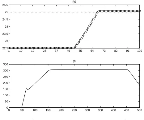
7(t) and desired traffic density trajectory ρ5d7(t) in Figure 1 (d) fort∈ {0,1,2,· · ·,500}. To see the control behavior thatρ5₇(t)is close toρ5_d7(t)fort∈ {0,1,2,· · ·,500} except the initial fifty discrete-time, the trajectories between ρ5₇(t) and ρ5

d7(t) are shown again in Figure 1 (e) only for the time sequence t ∈ {0,1,2,· · ·,100}. It is clear that ρ5

7(t) converges toρ5

d7(t)after t≥50. Finally, Figure 1(f) shows the bounded learned control input r5

7(t) for the 7th traffic flow subsystem.

VI. CONCLUSION

1 10 19 28 37 46 55 64 73 82 91 100 22.5

23 23.5 24 24.5 25 25.5

(e)

0 50 100 150 200 250 300 350 400 450 500

0 50 100 150 200 250 300 350

[image:6.595.53.286.55.250.2]

(f)

Fig. 1. (a) sj₄(t) versus time t; (b)maxt∈{1,···,500}|ejφ7(t)|

ver-sus control iteration j; (c)e5

7(t) (solid line) and θ57(t)

¡¯_¯ Θ5

7(t)

¯ ¯ ₊ 1¢,−θ5

7(t)

¡¯_¯ Θ5

7(t)

¯

¯_{+ 1}¢_{(dotted lines) versus timet∈ {1,2,· · ·,500};} (d)ρ5

7(t) (solid line) and ρ

j

d7(t) (dotted line) versus time t ∈

{0,1,· · ·,500} at the 5th control iteration; (e)ρ5

7(t)(◦ ◦ ◦) andρ5d7(t)

(· · ·) versus timet∈ {0,1,· · ·,100}at the 5th control iteration; (f)r5 7(t)

versus timet.

For further compensation of the lumped uncertainties in-duced by function approximation errors and random off-ramp traffic volumes of the freeway, a dead-zone like auxiliary traffic density error functions with time-varying boundaries are then constructed. By the auxiliary traffic density error functions, the adaptive laws for the control parameters and time-varying boundary layer are designed to guarantee the closed-loop stability and learning error convergence. Based on a Lyapunov like analysis, we show that all adjustable parameters and the internal signals remain bounded and the traffic density tracking errors asymptotically converge to a residual set whose size depends on the width of boundary layer as iteration goes to infinity.

ACKNOWLEDGMENT

This work is supported by Ministry of Science and Tech-nology, Taiwan, under Grants MOST104-2221-E-211-009 and MOST104-2221-E-211-010.

REFERENCES

[1] M. Papageorgiou and A. Kotsialos, “ Freeway ramp metering: an overview,” IEEE Transactions on Intelligent Transportation Systems, Vol. 3, No. 4, pp. 271 281, 2002.

[2] M. Papageorgiou, H. Hadj-Salem , J. M. Blosseville, “ALINEA: A local feedback control law for on-ramp metering,” Transportation Research

Record, No. 1320, pp. 58 64, 1991.

[3] H.M. Zhang, S.G. Ritchie, R. Jayakrishnan, “ Coordinated traffic-responsive ramp control via nonlinear state feedback,” Transportation

Research Part C, Vol. 9, No. 5, pp. 337 352, 2001.

[4] A. Kotsialos, “Coordinated and integrated control of motor-way net-works via nonlinear optimal control,” Transportation Research Part C, Vol. 10, No. 1, pp. 65 84, 2002.

[5] Z. S. Hou, J. X. Xu and H. W. Zhong, “Freeway trame control using iterative learning control based ramp metering and speed signaling,”

IEEE Transactions on Vehicular Technology, Vol. 56, Issue: 2, pp. 466

477, 2007.

[6] Z. S. Hou, J. X. Xu, and J. W. Yan, ‘An iterative learning approach for density control of freeway traffic flow via ramp metering,” Transp.

Res., Part C, Vol. 16, No. 1, pp. 71 97, 2008.

[7] Z. S. Hou, J. W. Yan, J.-X. Xu and Z. J. li, “Modified iterative-learning-control-based ramp metering strategies for freeway traffic control with iteration-dependent factors,” IEEE Transactions on Intelligent

Trans-portation Systems, Vol. 13, Issue: 2, pp. 606 618, 2012.

[8] M. Papageorgiou, J. M. Blosseville and H. Hadj-Salem, “Macroscopic modeling of traffic flow on the Boulevard Peripherique in Paris,”

Transportation Research Part B, Vol.23 No. 1, pp. 29 47, 1989. [9] Y.C. Wang and C.J. Chien, “Repetitive tracking control of nonlinear

systems using reinforcement fuzzy-neural adaptive iterative learning controller,” Applied Mathematics and Information Sciences, vol. 6, no. 3, pp. 473-481, 2012.

[10] Y.C. Wang and C.J. Chien, “Design and analysis of fuzzy-neural discrete adaptive iterative learning control for nonlinear plant,”