Testing the Adding up Condition in Demand Systems

http://www.scirp.org/journal/ojs ISSN Online: 2161-7198

ISSN Print: 2161-718X

DOI: 10.4236/ojs.2017.72022 April 26, 2017

Testing the Adding up Condition in Demand

Systems

Quirino Paris

1

, Francesco Caracciolo

2

1_{Department of Agricultural and Resource Economics, University of California, Davis, USA}

2_{Department of Agricultural Sciences, University of Naples, Federico II, Portici, Italy}

Abstract

A test of the adding up condition in demand systems is crucial for determin-ing whether a share format is admissible when the number of sample goods is smaller than the number of commodity choices available to consumers. This test requires the estimation of a demand system in a quantity format. It can-not be performed when a demand system is specified in share format. The share specification of any demand system is like a straight jacket: once worn, it forces the error covariance matrix to be singular and the adding up condi-tion to hold whether or not the data generating process warrants it. The em-pirical verification of the adding up hypothesis uses a five-commodity sample selected from the Canadian Family Expenditure Survey with 4847 observa-tions. Three specifications are considered: AIDS (Almost Ideal Demand Sys-tem), QUAIDS (Quadratic AIDS) and EASI (Exact Affine Stone Index). The hypothesis is rejected in all three cases with a high level of confidence.

Keywords

Adding up, Demand Systems, Quantity Format, Share Format

1. Introduction

The objective of this paper is to discuss the importance of testing the adding up condition in a demand system as a gateway to the estimation of the correspond-ing expenditure-share specification.

To summarize the discussion elaborated further on, the advantages of a share format may be listed as saving degrees of freedom and mitigating error hete-roskedasticity. The limitations are, perhaps, more eye opening. A crucial issue consists in the impossibility of testing a null hypothesis such as the adding up condition that is automatically satisfied in an expenditure-share format and in-duces the singularity of the error covariance matrix. In a share format, adding up, How to cite this paper: Paris, Q. and

Ca-racciolo, F. (2017) Testing the Adding up Condition in Demand Systems. Open Jour- nal of Statistics, 7, 290-304.

https://doi.org/10.4236/ojs.2017.72022

Received: February 16, 2017 Accepted: April 23, 2017 Published: April 26, 2017

Copyright © 2017 by authors and Scientific Research Publishing Inc. This work is licensed under the Creative Commons Attribution International License (CC BY 4.0).

http://creativecommons.org/licenses/by/4.0/

symmetry and homogeneity are hypotheses that cannot be tested independently. Testing the adding up condition is important because, often, the number of sam-ple commodities is much smaller than the number of goods that compose a consumer’s basket. This hypothesis and the associated statistical test constitute the paper’s main focus.

The advantages of a quantity format can be listed as the possibility of testing the adding up condition, the zero-degree homogeneity assumption and the sym- metry and negative semidefiniteness of the Slutsky matrix as separate null hy-potheses. The disadvantages are minimal and deal, possibly, with the necessity of requiring larger samples than in the case of a share format. This event may occur in very small samples.

Given the gamut of issues associated with the estimation and testing of con-sumer demand systems, we will narrow this preliminary discussion to specifica-tions of share systems as commonly appeared in the literature. The pioneering paper by Sir Richard Stone [1], presents a linear expenditure system (LES) of demand functions stated in expenditure format, where the dependent variable represents the expenditure on a given good. This specification is equivalent to a share format where the share is defined with respect to total expenditure. Stone’s LES empirical model includes all goods and services grouped in six categories of commodities for the years 1920 to 1938 in the United Kingdom. For the first time, the theoretical requirements of adding up, zero-degree homogeneity of demand functions and symmetry of the Slutsky matrix appear as restrictions in the empirical literature. Barten [2], who presented a linear demand system that is stated directly in share format, attempted to include all commodities in the consumer expenditure household survey kept in The Netherlands between 1921 and 1958. There followed other important papers by Barten [3], in share format and by Pollak and Wales [4], in expenditure format. Hence, the tradition of es-timating demand systems in expenditure-share format has a distinguished li-neage.

In his influential paper that summarizes the empirical literature on consumer demand, Barten ([5], p. 23) wrote: “The approach is essentially an empirical one, in the sense that one aims at the formulation of a system to be estimated using actual data. In view of the data limitations, one makes use of restrictions which, in part, are of a theoretical nature.” We interpret Barten’s words to mean that the data generating process (DGP) ought to assume center stage in an econome-tric specification of models that wishes to represent the final decisions of con-sumer behavior. In econometrics, a DGP must be guided by economic theory but must also be adapted to describe the peculiarities of data collection, as Bar-ten implicitly suggests.

In the case of consumer behavior, utility theory develops the process of deriv-ing systems of demand functions in the format of quantity levels of various commodities as a function of their prices and income. Let

q

be an

N

-vector

of quantity levels of

N

commodities and services that represent all the goods’

292

goods. Finally, let m be the exogenous income available to consumer for mak-ing her

N

decisions. Then, utility theory derives a system of

(

N+1

)

relations

that are interpreted as

N

Marshallian demand functions and a budget

con-straint

(

,

)

q=q p m (1)

q p′ =m. (2)

The

(

N+1

)

system has

N

unknown quantities,

q

, and, therefore, one of

the

N

relations in Equation (1) is redundant and can be omitted in the

solu-tion of the remaining

(

N−1

)

quantities. The quantity of the

N

-th good can

be recovered from the budget constraint after replacing the

(

N−1

)

quantities

obtained from the solution of the

(

N−1

)

relations.

In many cases, however, the DGP of consumer demand information, in any given sample, may not satisfy all the conditions stated above. Many empirical studies that estimate systems of demand functions exhibit a number of com-modities,

n

<

N

, that is much smaller than the number of all possible goods

available for consumers’ decisions over a given time interval. In this case, the sample demand system is incomplete [6]. It does not satisfy the adding up con-dition since m represents exogenous income that is available for purchasing all the commodities of consumers’ choice.

It is well known that the hypotheses of separability and multistage budgeting were developed to justify the adoption of the features associated with the general theoretical scaffolding also in the case of a small number of commodities (or commodity aggregates). Accordingly, consumption decisions would occur in at least two stages. In the first stage, consumer would allocate income among a number of commodity subsets. In the second stage, consumer would proceed to maximize utility only with respect to the commodities belonging to one of those subsets subject to the previously determined portion of income for that category of goods. All this development is acceptable from a theoretical standpoint. In an empirical setting, however, these hypotheses remain often untested and untesta-ble, given the available sample information. Put another way, the portion of in-come that, according to a two-stage approach of consumer decisions, would be allocated to a specific commodity subset in the first stage is never known and measurable, thus preventing the testing of the assumption that would require this level of income to be an exogenous piece of information. We emphasize, therefore, that to test the hypothesis whether a group of

n

<

N

commodities is

separable from the rest of the consumer’s basket it is necessary to collect sample information on quantities and prices on all the

N

goods.

Equ-ation (1) while the analogous EquEqu-ation (2) is not a constraint but is simply an accounting relation with no sample information of its own that is independent of prices and quantities. Many empirical studies of demand published to date, however, have taken for valid both Equations (1) and (2), regardless of the subset of commodities dealt with in the sample and without performing a statistical test of the adding up condition. This test appears to represent a crucial step for as-sessing the theoretical scaffolding leading to a share format: If constraint (2) is part of the hypothesis that the sample commodities constitutes a proper subset of goods within a two-stage budgeting process, the test of the adding up condi-tion is an indicator of whether that hypothesis may be supported by the sample data.

Referring to a stochastic specification of a demand system described by the theoretical scaffolding of Equations (1) and (2), the fundamental, empirical sequence of the assumptions and conclusions that are valid for the entire con-sumer’s basket is stated by Barten ([5], p. 26) as: “However, Equation (2) implies a linear dependence of the joint distribution of the disturbances if m and p are exogenous. The theoretical covariance matrix is, therefore, singular. This prob-lem is usually solved by deleting one equation from the system.”

This proposition was originally put forward in the late sixties, [7], and, since then, almost all the empirical studies of demand that appeared in the literature have adopted it regardless of the number of commodities involved and whether the available information constitutes an incomplete sample. Furthermore, the great majority of studies has gone another step and has specified demand sys-tems in the format of expenditure shares. Deaton and Muellbauer [8], with their Almost Ideal Demand System (AIDS), have provided a remarkable impetus for the use of an expenditure-share format in empirical studies of demand.

Thus, in this cursory survey of empirical demand issues, we have identified two main topics of interest. The first topic deals with the question whether the DGP of sample information of consumer behavior-as typically observed-statis- tically supports the application of the more general approach embedded in Equ-ations (1) and (2), regardless of the size and completeness of the subset of com-modities constituting the sample data. The second topic discusses the conse-quences of estimating demand systems in expenditure-share format rather than in a quantity format. In particular, given the absence of empirical information about a two-stage budgeting and separability that characterizes many empirical demand studies, it is of interest to know whether the adding up condition holds for the sample at hand. As elaborated in more detail further on, this condition is crucial for concluding that the error covariance matrix is singular and, as a con-sequence, for admitting the deletion of an equation in the estimation of demand parameters without loss of information. The adding up condition, however, cannot be tested using an expenditure-share format of the demand system. This test must be performed using a quantity format.

294

share format. Section 3 lays out the stochastic quantity model of demand func-tions based upon the AIDS specification of Deaton and Muellbauer [8], as the most popular demand system appeared so far in the literature. Two more recent specifications will also be presented: the quadratic AIDS (QUAIDS) of Banks, Blundell and Lewbel [9], and the EASI (Exact Affine Stone Index) demand sys-tem of Lewbel and Pendakur [10]. Section 4 describes a large sample of data used in the empirical analysis and presents the empirical results. Conclusions follow.

2. Models in Share Format

Any linear statistical model that is specified in share format, with an intercept in each equation and the same explanatory variables appearing in every equation, exhibits a unique property: the sum over equations of the error terms is equal to zero in each sample observation. Therefore, the error covariance matrix is sin-gular. Furthermore, the sum over intercepts of the various equations is equal to 1 and the sum over rows of the coefficient matrix associated with explanatory va-riables is equal to zero without any a priori condition on parameters. Hence, the adding up property of shares holds automatically on the left and on the right side of the equality sign. This result is briefly mentioned in papers by Worswick and Champernowne [11], Barten [7], Berndt and Savin [12]. We offer an alter-native derivation in the Appendix. Surprisingly, however, many demand studies that specify a share format declare that the adding up restrictions must be im-posed on the model’s parameters. For example, Berndt and Savin ([12], p. 938) write: “It is assumed that y satisfies the adding up conditions …”; Moschini ([13], p. 351) writes: “… adding up … hold(s) if …”; Alston, Chalfant and Piggott ([14], p. 74) write: “To satisfy … adding up … the following restrictions must hold …”; Fisher, Fleissig and Serletis ([15], p. 62) write: “Adding up … restric-tions require that …”; Cranfield, Eales, Hertel and Preckel ([16], p. 357) write: “Adding up is imposed with …”; Barnett and Serletis ([17], p. 213) write: “… the resulting theoretical restrictions are …”; Liu, Parton, Zhou and Cox ([18], p. 488) write “… to be consistent with the demand theory, the following restrictions must be adhered to: the adding up restriction …”. This oversight may have con-sequences for testing hypotheses.

Let t=1,,T indicate sample observations; k=1,,K the number of

equations; j=1,,J the number of explanatory variables; wkt the share of the k−th equation in the t−th observation; pjt the j−th explanatory variable in the t−th observation; bk the intercept in the k−th equation;

jk

a the j−th parameter in the k−th equation; ukt the disturbance term of the k−th equation in the t−th observation with expectation E u

( )

kt =0

and constant

(

K×K

)

contemporaneous covariance matrix Σ_u. All

explana-tory variables appear in each equation. Then, a share model without theory is stated as

1

.

J

kt k jk jt kt j

w b a p u

=

Summing over equations

1 1 1 1 1

1

K K K J K

kt k jk jt kt

k k k j k

w b a p u

= = = = =

=

∑

=

∑

+

∑∑

+

∑

_{. (4)}

In the Appendix, it is shown that the sum over equations of relation (3) fulfills the adding up property automatically without imposing any a priori additional constraints on the parameters of the share-model specification of Equation (3). In other words,

1 1 1 1 1

1; 1; 0; 0

K K K J K

kt k jk jt kt

k k k j k

w b a p u

= = = = =

= = = =

∑

∑

∑∑

∑

. (5)

The contemporaneous error terms ukt form a linear combination in each observation and the estimated error covariance matrix is singular. Therefore, any estimator that requires the inversion of the error covariance matrix Σu is infeasible. Notice that

1 1

1 and 0, 1, ,

K K

k jk

k k

b a j J

= =

= = =

∑

∑

 (6)

without the necessity to impose these conditions as a priori restrictions. Hence, an equation can be deleted from system (3) and the estimates of the corres-ponding parameters can be recovered from relations (6).

The relationship between this discussion of a general share system such as Equation (3) and an expenditure-share system of demand functions, as usually stated in the literature, is straightforward. Many demand studies appeared in print and specified in expenditure-share format-although they deal with a num-ber of commodities

n

<

N

-have all explicitly assumed and imposed adding up

conditions by way of parameter restrictions analogous to relations (6). But since the adding up condition holds by necessity without the need to impose it a priori, this suggests that the share specification of any econometric model (and, equi-valently, the expenditure specification of it) is like a straight jacket: once worn, it forces the error covariance matrix to be singular and the adding up condition to hold whether or not the DGP warrants it. An important corollary follows: the null hypothesis that the adding up condition holds cannot be tested under a share (expenditure) format of demand systems. In the absence of any sample in-formation regarding a two-stage budgeting, the test of the null hypothesis that the adding up condition holds corresponds to an indirect test of the assumption that the sample commodities constitutes a proper subset of goods in a two-stage budgeting process of consumer behavior. To test this null hypothesis, however, only a quantity format specification of a demand system is available.

To exemplify more directly that the above reasoning applies also to demand systems, we state the AIDS model of Deaton and Muellbauer [8], in share format

1

log log

n

t

kt k ki it k kt

i t

x

w p u

P

α γ β

=

  = + + _{ }+

 

∑

(7)

where k=1,, ; n i=1,,n and t=1,,T . All logarithms in this paper are

296

senting quantities and prices of the t−th sample observation while total

ex-penditure is 1 n t k kt kt

x =

∑

₌ q p with shares computed as w_kt =q p_{kt kt} x_t . Further-

more, the deflating price index is defined as

( ) ( )

0

1 1 1

1

log log log log

2

n n n

t i it ik it kt

i i k

P α α p γ p p

= = =

= +

∑

+

∑∑

₍₈₎

although Deaton and Muellbauer suggested and many empirical studies adopted their suggestion that a Stone index could often suffice:

1 log

n t it it

i

P∗ w p

=

=

∑

_{. (9)}

Furthermore, Deaton and Muellbauer specify and impose parameter restric-tions that include adding up requirements, zero-degree homogeneity in prices and income of demand functions and symmetry of the Slutsky matrix

1 1 1

1, 0, 0

n n n

k ki k

k k k

α γ β

= = =

= = =

∑

∑

∑

adding up (10)

1 0

n ki i

γ

=

=

∑

zero-degree homogeneity (11)

ki ik

γ =γ _{Slutsky symmetry (12)} and write ([8], p. 314): “Provided (10), (11), and (12) hold, Equation (7) re- presents a system of demand functions which add up to total expenditure, are homogeneous of degree zero in prices and total expenditure taken together, and which satisfy Slutsky symmetry.” But, as argued above, restrictions (10) are au-tomatically satisfied in a share system regardless of either theory or other as-sumptions. They are satisfied automatically also when conditions (11) and (12) are imposed using either specification of the price index deflator. Hence, there is no need to state them as if they “ought to be imposed” for estimating a share model which represents a demand system.

Thus, the estimation of Equations (7) and (8) [or (9)] together with side con-ditions (11) and (12) represents a special case of estimating the share system (3). Barten ([7], p. 16) stated: “… it is possible to delete one equation from the sys-tem without losing any information.”1 _{After the knowledge acquired from the} above discussion, this statement should be qualified to read: “When a share for-mat is warranted, it is possible to delete one equation from the system without losing any information.”

With respect to parameter “restrictions” (10) a crucial remark is in order. They imply that the general theoretical conclusions of consumer theory, which are valid for the full basket of

N

commodities, have been adopted also for the

case when the number of sample goods is

n

<

N

. Furthermore, the adding up

hypothesis cannot be tested in an expenditure-share demand system. Hence, suppose that the adding up condition does not hold (tested in a quantity format model). This means that the number of sample commodities is different from

1_{But Barten also wrote ([7], p. 16): “However, it is quite arbitrary as to which equation should be}

the number of goods constituting a proper subset, according to a two-stage budgeting criterion.

3. AIDS, QUAIDS and EASI Quantity Formats

Under the assumptions of an AIDS expenditure function, consumer utility theory generates a system of demand functions that assumes the following quan-tity format in a stochastic representation

(

)

1

log log ,

n

t t t t

it i ij jt i it i t it

j

it it t it

x x x x

q p v g x p

p p P p

α γ β

=

 

= + + _{ } +

 

∑

(13)

where i j, =1,,n and vit is a disturbance term for the i th− commodity in the t−th _{observation with expectation} E v

( )

it =0 and covariance matrix Σv. According to Brown and Walker, [19], the disturbance terms of commodities involved in the individual consumer’s decisions may depend on prices and total expenditure. To represent this assumption about heteroskedasticity the function

(

,

)

i t it

g x p multiplies the disturbance term with the objective of rendering the

entire error term homoskedastic.

Model (13) can now be used to test a series of null hypotheses based upon re-strictions (10), (11) and (12). The tests have the structure of a likelihood ratio which is distributed as a chi square with degrees of freedom equal to the number of restrictions. In particular, we are interested in testing the adding up hypothe-sis expressed by restrictions (10).

The QUAIDS specification in quantity format takes on the following expres-sion (see [9], p. 534):

( )

( )

( )

(

)

1 2 log log log , n

t t t t

it i ij jt i

j

it it it

i t t

it i t it it

x x x x

q p

p p a P p

x x

v g x p

b P a P p

α γ β

λ =   = + +          +    +     

∑

(14) where

( )

0

( ) ( )

1 1 1

1

log log log

2

n n n

i it ik it kt

i i k

a P α α p γ p p

= = =

= +

∑

+

∑∑

_,

( )

n₁ i

it i

b P =

∏

₌ pβ .

In this case, the adding up hypothesis requires the same AIDS relations (10) with the addition that

1 0 n i i λ = =

∑

. (15)

298

for clarity, the range of the various indexes: observations are denoted by

1, ,

t= T ; equations by i k, =1,,n; demographic variables by l=0,1,,L;

0t 1 for all

z = t; the power of log expenditure by r=0,1,,R. The EASI

de-mand system, then, takes on the following specification in quantity format

( )

( )

0 0 0

1 0 1

log log

R L L

r t t t

it ir t il lt il lt t

r it l it l it

n L n

t t

ikl lt kt ik t it it

k l it k it

y y y

q b y C z D z y

p p p

y y

A z p B y p

p p ε

= = =

= = =

= + +

+ + +

∑

∑

∑

∑∑

∑

(16)

where

( ) ( )

( ) ( )

1 0 1 1

1 1

log log log log 2

.

1 log log 2

n L n n

t k kt kt l lt i k ikl it kt

t n n

ik it kt i k

x w p z A p p

y

B p p

= = = = = = − + = −

∑

∑

∑ ∑

∑ ∑

(17)

The variable yt is the logarithm of real expenditure defined as nominal log expenditure, logxt, deflated by the Stone index and other price terms. The in-troduction of two-way interactions of the demographic variables with prices and total expenditure follows the specification of Lewbel and Pendakur [10].

The adding up constraint of the EASI model is satisfied with the following parametric conditions

0

1 1 1 1

1 1

1, 0, for 0, 0

0 0,1, , , 1, , .

n n n n

i ir il il

i i i i

n n

ikl ik

i i

b b r C D

A B l L k n

= = = = = = = = ≠ = = = = = =

∑

∑

∑

∑

∑

∑

  (18)

The flexibility of the EASI demand system is reflected in the number of para-meters to be estimated. For example, with 5 commodities, 5 demographic variables and the exponent of the logarithm of real expenditure equal to 5, the number of parameters to be estimated is 255. A sample of 4847 observations was used.

The rejection of the null hypothesis that the adding up restrictions hold would implies that an expenditure-share format of the demand system is unwarranted. In that case, the use of a share format of the demand system and the drop of an equation for its estimation would correspond to a loss of information because the error covariance matrix of the quantity model is not singular.

4. Data and Results

trans-fers are greater than 10 percent of gross income; and 5) a time variable equal to the calendar year minus 1986 (that is, equal to zero in 1986). These demographic variables are indicated as Z variables. For a more detailed description of the sample data see Lewbel and Pendakur ([10], pp. 839-840).

We reiterate that the principal objective of this paper consists in testing the adding up hypothesis in the estimation of demand systems with an incomplete sample of consumer data because this event is the prevalent occurrence in the empirical literature. Again, an incomplete sample occurs when the commodity categories employed in the empirical estimation do not exhaust the commodities available to consumers’ choice. In the case of the Lewbel and Pendakur database, the presumption is that the 9 categories of goods do, indeed, form a complete sample. Therefore, in order to conform to the context of this paper, the follow-ing 5 categories were selected: food-in, rent, clothfollow-ing, transportation operation and recreation.

For the empirical context described above, the crucial test deals with the add-ing up hypothesis that, as elaborated in previous sections, cannot be performed using an expenditure-share format of a demand system. Thus, it is the main contention of this paper that a share specification will not imply a loss of infor-mation only when the adding up hypothesis will not be refuted by an appropri-ate statistical test.

For the AIDS model, this hypothesis requires testing the restrictions of Equa-tion (10). For the QUAIDS model, the restricEqua-tions are stated in EquaEqua-tions (10) and (15). For the EASI model, the restrictions to test are specified in Equation (18). In all three cases, the parameters of the demographic Z variables require a zero sum over equations.

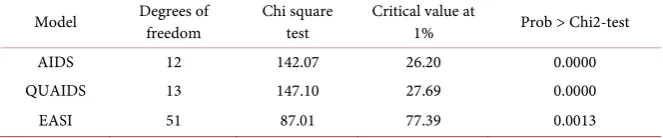
In all three specifications, the null hypothesis is rejected at a very high confi-dence level (see Table 1). It is important to remark that in all these 5-commodity systems of equations, the estimated error covariance matrix is not singular and, indeed, it is associated with a condition number of about 15.0, well below the empirical cut off point of 30.0 suggested by Besley, Kuh and Welsch [21], as an indication of collinearity. This means that the estimated errors of the 5-com- modity model are not linearly dependent and dropping one equation, as the es-timation of a share model requires, amounts to forcing the original quantity model into a straight jacket resulting in a loss of information.

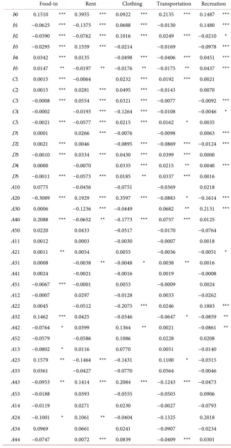
[image:10.595.207.539.661.730.2]

The estimated parameters of the EASI model are reported in Table 2 for the unrestricted version of the demand system. Given the large number of estimated parameters (255) the relevant statistics are given in condensed form. One, two

Table 1. Test results of the adding up hypothesis.

Model Degrees of _freedom Chi square _test Critical value at _1% Prob > Chi2-test

AIDS 12 142.07 26.20 0.0000

QUAIDS 13 147.10 27.69 0.0000

[image:11.595.202.536.92.739.2]

300

Table 2. FIML estimates of the EASI model.

Food-in Rent Clothing Transportation Recreation

b0 0.1510 *** 0.3955 *** 0.0922 *** 0.2135 *** 0.1487 ***

b1 −0.0625 *** −0.1375 *** 0.0688 *** −0.0130 0.1480 ***

b2 −0.0390 *** −0.0762 *** 0.1016 *** 0.0249 *** −0.0210 *

b3 −0.0295 *** 0.1559 *** −0.0214 −0.0169 −0.0978 ***

b4 0.0342 *** 0.0135 −0.0498 *** −0.0406 *** 0.0451 ***

b5 0.0147 ** −0.0197 ** −0.0176 ** −0.0175 ** 0.0437 ***

C1 0.0015 *** −0.0064 0.0232 *** 0.0192 *** 0.0021

C2 0.0015 *** 0.0281 *** 0.0495 *** −0.0143 0.0070

C3 −0.0008 *** 0.0554 *** 0.0321 *** −0.0077 −0.0092 ***

C4 −0.0002 −0.0193 *** −0.1264 *** −0.0108 −0.0046 *

C5 −0.0021 *** −0.0577 *** 0.0215 *** 0.0162 * 0.0035

D1 0.0001 0.0266 *** −0.0076 −0.0098 0.0063 ***

D2 0.0021 *** 0.0046 −0.0895 *** −0.0869 *** −0.0124 ***

D3 −0.0010 *** 0.0334 *** 0.0430 *** 0.0399 *** 0.0000

D4 0.0000 −0.0070 0.0335 *** 0.0215 ** 0.0040 ***

D5 −0.0011 *** −0.0573 *** 0.0185 ** 0.0337 *** 0.0016

A10 0.0775 −0.0456 −0.0751 −0.0369 0.0218

A20 −0.3089 *** 0.1929 *** 0.3597 *** −0.0883 * −0.1614 ***

A30 0.0006 −0.1236 *** −0.0449 0.0682 ** 0.2131 ***

A40 0.2088 *** −0.0652 ** −0.1773 *** 0.0757 *** 0.0125

A50 0.0220 0.0433 −0.0517 −0.0170 −0.0764

A11 0.0012 0.0003 −0.0030 −0.0007 0.0018

A21 0.0011 ** 0.0054 0.0055 −0.0036 −0.0051 *

A31 0.0008 −0.0038 ** −0.0048 * 0.0038 ** 0.0016

A41 0.0024 −0.0021 −0.0016 0.0019 −0.0008

A51 −0.0067 *** −0.0001 0.0053 −0.0009 0.0024

A12 −0.0007 0.0297 −0.0128 0.0033 −0.0262

A22 0.0045 −0.0512 −0.2075 *** 0.0246 0.1883 ***

A32 0.1462 *** 0.0425 −0.0346 −0.0647 * −0.0859 **

A42 −0.0764 * 0.0399 0.1364 ** 0.0021 −0.0861 **

A52 −0.0579 −0.0586 0.1086 0.0228 0.0208

A13 −0.0802 * 0.0116 0.0770 0.0051 −0.0140

A23 0.1579 ** −0.1464 *** −0.1431 0.1100 * −0.0315

A33 0.0361 −0.0427 −0.0770 0.0564 −0.0046

A43 −0.0953 ** 0.1414 *** 0.2084 *** −0.1243 *** −0.0473

A53 −0.0188 0.0393 −0.0555 −0.0503 0.0906

A14 −0.0119 0.0271 0.0230 −0.0027 −0.0793

A24 −0.1001 * 0.1061 ** −0.0404 −0.1325 0.2018

A34 0.0969 0.0661 0.0241 −0.0907 −0.0234

Continued

A54 0.1163 −0.2097 −0.1540 0.2606 −0.0890

A15 0.0029 −0.0079 *** −0.0041 0.0088 ** −0.0043

A25 0.0019 0.0047 −0.0243 ** 0.0035 0.0029

A35 −0.0129 *** 0.0001 *** 0.0313 0.0050 −0.0157 ***

A45 −0.0025 0.0073 *** 0.0155 ** −0.0093 *** 0.0004

A55 0.0083 −0.0072 * −0.0145 −0.0044 0.0146 ***

B1 0.0739 0.1742 *** −0.1213 −0.0955 * −0.1656 ***

B2 −0.6354 *** 0.0710 0.3880 *** 0.0417 0.4151 ***

B3 0.1364 ** −0.1167 ** −0.0102 0.0847 −0.0970

B4 0.1277 ** 0.0362 0.0029 0.0156 *** −0.2610 ***

B5 0.2631 *** −0.1754 *** −0.2262 * −0.0407 0.1223

*, **, *** correspond to 0.1, 0.05, 0.01 confidence levels, respectively.

and three asterisks correspond to a confidence level threshold of 0.10, 0.05 and 0.01, respectively.

The parameter estimates of bir, 1,r= , 5 are highly significant and attest to

the complex shape of the Engel curves for each of the five commodity categories. The price-slope coefficients, Aik l,=0, are also highly significant. The parameters of the demographic variables and their interactions with total expenditure and prices make up the large body of estimates and suggest the plausibility of the two-way specification of interaction effects.

5. Conclusions

This paper’s motivation springs from the question of whether a share format of demand systems is warranted even in cases when the data sample deals with a rather small number of consumer goods. That is, when the sample is incomplete in the sense that the number of consumer goods is smaller (sometimes much smaller) than the number of commodity choices available to consumers. The adding up condition was identified as a crucial restriction that may not be at-tained when demand systems are incomplete. In such cases, the error covariance matrix of the empirical model (specified in quantity format) is not singular and a share format is unwarranted because dropping one equation—as customarily done in the estimation of share specifications—corresponds to losing sample in-formation.

The estimation of a quantity format does not involve any additional difficul-ties over those ones encountered in the estimation of share formats. Quantity formats, furthermore, allow for testing of all the relevant hypotheses of consum-er theory, including the adding up restrictions—an hypothesis that is precluded by share formats.

re-302

jected with a high degree of confidence in all the three specifications of the de-mand system.

References

[1] Stone, R. (1954) Linear Expenditure Systems and Demand Analysis: An Application

to the Pattern of British Demand. The Economic Journal, 64, 511-527.

https://doi.org/10.2307/2227743

[2] Barten, A.P. (1964) Consumer Demand Functions under Conditions of Almost

Ad-ditive Preferences. Econometrica, 32, 1-38.

[3] Barten, A.P. (1968) Estimating Demand Functions. Econometrica, 36, 213-251.

[4] Pollak, R.A. and Wales, T.J. (1969) Estimation of the Linear Expenditure System.

Econometrica, 37, 611-628.

[5] Barten, A.P. (1977) The System of Consumer Demand Functions Approach: A

Re-view. Econometrica, 45, 23-50.

[6] LaFrance, J.T. and Hanemann, W.M. (1989) The Dual Structure of Incomplete

De-mand Systems. American Journal of Agricultural Economics, 71, 262-274.

https://doi.org/10.2307/1241583

[7] Barten, A.P. (1969) Maximum Likelihood Estimation of a Complete System of

De-mand Equations. European Economic Review, 1, 7-73.

[8] Deaton, A. and Muellbauer, J. (1980) An Almost Ideal Demand System. American

Economic Review, 70, 312-326.

[9] Banks, J., Blundell, R. and Lewbel, A. (1997) Quadratic Engel Curves and Consumer

Demand. Review of Economics and Statistics, 79, 527-539.

https://doi.org/10.1162/003465397557015

[10] Lewbel, A. and Pendakur, K. (2009) Tricks and Hicks: The EASI Demand System.

American Economic Review, 99, 827-863. https://doi.org/10.1257/aer.99.3.827

[11] Worswick, G.D.N. and Champernowne, D.G. (1954-1955) A Note on the

Add-ing-Up Criterion. The Review of Economic Studies, 22, 57-59.

https://doi.org/10.2307/2296224

[12] Berndt, E.R. and Savin, N.E. (1975) Estimation and Hypothesis Testing in Singular

Equation Systems with Autoregressive Disturbances. Econometrica, 43, 937-958.

[13] Moschini, G. (1998) The Semiflexible Almost Ideal Demand System. European

Economic Review, 42, 349-364.

[14] Alston, J.M., Chalfant, J.A. and Piggott, N.E. (2001) Incorporating Demand Shifters

in the Almost Ideal Demand System. Economics Letters, 70, 73-78.

[15] Fisher, D., Fleissig, A.R. and Serletis, A. (2001) An Empirical Comparison of

Flexi-ble Demand System Functional Forms. Journal of Applied Econometrics, 16, 59-80.

https://doi.org/10.1002/jae.585

[16] Cranfield, J.A.L., Eales, J.S., Hertel, T.W. and Preckel, P.V. (2003) Model Selection

When Estimating and Predicting Consumer Demands Using International, Cross

Section Data. Empirical Economics, 28, 353-364.

https://doi.org/10.1007/s001810200135

[17] Barnett, W.A. and Serletis, A. (2008) Consumer Preferences and Demand Systems.

Journal of Econometrics, 147, 210-224.

[18] Liu, H., Parton, K.A., Zhou, Z.Y. and Cox, R. (2009) At-Home Meat Consumption

in China: An Empirical Study. Australian Journal of Agricultural and Resource

[19] Brown, B.W. and Walker, M.B. (1989) The Random Utility Hypothesis and

Infe-rence in Demand Systems. Econometrica, 57, 815-829.

[20] Gorman, W.M. (1981) Some Engel Curves. In: Deaton, A., Ed., Essays in the Theory

and Measurement of Consumer Behaviour: In Honour of Sir Richard Stone, Cam-bridge University Press, CamCam-bridge, 7-30.

https://doi.org/10.1017/cbo9780511984082.003

[21] Besley, D.A., Kuh, E. and Welsch, R.E. (1980) Regression Diagnostics. Identifying

Influential Data and Sources of Collinearity. Wiley Interscience, New York.

304

Appendix

The sum over equations of the intercepts in any seemingly unrelated equation system specified in share format (with the same explanatory variables entering every equation) is equal to one. The sum over equations of the slope coefficients is equal to zero. As a consequence, the sum over equations of the disturbance terms is equal to zero and the associated error covariance matrix is singular.

In order to simplify the notation the observation index is omitted. Let 1, ,

k=  K be the number of equations in share format. The number of shares is divided into a vectorwK′ =−1

[

w1,,wK−1

]

of the first

(

K−1

)

shares and the last k−th share wK. Disturbance terms are divided into a vector

[

]

1 1, , 1

K− u uK− ′ =

u  of the first

(

K−1

)

terms and the last u_K item. The

num-ber of intercepts is divided into a vector bK′ =−1

[

b1,,bK−1

]

of the first

(

K−1

)

intercepts and the last of them, bK. Let p′ =

[

p1,,pJ

]

be a vector of

J

ex-planatory variables that enter each share equation. The j−th column of the

matrix of unknown slope parameters is divided into a vector aK−1,j and the last slope parameter aK j, . The vector sK′ =−1

[

1,,1

]

is a

(

K−1

)

sum vector of unitary coefficients.

The K-equation system in share format can now be stated as

1 1 1, 1

1

J

K K K j j K

j

p

− − − −

=

= +

∑

+

w b a u (A.1)

, 1

J

K K K j j K j

w b a p u

=

= +

∑

+ _{. (A.2)}

The pre-multiplication of system (A.1) by the sum vector sK′−1 results in

1 1 1 1 1 1, 1 1

1

J

K K K K K K j j K K j

p

− − − − − − − −

=

′ = ′ +

∑

′ + ′

s w s b s a s u . (A.3)

Given the share format, Equation (A.2) can be restated as

1 1 ,

1 1

J

K K K K K j j K j

w _{− −} b a p u

= ′

= −s w = +

∑

+ (A.4)

and rearranging Equation (A.4)

(

)

1 1 ,

1 1

J

K K K K j j K

j

b a p u

− −

=

′ = − −

∑

−

s w . (A.5)

Comparing Equations (A.3) and (A.5), we conclude that

(

)

1 1 1 1

, 1 1, 1 1, ,

1 1 1 1

1 1

0 1, ,

0 .

K K K K K K

K j K K j K K j K j

K K K K K K

b b

a a j J

u u − − − − − − − − − − − − ′ ′ − = ⇒ = + ′ ′ − = ⇒ = + = ′ ′ − = ⇒ = +

s b s b

s a s a

s u s u



Submit or recommend next manuscript to SCIRP and we will provide best service for you:

Accepting pre-submission inquiries through Email, Facebook, LinkedIn, Twitter, etc. A wide selection of journals (inclusive of 9 subjects, more than 200 journals)

Providing 24-hour high-quality service User-friendly online submission system Fair and swift peer-review system

Efficient typesetting and proofreading procedure

Display of the result of downloads and visits, as well as the number of cited articles Maximum dissemination of your research work

Submit your manuscript at: http://papersubmission.scirp.org/