Multigrid Solution of an Elliptic Fredholm Partial Integro Differential Equation with a Hilbert Schmidt Integral Operator

http://www.scirp.org/journal/am ISSN Online: 2152-7393

ISSN Print: 2152-7385

Multigrid Solution of an Elliptic Fredholm

Partial Integro-Differential Equation with a

Hilbert-Schmidt Integral Operator

Duncan Kioi Gathungu, Alfio Borzì

Institut für Mathematik, Universität Würzburg, Würzburg, Germany

Abstract

An efficient multigrid finite-differences scheme for solving elliptic Fredholm partial integro-differential equations (PIDE) is discussed. This scheme com-bines a second-order accurate finite difference discretization of the PIDE problem with a multigrid scheme that includes a fast multilevel integration of the Fredholm operator allowing the fast solution of the PIDE problem. Theo-retical estimates of second-order accuracy and results of local Fourier analysis of convergence of the proposed multigrid scheme are presented. Results of numerical experiments validate these estimates and demonstrate optimal com-putational complexity of the proposed framework.

Keywords

Elliptic Problems, Fredholm Operator, Multigrid Schemes, Finite Differences, Numerical Analysis

1. Introduction

A partial integro-differential equation (PIDE) is an equation composed of a partial-differential term and an integral term. In the recent past, the solution of partial-integro differential equations has attracted attention and motivated research in the field in view of applications in mechanics, biology and finance [1] [2] [3] [4]. We notice that in the past, research on integro-differential problems has focused on one-dimensional problems in the framework of ordinary differential equations. On the other hand, parabolic multi-dimensional problems with Volterra type integral terms have been considered [5]. Furthermore, independently of these topics, the problem of fast computation of Fredholm operators in multi-dimensions

How to cite this paper: Gathungu, D.K. and Borzì, A. (2017) Multigrid Solution of an Elliptic Fredholm Partial Integro-Diffe- rential Equation with a Hilbert-Schmidt In- tegral Operator. Applied Mathematics, 8, 967-986.

https://doi.org/10.4236/am.2017.87076

Received: May 29, 2017 Accepted: July 15, 2017 Published: July 18, 2017

Copyright © 2017 by authors and Scientific Research Publishing Inc. This work is licensed under the Creative Commons Attribution International License (CC BY 4.0).

http://creativecommons.org/licenses/by/4.0/

has been investigated. However, much less is known on the numerical analysis of multi-dimensional elliptic PIDEs with Fredholm integral terms. In [6], a one dimensional PIDE with a convolution kernel is solved through conversion of the PIDE to an ordinary differential equation and the use of the inverse Laplace transform. The work in [7] develops a moving mesh finite-difference method for a PIDE that involves approximating the time dependent mapping of the coordinate transformation by a piecewise quadratic polynomial in space and piecewise linear functions in time. In [8] [9], compact finite-differences for one-dimensional PIDEs are studied. Additional results on high-order schemes for integro differential equations (IDE) can be found in [10]. The research in [11], is devoted to an iterated Galerkin method for PIDE in one-dimesion; see [12]. Further, the work [13] considers the numerical solution of linear IDE using projection methods. The work in [14] investigates a Tau method with Chebychev and Legendre basis to find the numerical solutions of Fredholm integro-differential equations where the differential part is replaced by its operational Tau representation. We remark that the methodologies referred above are designed for one-dimensional problems and their complexity for multi-dimensional problems may become prohibitive.

The purpose of this work is to contribute to this field of research with the development and analysis of a methodology that is appropriate for multi-dimen- sional PIDE problems. We present a second-order accurate fast multigrid scheme to solve elliptic problems of the following form

( )

( ) ( )

, d

( )

in ,

Au x k x y u y y f x

Ω

+

_∫

= Ω

where A represents an elliptic operator with given boundary conditions and

d

Ω ⊂ . Our approach is to combine a multigrid scheme for elliptic problems with the multigrid kernel approximation strategy developed in [15].

For this purpose, we discretize our PIDE problem by finite-differences and quadrature rules and analyse the stability and accuracy of the resulting scheme in the case of A being the minus Laplace operator that is combined with a Fredholm Hilbert-Schmidt integral operator.

It is well-known that a multigrid scheme solves elliptic problems with optimal computational complexity. However, this is in general not true if a straight- forward implementation of the integral term is considered. For this reason, with- in the multigrid framework, we investigate the multigrid kernel approximation stra- tegy proposed in [15], where it is demonstrated that it is possible to approximate a Fredholm integral term with 

( )

h2s accuracy while reducing the complexity of its calculation from 

( )

n2 to 

( )

sn , where n is the number of grid points.

Section 6, results of numerical experiments are presented that successfully validate the theoretical estimates and the effectiveness of the proposed PIDE solution procedure. A section on conclusion completes this work.

2. An Elliptic Fredholm Partial Integro-Differential Equation

We consider the following PIDE problem

( )

( ) ( )

, d

( )

in ,

u x k x y u y y f x

Ω

−∆ +

_∫

= Ω (2.1)

( )

0 on ,

u x = Γ (2.2)

where 2

,

x y∈Ω ⊂ is a two-dimensional, convex and bounded domain with a

2

C boundary or a rectangle. We denote Γ = ∂Ω and

Ω = Ω ∪ Γ

. We consider

( )

2

f∈L Ω and a symmetric positive semi-definite Hilbert Schmidt kernel

(

)

2

k∈L Ω× Ω , such that k x y

(

,

)

2d dx y

Ω Ω

< ∞

∫ ∫

, and the following holds

( ) ( ) ( )

2

( )

, d d 0, for all .

k x y v x v y x y v L

Ω Ω

≥ ∈ Ω

∫ ∫

(2.3)

We have the following theorem.

Theorem 2.1 Let k∈L2

(

Ω× Ω

)

be a Hilbert Schmidt kernel. The integral

operator  given by

( )( )

u x k x y u y

( ) ( )

, d ,y x ,

Ω

=

_∫

∈ Ω



defines a bounded mapping of L2

( )

Ω into itself, with the Hilbert Schmidt norm

2

k

≤

 .

Proof. From Tonelli’s theorem,

( )( )

u x k x y u y

( ) ( )

, dy

Ω

=

_∫

 is a measurable

function of x and its L2-norm can be determined by the Cauchy-Schwarz inequality. Let u∈L2

( )

Ω , we have

( )

( ) ( )

( )

( )

( )

2 2

2 2

2 2

2 2 2 2

2 2 2

d , d d

, d d d

, d d .

u u x x k x y u y y x

k x y y u y y x

k x y u y x k u

Ω Ω Ω

Ω Ω Ω

Ω Ω

= =

  

≤   

  

= = < ∞

∫

∫ ∫

∫ ∫

∫

∫ ∫

 

Hence u∈L2

( )

 .

Remark 2.1 From Schur’s test [16], since the kernel k is a measurable function,

it satisfies the following conditions

( )

( )

1 ess sup , d , 2 ess sup , d .

x y

k x y y k x y x

ξ

ξ

∈ _Ω ∈ _Ω

=

_∫

< ∞ =

_∫

< ∞

 

Then the integral operator _ defines a bounded mapping and

(

)

1 2 1 2

2≤ ξ ξ

 .

With this preparation, we can prove the following.

Theorem 2.2 There exist a unique function u∈H1₀

( )

Ω ∩H2

( )

Ω that solves

(2.1)-(2.2).

3. Discretization of the Elliptic PIDE Problem

We discretize (2.1)-(2.2) using finite differences and the Simpson’s rule [17] [18] [19]. For simplicity, we assume that k∈C

(

Ω× Ω

)

and f∈C

( )

Ω such that we can evaluate these functions on grid points. Specifically, we consider

( ) ( )

a b, a b,

Ω = × and N is an integer with N≥2. We denote x=

(

x x₁, ₂

)

and

(

1, 2

)

y= y y . Let

1

b a h

N

− =

− be the mesh size. We denote the mesh points

(

)

1i 1 , 1, ,

x = + −a i h i=  N , and x₂j= +a

(

j−1

)

h j, =1,,N . These grid points define the following grid

(

)

{

2

}

1, 2 : , 2, , 1 .

h xij xi x j i j N

Ω = = ∈ = _ − ∩ Ω

Later, we consider a sequence of nested uniform grids

{ }

0

h _h>

Ω

 _ , where

2 1

N=N_= + for ∈.

For grid functions v and w defined on Ω_h, we introduce the discrete L2-scalar product

( )

2

( ) ( )

, ,

h

h x

v w h v x w x

∈Ω

=

∑

with associated norm v _h=

( )

v v, _h. The negative Laplacian with homogeneous Dirichlet boundary conditions is approximated by the five-point stencil and is denoted by −∆_h. Given continuous functions in Ω are approximated by grid functions defined through their values at the grid points. Thus the right-hand side of (2.1) in Ω_h is represented by h

(

₁, ₂

)

ij i j

f = f x x , if f ∈C

( )

Ω (otherwise by local average), and similarly for the kernel function.

Further, we introduce the following finite-difference operators. The forward finite-difference operator is given by

(

) (

) (

)

1

1 1 2 1 2

1 2

, ,

, i j i j .

x i j

u x x u x x D u x x

h

+

+ _≡ − _(3.1)

The backward finite-difference operator is as follows

(

) (

) (

)

1

1 2 1 1 2

1 2

, ,

, i j i j .

x i j

u x x u x x D u x x

h

−

+ _≡ − _(3.2)

With these operators, we can define the 1

h

H norm as

(

1 1 2 2

)

1

2 2 2 2

1,h h

||

x

]|

x

||

x

]|

x

u = u + D u− + D u− . Notice that the bracket ] denotes

summation up to N in the given direction x₁, resp. x₂; see [19]. With this preparation, we have

(

)

(

)

(

)

(

)

(

) (

) (

)

(

) (

)

1 2 1 1 1 2 2 2 1 2

1 1 2 1 2 1 1 2 1 2 1 1 2 1 2 1

2 2

, , ,

, 2 , , , 2 , ,

.

h i j x x i j x x i j

i j i j i j i j i j i j

u x x D D u x x D D u x x

u x x u x x u x x u x x u x x u x x

h h

− + − +

+ − + −

∆ = +

− + − +

= +

The integral term of the elliptic PIDE in two-dimensions is written explicitly as follows

( )( )

u x k x y u y

( ) ( )

, d ,y x .

Ω

=

_∫

∈Ω

Using the Simpson’s rule, we have the following approximation of this integral operator

( )

( )

2

( ) (

) ( )

1 1

, , , ,

N N h

lm lm h

l m

u x h r l m k x x u x x

= =

=

∑∑

∈Ω

 (3.3)

where r l m

(

,

)

=r l r m

( ) ( )

 represents the coefficients of the quadrature rule. In the case of the Simpson’s rule, we have

( )

1

if 1,

3 4

2 0, 2, , 1

3 2

else. 3

l l N

r l l mod l N

 _{= =}

  

= = = −

   

 

We refer to the Formula (6) as the full-kernel (FK) evaluation. We need the following lemma.

Lemma 3.1 The positivity of the Hilbert Schmidt operator stated in (2.3) is preserved after discretization.

Proof. Consider the following function

( )

(

)

1

l

lm lm m

v x =

∑

₌δ_ x−x v where

( )

x

ε

δ

 is a 2

L suitable approximation of the Dirac delta function as 

( )

x →0, e.g., a narrow Gaussian. Inserting this function in (2.3) we have

( ) ( )(

) ( )

(

)

, 1 , 1

, d d 0.

N N

lm ij lm ij

l m i j

v v k x y δ x x x δ y y y x y

= = Ω Ω

− − ≥

∑ ∑

∫ ∫

_ _ (3.4)

Therefore by continuity, as 

( )

x →0 the above integral tends to k x

(

lm,yij

)

.

Thus, we obtain

(

hu u,

)

≥0.

The Simpson’s rule provides a fourth-order accurate approximation of the integral as follows

( )

4

,

h h v− v = h

  

for any sufficiently smooth v.

With the setting above, we write the finite-difference approximation of (2.1)- (2.2) as follows

in ,

h h

hU U f h

−∆ + = Ω (3.5) where U=

( )

U_ij denotes the numerical approximation to u. Further, the integral function (6) evaluated at

(

x₁i,x₂j

)

is given as follows

(

)

2

, .

h hh

ij lm lm ij

lm

U =h

∑

k U



Notice that for functions that are zero on the boundary, summation can be restricted to the interior grid points. The double superscript

hh

in k_{lm ij}hh_, indi- cates that the pairs of indices

(

lm ij,

)

refer to the mesh Ω_h.

Next, we investigate the stability and accuracy of (8). For this purpose, we use the numerical analysis framework in [19]. We denote h

h h

A = −∆ + . We need the following lemma, see also [19].

Lemma 3.2 Suppose U is a function defined on Ωh with U=0 on the

(

)

1 ₂ 1 ₂

2 2

1 2

1 1 1 1

,

N N N N

h h x ij x ij

i j i j

A U U h D U h D U

− −

− −

= = = =

≥

∑∑

+

∑∑

Proof. Using the results of Lemma 3.3, we have

(

)

(

)

(

) (

) (

)

1 1 2 2

1 1 2 2

1 ₂ 1 ₂

2 2

1 2

=1 =1 =1 =1

2 2

1 1 2 2

, ,

, , ,

]

]

||

|

||

|

h x x x x

h _h

h

x x x x

h h h

N N N N

x ij x ij

i j i j

x x x x

AU U D D U D D U U U

D D U U D D U U U U

h D U h D U

D U D U

+ − + − + − + − − − − − = − − + = − + − + ≥ + ≥ +

∑∑

∑∑

  (3.6)

Lemma 3.3 Suppose U is a function defined on Ω_h with U=0 on the boun- dary; then there exists a constant ρ_*, which is independent of U and

h

, such that the following discrete Poincaré-Friedrichs inequality holds

(

)

2 2 2

*

||

x1

]|

x1

||

x2

]|

x2

h

U ≤ρ D U− + D U− (3.7) for all such U ; see [19].

Remark 3.1 From (3.6) and (3.7), we obtain

(

)

₀ 2

1,

,

h

hU U U h ρ U h

−∆ + ≥ ,

where ρ₀=1 1

(

+ρ*

)

.

Theorem 3.4 The scheme (3.5) is stable in the sense that *

1, 0 1 h h h U f ρ ≤

Proof. We have

(

) (

) (

)

2 0 1, 1, , , , ,

h h h

h

h h h h

h h

h h

h h

U U U U f U f U

f U f U

ρ

≤ −∆ + = ≤

≤ ≤



hence *

1, 0 1 h h h U f ρ ≤ .

We conclude this section with the following theorem.

Theorem 3.5 Suppose f∈L2

( )

Ω and k x y

(

,

)

≥0 is a Hilbert Schmidt ker- nel, and assume that the weak solution u to (2.1)-(2.2) belongs to

( )

1 3

0

H ∩H Ω ; then the solution U to (3.5) approximates u with second-order accuracy as follows

2 1,h , u U− ≤ch

where c is a positive constant independent of h. In particular 2

h

u U− ≤ch .

Proof. The proof uses Theorem 3.4 and the fact that the truncation error of (3.5) is of second order. This proof follows exactly the same reasoning as in Theorem 2.26 in [19].

4. A Multigrid Scheme for Elliptic PIDE Problems

future applications (nonlinear problems, differential inequalities).

To illustrate our multigrid strategy, we first focus on the two-grid case, which involves the fine grid Ω_h and the coarse grid Ω_H, where H=2h.

In Ω_h, consider the discretized PIDE Equation (3.5) as follows ,

h h

h

A U = f (4.1) where h

U denotes the solution to this linear problem.

The main idea of any multigrid strategy for solving (4.1) is to combine a basic iterative method that is efficient in reducing short-wavelength errors of the approximate solution to (4.1), with a coarse-grid correction of the fine-grid long- wavelength solution’s errors that is obtained solving a coarse problem.

We denote the smoothing scheme with S. Specifically, when S is applied to (4.1), with a starting approximation Uh m, −1, it results in Uh m, =S U

(

h m, −1,fh

)

. The smoothing property is such that the solution error eh m, =Uh−Uh m, has smaller higher-frequency modes than the error eh m, −1=Uh−Uh m, −1.

In the multigrid solution process, starting with an initial approximation Uh,0

and applying S to (4.1) ν₁-times, we obtain the approximate solution _Uh=_Uh,ν1_.

Now, the desired (smooth) correction e_h to Uh, to obtain the exact solution, is defined by A U_h

(

h+eh

)

= fh. Equivalently, this correction can be defined as the solution to

(

h h

)

h h,

h h

A U +e =r +A U (4.2) where h h h

h

r = f −A U is the residual associated to h U .

Next, notice that the structure of A_h and the smoothness of the error function allow to represent (4.2) on the coarse grid Ω_H. On this grid, Uh+eh is repre- sented in terms of coarse variables as follows

ˆ _,

H H h H

h

U = U +e (4.3) where ˆH h

hU

 represents the restriction of U_h to the coarse grid by means of the direct injection operator denoted with ˆH

h

 .

With this preparation, it appears natural to approximate (4.2) on the coarse grid as follows

(

)

ˆ _.

H H h h H h

H h h H h

A U = f −A U +A  U (4.4) Notice that this equation can be re-written as H H h H

H h h

A U = f +β where ˆ

H H h H h

h AH hU hA Uh

β =   −  . The term H h

β is the so-called fine-to-coarse defect correction.

Now, suppose to solve (4.4) to obtain UH. Then we can compute ˆ

H H H h

h

e =U − U , which represents the coarse-grid approximation to eh. Notice that while UH and ˆH h

hU

 need not to be smooth, their difference is expected to be smooth by construction, and therefore it can be accurately interpolated on the fine grid to obtain an approximation to h

e that is used to correct h U . This procedure defines the following coarse-grid correction step

(

ˆ

)

_.

h h h H H h

H h

grid correction, a post-smoothing is applied. Notice that in (4.4) a restriction operator H

h

 is applied to the residual, while in (4.5) an interpolation operator h

H

 is applied to the error function. We choose the following inter-grid transfer operators [23] [24]

[

]

[

]

1 1

: 1 9 9 1 and : 1 0 9 16 9 0 1 .

16 32

h H

H = − − h = − −

  (4.6)

The transfer operators given by (4.6) are of 4th-order.The 4th-order interpo- lation operator is symmetric and accesses two grid points on either side of the interpolated point. To approximate at the grid point i=2 and i=N−1, an asymmetric interpolation that accesses one point on one side and three points on the other side is used. The asymmetric fourth-order interpolation is given by

[

]

1

: 5 15 5 1 .

16

h

H = −



Notice that our choice of higher-order interpolation and restriction operators, as in [15], appears advantageous for the fast integration technique that we discuss next.

The fast integration strategy [15] [25] aims at performing integration mostly on coarser grids and to interpolate the resulting integral function to the original fine grid where this function is required. To illustrate this technique in the one- dimensional case, denote with x_j= +a

(

j−1

)

h the grid points on the grid with mesh size h, and with xJ = +a

(

J−1

)

H the grid points on the grid with mesh size H =2h. Notice that x_j =x_J for j=2J−1.

Now, suppose that the kernel k x y

(

,

)

and u are sufficiently smooth. (For the case of singular kernels see [15].) In Ω_h, the integral

( )( )

u x k x y u y

( ) ( )

, dy

Ω

=

_∫

 is approximated by

( )

,

h hh

i j j i

j U =h

∑

k U

 . On the

other hand, in the strategy of [15], the kernel is approximated by _,hh h hH_,.

i j H i _j

k =  k _ , where the interpolation operator h

H

 may be equal to h H

 . With this setting, we have

(

) (

)

( )

, ,.

T

, , where ,

h h h h hh h h hH h i j j H i _j j

i i

j j

hH h h hH H H H h

i J H i J J h

J

j j

U U h k U h k U

h k U H k U U U

 

≈ = = _{ }

 

= _{ } = =

 

∑

∑

∑

∑



 

 

where UH is obtained by coarsening of Uh. In particular, using straight injection for boundary values or the full-weighted restriction in (4.6), we have

2

H h

J J

U =U . Now, we go a step further and consider the coarse integral function

(

)

,

H H HH H I J J I

U =H

∑

k U

 . This function is evaluated on the coarse grid and, from the calculation above it is clear that it is equal to

(

h h

)

i U

 for all i=2I−1. Therefore we obtain the following approximation to the integral function on the fine grid

(

)

where .

h h h H H H H h

H h

U ≈ U U = U

  (4.7)

In one dimension, the summation complexity on the coarse grid is of order

(

2

)

2

N

kernel is sufficiently smooth and using the fact that the coarse-grid summation has the same structure of the fine-grid summation, the coarsening-summation proce- dure just described can be applied recursively, until a grid is reached with

( )

N

 grid points. On this grid the summation is then actually performed, requiring 

( )

N operations. Further, the computational effort of the restriction

h H h

U



and of the interpolation _Hh

(

HUH

)

is 

(

2pN

)

, where p is the order of interpolation (p=2 for linear interpolation). Therefore the order of total work required to obtain the (approximated) summation is 

( )

N operations. Notice that choosing H= h, the quadrature error on using Simpson’s rule is

( ) ( )

4 2

H = h

  . This gives an overall 

( )

h2 order of accuracy for the whole procedure.

Now, we can illustrate the multigrid procedure considering a sequence of nested grids (levels)

k

k h

Ω = Ω of mesh size h_k, indexed by the level number 1, ,

k=  l, where

l

denotes the finest level. First, we summarize the fast inte- gration (FI) technique in Algorithm 1, where we perform full-kernel evaluation when a level

k

= −

l

d

, with given depth

d

, is reached.

Next, we discuss our smoothing scheme. Our approach is to implement a Gauss-Seidel step for the Laplace operator, without updating the integral part of the equation operator. It can be appropriately called a Gauss-Seidel-Picard iteration, where the integral is evaluated using the FI scheme before the Gauss-Seidel step starts. In the one-dimensional case, our smoothing scheme is given by Algorithm 2.

Our multigrid scheme is given in Algorithm 3. Notice that this algorithm describes one cycle of the multigrid procedure that is repeated many times until a convergence criterion is satisfied. In Algorithm 3, the parameter γ is called the cycle index and it is the number of times the same multigrid procedure is applied to the coarse level. A V-cycle occurs when γ =1 and a W-cycle results when

5. Local Fourier Analysis

In this section, we investigate convergence of the two-grid version of our FAS-FI multigrid solution procedure using local Fourier analysis (LFA) [20] [21] [26] [27]. In order to ease notation, we consider a one-dimensional case and use h and H

indices to denote variables on the fine and coarse grid, respectively. For the LFA investigation, we assume that the kernel of the integral term is translational invariant in the sense that k x y

( )

, =k x

(

−y

)

and require that k x

(

−y

)

de- cays rapidly to zero as x−y becomes large. With these assumptions the stencil of our PIDE operator can be cast in the standard LFA framework. However, trea- ting the fast-kernel evaluation in this framework results too cumbersome. On the other hand, numerical experiments show that, apart of the different complexity, the convergence of our multigrid scheme with FI and with FK evaluation are very similar. Therefore we analyze our two-grid scheme with the latter procedure. We apply the local Fourier analysis to the two-grid operator given by

( )

2 1 1_,

H h H

h h h H H h h h

TG =Sν _ − A −  A _Sν (5.1) where different pre- and post-smoothing steps are considered. The coarse grid operator is given by H h

( )

1 H

h h H H h h

CG =_ − A −  A _.

The local Fourier analysis considers infinite grids, G_h =

{

jh j, ∈

}

, and there- fore the influence of boundary conditions is not taken into account. Nevertheless, LFA is able to provide sharp estimates of multigrid convergence factors. This analysis is based on the function basis

( )

, ei x h,

(

π, π .

]

h x

θ

For any low frequency

θ

0∈ −

[

π 2, π 2

)

, we consider the high frequency mode given by

( )

1 0 0

signum π.

θ =θ − θ (5.2) We have φ θh

( ) ( )

0,⋅ =φ θh 1,⋅ for

[

)

0 π 2, π 2

θ

∈ − and x∈G_H. We also have φ θh

( )

,x =φH

(

2θ0,x

)

on GH for

0

θ θ= and θ θ= 1. The two components φ θ ⋅h

( )

0, and

( )

1

,

h

φ θ ⋅ are called harmonics. For a given

θ

0∈ −

[

π 2, π 2

)

, the two-dimensional space of harmonics is defined by

( )

, :

{ }

0,1 .

h h

Eθ =span_φ θα ⋅ α∈ _

For each θ and a translational invariant kernel, we assume that the space E_hθ

is invariant under the action of H h

TG . In fact in our case, the stencil of the discrete PIDE operator is defined by constant coefficients that do not depend on the choice of origin of the infinite grid. Now, we study the action of H

h

TG on the following function

( )

(

)

,

, , .

j h j j h

x Aθα α x x G

α θ

ψ

=

∑

φ θ

∈

Specifically, we determine how the coefficients Aθα, θ∈ −

[

π 2, π 2

)

and

0,1

α

=

, are transformed under the action of the two-grid operator. This requires to calculate the Fourier symbols of the components that enter in the construction of this operator.

First, we derive the Fourier symbol of our smoothing operator. For this purpose, we introduce the following Fourier representation of the solution error before and after one smoothing step. We drop the index

α

as we assume invariance of E_hθ

under the action of the smoothing operator. We have

1 1

E e and E e ,

m m i j m m i j

j j

e _θ θ e _θ θ

θ θ

+ +

=

∑

=

∑

(5.3)

where E_θm and 1

Eθm+ denote the error amplitude after m and m+1 iterations

of the smoother. Notice that m1 m h

e + =S e , and thus for the coefficient of the θ Fourier mode, we have Emθ 1 Sˆh

( )

θ

E .θm

+ ₌

Now, consider the following point-wise definition of our GSP iteration applied to our discretized PIDE on G_h. We have

1 1

1 1

2 2 2

2 1 1

.

m m m m

j j j jl l

l

e e e h k e h h h

∞

+ +

− +

=−∞

− = −

∑

(5.4)

At this point, recall that k x y

( )

, =k x

(

−y

)

and introduce the index n= −j l. Since we assume that the element k_jl =k_{j l−} =k_n becomes very small as n

becomes large, we truncate the sum in (5.4) and consider the following equation

1 1

1 1

2 2 2

2 1 1

.

L

m m m m

j j j n j n

n L

e e e h k e

h h h

+ +

− + −

=−

− = −

∑

(5.5)

where we assume that the partial sum provides a sufficiently accurate approximation of the integral term on

G

_h. Specifically, assuming that

(

)

(

2

)

exp

k x−y = − −x y and requiring that the

(

16

)

10

n

practice, a much smaller L results in accurate LFA estimates. Next, in (5.5), we insert (5.3) and obtain

( ) ( ) ( ) 1 1 1 2 2 1 2 2 1

E e E e

1

E e E e ,

i j m i j m

L

i j i j n

m m n n L h h h k h θ θ θ θ θ θ θ θ θ θ θ θ − + + + − =− − = −

∑

∑

∑

∑ ∑

(5.6)

which can be re-written as follows

1

2 2 2

2 1 1

E e e E e e e .

L

m i i j m i i n i j

n n L h k

h h h

θ θ θ θ θ

θ θ θ θ + − − =−    ₋  _{= −}        

∑

∑

∑

(5.7)

Now, comparing the coefficients of equal frequency modes on both sides of (23), we obtain

( )

3

1 e e

E

ˆ _{: .}

E 2 e

L

i i n

m n

n L

h m i

h k S θ θ θ θ θ

θ

− + =− − − = = −

∑

(5.8) Therefore an appropriate estimate of the smoothing factor of our GSP scheme is given by

( )

(

)

GSP _π π 2 ˆ

max Sh .

θ

µ θ

≤ ≤

= (5.9)

With this definition, we obtain a smoothing factor of our GSP scheme given by

GSP 0.447

µ = for all mesh sizes. This is done by inspection of the function

( )

ˆ

h

S θ .

Next, in order to investigate the two-grid convergence factor, we construct the Fourier symbol of the two-grid operator. For this purpose, we derive the Fourier symbol for h

h h

A = −∆ + , applied to a generic vector v with jth component given by v_j V_θei jθ

θ

=

∑

. We have

( ) ( )

( )

1 1

2

e 2e e

e .

i j i j i j L

i j n

h j n

n L

A v V h k

h

θ θ θ

θ θ θ + − − =−  _{− +}  = _− + _  

∑

∑

Therefore we obtain

( )

(

2

( )

)

2 1 cos

ˆ L _ei n_.

h n

n L

A h k

h θ θ θ − =− −

= − +

∑

(5.10)

Now, recall that on the fine grid, we distinguish on the two harmonics. There- fore we have the following operator symbols acting on the vector of the two harmonics

( )

( )

( )

( )

( )

( )

0 0

1 1

ˆ ₀ ˆ ₀

ˆ _and ˆ _.

ˆ ˆ 0 0 h h h h h h A S A S A S θ θ θ θ θ θ         = =        

On the coarse grid, we have the following

( )

(

( )

)

2 ( )

2 2

2

2 1 cos 2

ˆ _{2 e .}

L

i n

H n

L n

A H k

H θ

θ

θ

− =− −

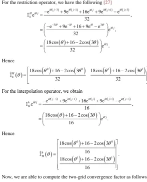
For the restriction operator, we have the following [27]

( ) ( ) ( ) ( )

( )

( )

3 1 1 3

3 3

e 9e 16e 9e e

e ,

32 e 9e 16 9e e

e , 32

18 cos 16 2 cos 3 e . 32

i j i j i j i j i j

H i j h

i i i i

i j

i j

θ θ θ θ θ

θ

θ θ θ θ

θ θ θ θ − − + + − − − + + + − = − + + + −  =     + −   =      Hence

( )

18 cos

( )

0 16 2 cos 3

( )

0 18 cos

( )

1 16 2 cos 3

( )

1

ˆ _.

32 32

H h

θ θ θ θ

θ = + − + − 

 

 



For the interpolation operator, we obtain

( ) ( ) ( ) ( ) ( )

( )

( )

3 1 1 3

e 9e 16e 9e e

e ,

16 18 cos 16 2 cos 3

e . 16

i j i j i j i j i j

h i j H

i j

θ θ θ θ θ

θ θ θ θ − − + + − + + + − = + −   =      Hence

( )

( )

( )

( )

( )

0 0 1 1

18 cos 16 2 cos 3 16

ˆ _.

18 cos 16 2 cos 3 16 h H θ θ θ θ θ  + −      =  _{+ −}        

Now, we are able to compute the two-grid convergence factor as follows



_{( )}

(

)

{

}

π 2

max H ,

TG TGh

θ

µ ρ θ

≤

= (5.12)

where ρ denotes the spectral radius of the 2 2× matrix TGH_h

( )

θ .

In Table 1, we report the values of the two-grid converge factor given by (5.12)

for different numbers of pre- and post-smoothing steps, ν ν₁, ₂. These values are computed by inspection of the function

(

H

( )

)

h

TG

ρ θ , which is evaluated using MATLAB to compute the eigenvalues of the matrix TGHh

( )

θ on a fine grid of

θ values, −π 2≤ ≤θ π 2.

Further in the same table, we compare these values with the value of the observed convergence factor given by

[image:13.595.213.508.75.439.2]

2 2 1 . h h m h _L m h _L r r ρ + =

Table 1. Estimated and observed multigrid convergence factors.

1, 2

ν ν _{1 2 3 4}

TG

µ _{2.000e−1 4.000e−2 8.000e−3 1.600e−3}

This numerical convergence factor represents the asymptotic ratio of reduction of the _L2_{-norm of the residual between two multigrid cycles. These calculations}

refer to the choice k x

(

−y

)

=exp

(

− −x y2

)

. As shown in Table 1, the LFA estimates of the multigrid convergence factor are accurate. (The same values of

TG

µ are obtained with L ranging from 20 to 400.)

6. Numerical Experiments

In this section, we present results of numerical experiments to validate our FAS-FI multigrid strategy and the theoretical estimates. We demonstrate that our FAS-FI scheme has 

(

MlogM

)

computational complexity (M denotes the total number of grid points on the finest grid) and provides second-order accurate solutions.

Our first purpose is to validate our accuracy estimates for the discretization scheme used. For this purpose, we consider an elliptic PIDE problem with a Gaus- sian convolution kernel in two dimensions as follows

( )

,

(

, , ,

) ( )

, d d

( )

, ,

u x y k x y t s u t s t s f x y

Ω Ω

−∆ +

_{∫ ∫}

= (6.1)

where Ω = −

(

1,1

) (

× −1,1

)

and the Gaussian kernel

(

, , ,

)

exp

(

) (

2

)

2

2

x t y s k x y t s = _− − + − _

 

.

To investigate the order of accuracy of the discretization scheme, we construct an exact solution to (6.1) by choosing

( )

2 2

, exp

2

x y u x y = _− + _

 . With this

choice, the right-hand side of (6.1) is given by

(

)

(

)

2 2 2 2

2 2

4 4

2

2 2 π

, 2 exp exp exp

2 4

2

erf 1 erf erf 1 erf 1 .

2 2 2 2

x y x y

x y

f x y x y

y y x x

    +  _{− + }

−  _{ }

   _{ }

   

 + 

= _− _− + +

 

    −      

×_{ } + _+ _{   } − _+ _ + _

       

   

The Dirichlet boundary is also given by the chosen u.

Using the exact solution above, we can validate the accuracy of our finite- differences and Simpson’s quadrature schemes. In Table 2, we report the values of the norm of the solution errors on different grids. We obtain second-order accuracy as predicted.

Next, we investigate the FI scheme. For this purpose, we consider the integral term in (3.3), and compute the norm h

h u− u

  . Notice that we can evaluate

u

 exactly, while hu is computed using the full-kernel (FK) evaluation formula (6) and the FI technique involving different depths,

d

= −

l

k

. For

d

=

0

the FI scheme performs FK evaluation.

In Table 3, we report the values of h

h u− u

[image:15.595.208.538.89.175.2]

Table 2. L2−norm error using full kernel approximation.

N×N u U− h order of accuracy

9 9× 8.60e−4 1.99 17 17× 2.16e−4 2.00 33 33× 5.41e−5 2.00 65 65× 1.35e−5 2.00 129 129× 3.38e−6

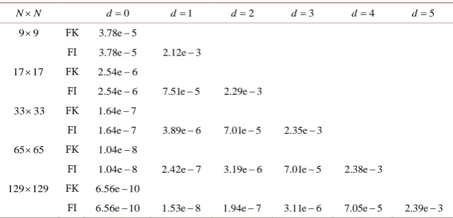
Table 3. Errors for 2D integral evaluation using 4th_{−order interpolation and different}

depths.

N×N d=0 d=1 d=2 d=3 d=4 d=5

9 9× FK 3.78e−5

FI 3.78e−5 2.12e−3 17 17× FK 2.54e−6

FI 2.54e−6 7.51e−5 2.29e−3 33 33× FK 1.64e−7

FI 1.64e−7 3.89e−6 7.01e−5 2.35e−3 65 65× FK 1.04e−8

FI 1.04e−8 2.42e−7 3.19e−6 7.01e−5 2.38e−3 129 129× FK 6.56e 10−

FI 6.56e 10− 1.53e−8 1.94e−7 3.11e−6 7.05e−5 2.39e−3

size and using the FK scheme. On the other hand, increasing the depth of the FI scheme, this scaling factor deteriorates. However, since the truncation error corre- sponding to the Laplace operator is of second-order, the reduction of accuracy due to the use of the FI scheme with the fourth-order quadrature does not affect the overall solution accuracy of the PIDE problem as shown in Table 4.

Next, we validate our FAS-FI solution procedure. One main issue is how the accuracy of the solution obtained with the FAS-FI scheme is affected by the approximation of the integral due to the FI procedure. For this purpose, in Table 4, we compare the norm of the solution errors obtained with a FAS scheme with FK calculation and with our FAS scheme including the FI technique. We see a moderate degradation of the quality of the numerical solution while increasing the depth. On the other hand, we notice that a second-accurate solution is obtained by choosing d corresponding to the first before the coarsest grid.

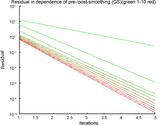
For the same experiments as in Table 4, we show large speed up in com- putational time in Table 5. Further, in Figure 1, we demonstrate that the compu- tational complexity of our multigrid procedure is 

(

MlogM

)

and M =N2 is the total number of grid points. In Figure 2, we depict the convergence history of the norm of the residuals at a given working level using different numbers of pre- and post-smoothing steps,

ν

=

1,



,10

, ν ν ν= +_{1 2}, and 5 V-cycle iterations. We complete this section, presenting results of experiments with a singular kernel, and consider an elliptic PIDE in one dimension of the following form

( )

log

( )

d

( )

u x x y u y y f x

Ω

[image:15.595.208.538.217.376.2]

[image:16.595.207.536.89.247.2]

Table 4. Errors of FAS solution with FK and FI integral evaluation after 5 V-cycles.

N×N d=0 d=1 d=2 d=3 d=4 d=5

9 9× FK 8.60e−4

FI 8.60e−4 8.39e−4 17 17× FK 2.16e−4

FI 2.16e−4 2.17e−4 2.06e−4 33 33× FK 5.41e−5

FI 5.41e−5 5.41e−5 5.51e−5 8.84e−5 65 65× FK 1.35e−5

FI 1.35e−5 1.35e−5 1.36e−5 1.46e−5 8.64e−5 129 129× FK 3.38e−6

[image:16.595.206.537.281.660.2]

FI 3.38e−6 3.36e−6 3.37e−6 3.45e−6 4.60e−6 8.88e−5

Table 5. CPU time (secs.) of FAS solution with 5 V-cycles. In bold are the values of CPU time actually involved in the multigrid solution scheme.

N×N d=0 d=1 d=2 d=3 d=4 d=5

9 9× FK 0.98

FI 0.95 0.53

17 17× FK 10.49

FI 10.36 3.27 1.72

33 33× FK 162.14

FI 161.41 44.33 15.78 8.63

65 65× FK 2568.89

FI 2574.11 731.88 224.03 84.37 47.75

129 129× FK 41970.15

FI 41939.82 11237.26 5378.64 1170.72 451.10 263.13

Figure 1. Computational complexity of the FAS-FI method; 2

M =N .

where f x

( )

=1 for x∈Ω = −:

(

1,1

)

. We further assume homogeneous Dirichlet boundary conditions.

has a singular kernel with one isolated singularity. On the singularity point, we cannot evaluate the kernel directly. However, we can estimate the integral using its values on neighbouring points. If the singularity is on one x_i of the grid, we use local averaging

( )

_{1 1}

2 2

1 2

i

i i

k x k x k x

− +

    

≈ _ _ _+ _ __

   

[image:17.595.229.516.209.427.2]

 . In Figure 3, we depict the observed multigrid computational complexity when solving the singular kernel problem and see that complexity appears to match or even improve on the typical estimate 

(

MlogM

)

. Further, in Figure 4 the convergence history of the

Figure 2. Convergence history of the FAS-FI scheme with different 1 2

ν ν ν= + , ν =1 (green) to ν =10 (red) along 5 V-cycles of FAS;

8, 3

[image:17.595.229.516.425.706.2]

l= d= .

[image:18.595.230.519.67.299.2]

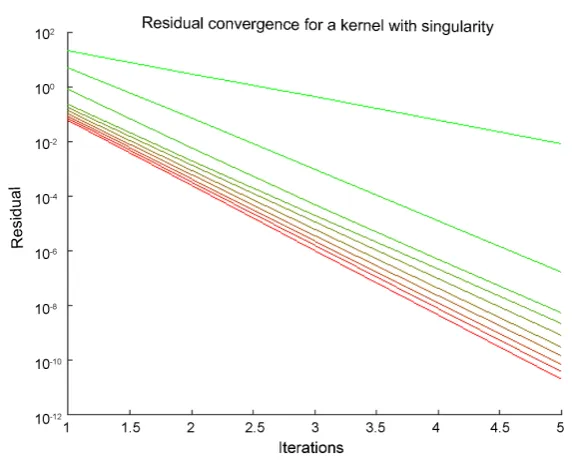
Figure 4. Convergence history of the FAS-FI scheme for a PIDE with singular kernel.

multigrid scheme with different pre- and post-smoothing schemes applied to the singular kernel case is presented.

7. Conclusion

An efficient multigrid finite-differences scheme for solving elliptic Fredholm par- tial integro-differential equations (PIDE) was developed and investigated. This scheme combines a FAS multigrid scheme for elliptic problems with a multilevel fast integration technique. Theoretical estimates of second-order solution accuracy and LFA multigrid convergence estimates were presented. These estimates were confirmed by results of numerical experiments.

Acknowledgements

This work was supported in part by the German Academic Exchange Service (DAAD), the European Union under Grant Agreement Nr. 304617 “Multi-ITN STRIKE-Novel Methods in Computational Finance” and by the Würzburg-Wro- claw Center for Stochastic Computing. This publication was funded by the Ger- man Research Foundation (DFG) and the the University of Würzburg in the fun- ding programme Open Access Publishing.

References

[1] Amstrong, N.J., Painter, K.J. and Sheratt, J.A. (2006) A Continuum Approach to Modelling Cell-Cell Adhension. Journal of Theoretical Biology, 243, 98-113.

https://doi.org/10.1016/j.jtbi.2006.05.030

[3] Hirsa, A. and Neftci, S.N. (2013) An Introduction to the Mathematics of Financial Derivatives. Academic Press, Cambridge.

[4] Itkin, A. (2016) Efficient Solution of Backward Jump-Diffusion Partial Integro-Di- fferential Equations with Splitting and Matrix Exponentials. Journal of Computa-tional Finance, 19, 29-70. https://doi.org/10.21314/JCF.2016.208

[5] Yaser, R. and Khosrow, M. (2017) Numerical Solution of Partial Integro-Differen- tial Equations by Using Projection Method Mediterranean. Journal of Mathematics, 14, 113.

[6] Thorwe, J. and Bhalekar, S. (2012) Solving Partial Integro Differential Equation Us-ing Laplace Transform Method. American Journal of Computational and Applied Mathematics, 2, 101-104. https://doi.org/10.5923/j.ajcam.20120203.06

[7] Ma, J., Jiang, Y. and Xiang, K. (2009) On a Moving Mesh Method for Solving Partial Integro-Differential Equations. Journal of Computational Mathematics, 27, 713- 728. https://doi.org/10.4208/jcm.2009.09-m2852

[8] Zhao, J. and Corless, R.M. (2006) Compact Finite Difference Method for Integro- Differential Equations. Applied Mathematics and Computation, 177, 271-288.

https://doi.org/10.1016/j.amc.2005.11.007

[9] Soliman, A.F., El-Asyed, A.M.A. and El-Azab, M.S. (2012) On the Numerical Solu-tion of Partial Integro-Differential EquaSolu-tions. Mathematical Sciences Letters, 1, 71- 80. https://doi.org/10.12785/msl/010109

[10] Liz, E. and Nieto, J.J. (1996) Boundary Value Problems for Second Order Integro- Differential Equations of Fredholm Type. Journal of Computational and Applied Mathematics, 72, 215-225. https://doi.org/10.1016/0377-0427(95)00273-1

[11] Volk, W. (1988) The Iterated Garlekin Method for Linear Integro-Differential Equ-ations. Journal of Computational and Applied Mathematics, 21, 63-74.

https://doi.org/10.1016/0377-0427(88)90388-3

[12] Hu, Q. (1998) Interpolation Correction for Collocation Solutions of Fredholm Inte-gro-Differential Equations. Mathematics of Computation, 67, 987-999.

https://doi.org/10.1090/S0025-5718-98-00956-9

[13] Volk, W. (1985) The Numerical Solutions of Linear Integro-Differential Equations by Projection Methods. Journal of Integral Equations, 9, 171-190.

[14] Hosseini, S.M. and Shahmorad, S. (2003) Tau Numerical Solution of Fredholm In-tegro-Differential Equations with Arbitrary Polynimial Bases. Applied Mathemati-cal Modelling, 27, 145-154. https://doi.org/10.1016/S0307-904X(02)00099-9

[15] Brandt, A. and Lubrecht, A.A. (1990) Multilevel Matrix Multiplication and Fast So-lution of Integral Equations. Journal of Computational Physics, 90, 348-370.

https://doi.org/10.1016/0021-9991(90)90171-V

[16] Heli, C.E. (2008) Real Analysis II. Georgia Institute of Technology, Atlanta. [17] Hackbusch, W. (1993) Elliptic Differential Equations Theory and Numerical Treat-

ment. Journal of Materials Science, 28, 5831-5835.

[18] Stoer, J. and Bulirsch, R. (2002) Introduction to Numerical Analysis. Texts in Ap-plied Mathematics, 79, 243. https://doi.org/10.1007/978-0-387-21738-3

[19] Jovanovic, B.S. and Süli, E. (2014) Analysis of Finite Difference Schemes. Springer Series in Computational Mathematics, 46, 198.

https://doi.org/10.1007/978-1-4471-5460-0

[20] Brandt, A. (1977) Multi-Level Adaptive Solutions to Boundary-Value Problems.

Mathematics of Computation, 31, 333-390.

[21] Trottenberg, U., Osterlee, C. and Schüller, A. (2001) Multigrid. Elsevier Academic Press, Amsterdam.

[22] Wesseling, P. (1991) An Introduction to Multigrid Methods. John Wiley and Sons, New York.

[23] Hemker, P.W. (1990) On the Order of Prolongations and Restrictions in Multigrid Procedures. Journal of Computational and Applied Mathematics, 32, 423-429.

https://doi.org/10.1016/0377-0427(90)90047-4

[24] Hackbusch, W. (1985) Multi-Grid Methods and Applications.Springer, Berlin.

https://doi.org/10.1007/978-3-662-02427-0

[25] Lubrecht, T. and Venner, C.H. (2000) Multi-Level Methods in Lubrication. Elsevier, Amsterdam.

[26] Brandt, A. (1982) Guide to Multi Grid Development. The Weizmann Institute of Science, Rehovot.

[27] Wienands, R. and Joppich, W. (1994) Practical Fourier Analysis for Multigrid me-thods. Chapman and Hall/CRC Press, Boca Raton.

Submit or recommend next manuscript to SCIRP and we will provide best service for you:

Accepting pre-submission inquiries through Email, Facebook, LinkedIn, Twitter, etc. A wide selection of journals (inclusive of 9 subjects, more than 200 journals)

Providing 24-hour high-quality service User-friendly online submission system Fair and swift peer-review system

Efficient typesetting and proofreading procedure

Display of the result of downloads and visits, as well as the number of cited articles Maximum dissemination of your research work

Submit your manuscript at: http://papersubmission.scirp.org/