Elasticity of substitution and technical progress: Is there a misspecification problem?

Munich Personal RePEc Archive

Elasticity of substitution and technical

progress: Is there a misspecification

problem?

Saltari, Enrico and Federici, Daniela

Department of Economics Law, Sapienza, University of Rome

13 December 2013

Elasticity of substitution and technical progress:

Is there a misspeci

_fi

cation problem?

∗

Daniela Federici

and Enrico Saltari

February 2014

Abstract

In Saltari et al. (2012, 2013) we estimated a dynamic model of the Italian economy. The main result of those papers is that the weakness of the Italian economy in the last two decades is due to the total factor productivity slowdown.

In those models the information and communication technology () capital stock plays a key role in boosting the efficiency of the traditional capital, and hence of the whole economy. The other key parameter to explain the Italian productivity decline is the elasticity of substitution.

Recent literature provides estimates of the elasticity of substitution well below 1 — thus rejecting the traditional Cobb-Douglas production function — though there is no particular value on which consensus converges. However, these estimates are affected by a theoretical specification problem. More generally, the technological parameters are long run in nature but the estimates are based on short-run data.

Our aim is to look more deeply into the estimation procedure of the techno-logical parameters. The standard estimation results present a common feature, a combination of a high-squared and serially correlated residuals, pointing towards a spurious regression bias. This bias is generated by a misspecification issue: the standard estimation approach is static in nature since do not incorporate frictions and rigidities.

Our modelling strategy takes into account, though implicitly, adjustment costs without leaving out the optimization hypothesis. Although we cannot in general say that this framework gets rid of the serial correlation problem, the statistics for our model do show that residuals are not serially correlated.

JEL classification: C30; E 22; E23; O33.

Keywords: CES production function; Elasticity of substitution; Income distri-bution; Factor-augmenting technical progress and ICT technical change.

∗_{We would like to thank Robert Chirinko, Giancarlo Gandolfo, Olivier de La Grandville and Clifford}

Wymer for their useful comments and suggestions. The usual disclaimer applies.

†_{University of Cassino and Southern Lazio. Email: [email protected].}

1

Introduction

In Saltariet al. (2012, 2013) we estimated a dynamic disequilibrium model of the Italian economy. The main result of those papers is that the weakness of the Italian economy in the last two decades has been the total factor productivity slowdown. To investigate the roots of this productivity decline, we drew attention to the reducing pace of capital accumulation. The model in both papers is based on the distinction between traditional and innovative capital. In a nutshell, our mainfinding shows that there exists a structural and persistent gap between "optimal" and observed output which, moreover, increased in the latter part of the sample period.

In those models two parameters play a crucial role. Thefirst is the capital stock, which is relevant in boosting the efficiency of the traditional capital and of labour, and hence of the whole economy. Formally, the  contribution is captured in a multiplic-ative way through a weighting factor. The other key parameter to explain the Italian productivity decline is the elasticity of substitution Since the introduction in the eco-nomic analysis by Hicks (1932) and its reformulation by Robinson (1933), the elasticity of substitution has attracted interest by both theoretical and empirical researchers for its central role in many fields such as economic growth, fiscal policy and development accounting. Recent analysis provides estimates consistently below 1 — thus rejecting the traditional Cobb-Douglas production function — though there is no particular value on which the consensus converged.

The estimation of these two parameters is however tricky. This is because they are long run in nature but their estimation is based on short-run data. In our opinion, the real issue is to bridge this gap. We will see that this problem has theoretical roots.

Economic literature has addressed this problem substantially in two ways. The first is based on statistical tools (such as cointegration,filtering, or simply assuming away the existence of the divergence) to recover long run technological parameters from the short run data. The second is to recognize the existence of short run adjustment problems and to model them either explicitly, e.g. as in the Tobin’s framework (see Chirinko 2008 for a comprehensive survey of both lines of research) or implicitly using ad hoc distributed lag processes not motivated by any form of optimization behavior. However, both methods are in some sense inappropriate in that they do not explicitly incorporate the dynamic effect of these costs on the factor inputs in estimating the elasticity of substitution.

Our aim in this paper is to look more deeply into the estimation procedure of the two technological parameters, the elasticity of substitution and the weight of ICT. We proceed in two steps.

In the first, we stay within the standard framework and run a number of estimates, using both single- and system-equation approaches. The estimation procedure employs normalization as an instrument which allows us to properly identify the deep technological parameters through a suitable choice of baseline point.

We begin with the single-equation approach in that we directly estimate the non-linear

gives an “unrealistic” value of the elasticity of substitution, we also estimate the weight of the capital. Our results show that single-equation approaches are largely unsuitable for jointly uncovering the elasticity of substitution and the weight of. We then build a system of two equations, the production function and the income share ratio derived from the two first-order conditions of the factor inputs.

This is the most popular estimation method. It is an approach based on two as-sumptions: there is an instantaneous adjustment of the marginal products to their user costs; it does not consider interactions with other markets. Within this framework, we get estimates for the elasticity of substitution and the weight of . However, the estimation results of these exercises present a common fundamental problem in that the error term is serially correlated so the standard errors will be under-estimated (i.e. biased downwards). At the root of this problem there is a specification problem: the estimated models are static in nature and do not incorporate frictions and rigidities. Thus, for instance, the production function is estimated without any correction for the costs of rigidities. The same holds for the estimation of income share ratio since it implicitly hypothesizes instantaneous adjustment between marginal products and input prices. Our model overcomes these difficulties by explicitly incorporating these costs.

The second step compares the results of our specification with those obtained from the standard estimation procedure

This comparison suggests that the more popular approach of using a system with instantaneous adjustment is biased: for example, the weight of  appears to be un-derestimated. Our model is based on the idea that firms optimize their intertemporal profits subject to the production function but taking account of rigidities, adjustment costs and other frictions. This produces a model which, at least to an approximation, enables the true parameters of the production function to be separated from the costs of adjustment, thus eliminating the autocorrelation in the residuals. The parameters then are not biased by those costs. When we take account of these costs, wefind an estimated elasticity well below unity, of about two-thirds.

The organization of the paper is as follows. The next section provides a brief literature review. Section 3 contains a short description of two issues related to the estimation of technological parameters. Section 4 gives the main empirical findings of our model. Section 5 "normalizes" the model and section 6 reports the results of the traditional approach to the estimation of the technological parameters. Sections 7 and 8 compare our estimation procedure with the standard one, offering some insights for the solution of the misspecification issue. Section 9 concludes.

2

Related Literature

substitution allows recognizing the existence of biased technical change (see Chirinko et al. 1999, Klump et al. 2008, León-Ledesmaet al. 2010). The wider use of CES technolo-gies opens the door to a deeper understanding of the effects of variation in the elasticity of substitution on economic growth (Turnovsky, 2002).

As pointed out by Nelson (1965), the elasticity of substitution can be interpreted as an index of the rate at which diminishing marginal returns set in as one factor is increased with respect to the other. If the elasticity of substitution is large, then it is easy to substitute one factor for the other. Therefore, the greater the elasticity of substitution the smaller the drag caused by diminishing returns. From this interpretation, it is straightforward to notice that the elasticity of substitution will affect the growth rate of output when factors of production are increasing at different rates so that their ratio is changing. The use of a Cobb-Douglas production function, as in most cases in the literature, is a misleading approximation for the behavior of the aggregate economy and hides the role of the elasticity of substitution not only as a source of increase in output but also as a source of technical change. If the elasticity of substitution in production is a measure of how easy it is to shift between factor inputs, typically labor and capital, it provide a powerful tool to answer questions about the distribution of national income between capital and labor.

The relevance of the elasticity of substitution and its relationship with economic growth and technical change has been established since Hicks (1932) and Solow (1957). However, it was after Arrow et al. (1961) that here was a boost on the theoretical and empirical issues involving the elasticity of substitution. More recently, La Grandville (1989) gives proof of the positive relationship between the elasticity of substitution and the output level. On the discussion about the theoretical and empirical role of the CES in the dynamic macroeconomics, see also Klump and Preissler 2000, Klump and La Grandville 2000, Klump et al. 2008 and La Grandville 2009.

Although the CES production technology seems relatively straightforward, its math-ematical simplicity can be misleading. La Grandville (1989), Klump and La Grandville (2000), Klump and Preissler (2000) and Klump et al. (2008) have emphasized that the economic interpretation of the CES production technology requires attention and they advocate the use of normalized production function when analyzing the consequences of variation in the elasticity of substitution. Normalization increases the usefulness of CES production functions for growth theorists, and this has led to its use in subsequent work such as Miyagiwa and Papageorgiou (2007) and Papageorgiou and Saam (2008). Nor-malization starts from the observation that a family of CES functions whose members are distinguished only by different elasticities of substitution need a common benchmark point. Since the elasticity of substitution is originally defined as point elasticity, one needs tofix benchmark values for the level of production, factor inputs and for the mar-ginal rate of substitution, or equivalently for per-capita production, capital deepening and factor income shares.1

3

Two relevant issues

Before addressing the technical aspect, we deem necessary to bring to attention two far-reaching features of the recent evolution of the economic environment of the main industrialised countries in the last decades, which are not only relevant by themselves but also because they affect the estimation robustness.

3.1

ICT role

Several recent studies have stressed the importance of 2 _{as a key factor behind the}

upsurge in the USA productivity after 1995 (see among others, Colecchia and Schreyer, 2001; Stiroh, 2002; Jorgenson, 2002). With regards to Europe, EU countries fall well below the United States in terms of  penetration (Timmer and van Ark, 2005). Whereas there exist a huge literature for the US economy, the literature is relatively scarce for Italy (see European Commission 2013). By now, it is an accepted fact that the setback of the Italian labour productivity in the last twenty years is explained by two factors: a marked slowdown of capital deepening accompanied by a striking negative contribution of TFP.

To go a step further, notice that these two phenomena go hand-in-hand and are both relevant in explaining the standstill of labour productivity. Capital accumulation is important because, as is well known at least since Solow (1957), most of technical progress is embodied in new capital goods. In fact, what the data about capital deepening show is that in the Italian economy during the last 15 years there occurred a shift towards less capital intensive techniques, thus reducing the efficiency of employment. This shift and the lack of adoption of new technologies, especially of the ICT variety, have been favoured by the particular structure of the Italian specialization, skewed towards the traditional sectors with low technological content and less skilled workers. That is, not only the investment pace decreased in the last 15 years but it was also redirected toward traditional sectors rather than the innovative ones. Such a change in capital accumulation mix explains why both TFP and capital intensity rates decreased at the same time.

To confirm this last point, it is enough to have a look at the Figure 1, where the capital input growth rates for the total economy, the  and the non- sectors are depicted.

Figure 1 Capital accumulation in Italy (growth rates percent)

The figure makes clear two aspects of the trend of capital accumulation in Italy. The first is that the dynamics of total capital accumulation mostly follows that of capital accumulation in the traditional (non ICT) sector: the two lines essentially go hand-in-hand. The second is that the investment rate in the  sector accelerates up to the end of 1980s, and then slows down, albeit with a recovery in the mid-1990s. Notice that it becomes negative in the most recent years.

The contribution of the  sector to the productivity dynamics has not been mod-elled. The bulk of the literature assumes that technical progress grows at a constant rate without giving a specific structure within which the  does play any role (a partial exception is Klump et al. 2008). In our model we take a stance about how impacts on technical progress: particularly, we assume that the productivity of the traditional capital stock is augmented by the  capital stock. This makes a difference with re-spect to the traditional approach in that the effect of  is not constant but reflects the pace of investment in innovative technologies.

3.2

The decline of labour share

was approximately constant in almost all the countries thus confirming one of the stylized fact highlighted by Kaldor (1961).

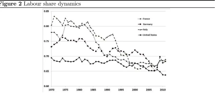
Figure 2 Labour share dynamics

The figure (2) shows that up to the 70s the stationarity of factor share is more or less confirmed. However, starting from the following decade the decline of labor share becomes evident: for the period 1980-2011 the reduction is 11 per cent for Italy and France, 8 per cent in Germany, and 6 per cent in the USA. Obviously, this downward trend will not last forever. It seems that in the past thirty years the income shares dynamics has been (at least locally) nonstationary; in other words, it is likely that this process will come to a halt. The local nonstationarity will create problems since it is an independent source of serial correlation. As far as we know, this is a critical issue which is not taken into account in the estimation of the technological parameters of the production function, and especially in that of the elasticity of substitution. Though this is a relevant question, it is not clear which kind of way out can be adopted.

4

Our model

there are imperfections and frictions.3

Let us have a look at the second order (time) derivative of the log of traditional capital which implicitly defines the investment equation in our model, repeated here for the reader’s convenience:

˙

 = 1

∙

2 µ



 − ( − 7ln + 8) ¶

−(−_)

¸

where  =ln () ˙ =2_{ln () and}

 is the growth rate of labor efficiency. Inside the parentheses, we model the adjustment of the marginal product of capital to its user cost, defined by the real interest rate plus a risk premium (₈). The speed at which firms make this adjustment is given by2or, in other words, how long it takes to adjust the existing capital stock to its desired level. As time goes by, however, this desired level changes at the velocity_ Inside the square brackets we find this second long run adjustment process, which runs at1, the speed of the accumulation process. Of course, as the estimates in Saltariet al. (2012) confirm, thefirst adjustment takes a much shorter time than the second one.

All the other equations in our model are specified in a similar manner, i.e. as dynamic equations. This implies that the model is recursive in the sense that it is expressed as a system of differential equations in which the derivative of each endogenous variable depends on the levels of all the other variables.4

Formally, these assumptions give rise to a system of stochastic differential equations which is estimated by the full-information maximum likelihood method ( ). It is important to note that the parameters of the production function occur throughout the model in the various marginal product conditions that arise from cost minimisation. The way in which they occur varies with the specific marginal functions. 5

The aggregate production function (·) is given by:

 =3 h

( 1)−1 +

¡

2

¢ −1i −_1

1 (1)

3_{The adjustment process may take two forms. First-order process assume that the variable under}

consideration adjust to its partial equilibrium level in the following way

() =[ˆ()₋()]

whereˆ()is the equilibrium or desired level,is the speed of adjustment and is the operator. Second-order adjustment assume instead that it is the rate of change of the variable to adjust to its equilibrium level

2

() =1{2[ˆ()−()]−()}

where thefirst term in parenthesis describes the adjustment of the variable to its desired level.

4_{More details on these dynamic disequilibrium models can be found in Gandolfo (1981) and Wymer}

(1996).

5_{The  estimator used ensures that all of the cross-equation constraints implicit in these}

In equation (1) _ = +1 is the growth rate of labor efficiency and  and  are the rates of technical progress in the use of traditional capital stock and innovative capital. These terms may be interpreted as an indication of the expected long-run term rates of growth, providing the system is stable. The coefficient₂ is the labor augmenting technical progress, while ₃ is a measure of the total factor productivity. The efficiency of traditionalfixed capital stock is augmented by capital,, with a weighting factor equal to ₁; the elasticity of substitution is 1 = ₁₊1_1.

Defining as a Cobb-Douglas function of the skilled and unskilled labor components,

the production function can be written as:6

 =3 h

( 1)−1 + ¡ 2

¢ −₁i ₋ 1

_{1 (3)}

Two features of the production function (3) are worth noticing. First, as emphasized above, the specification of factor-augmenting technical progress is based on the key role played by  on the productivity dynamics in industrialized countries since 90s. The

 relevance is particularly important for Italy, although in a negative sense. However, as demonstrated in Diamond et al. (1978), it is impossible to separately identify this role from that of the elasticity of substitution unless one imposes a specific structure of technical change. In defining this structure, we abandon the traditional specification of technical progress growing at a constant rate. This is the second feature of the produc-tion funcproduc-tion. Our model assumes that the efficiency of traditional fixed capital stock is augmented by capital according to a weighting factor equal to ₁ Since the labour augmenting index is defined as  =  +1 this same factor also increases the efficiency of labour. That way, we are assuming that  investment improves labour productivity. Hence, we explicitly introduce the capital stock as a capital augment-ing efficiency factor which also affects the labour-augmenting efficiency factor. To our knowledge, this specification of technical progress was first introduced in Kaldor (1957) growth model.7

6_{This production function can be easily transformed into the well know form introduced in the}

liter-ature by Arrow et al.(1961):

= h

(1)−1 + (1−) ¡

2_

¢−1i − 1

1 (2)

where the “efficiency” parameter is defined as  = 3

 1+−1

2

1

1

and the “distribution” parameter as

= 1

1+−1 2



7_{He is explicit in affirming that one specific characteristic of his growth model is that: “... it eschews}

4.1

Estimation results

As a consequence, the parameters of the production function are not the result of a single-equation estimation, equation (3). Rather, they are obtained by the estimation of a structural dynamic model of general and investment functions, skilled and unskilled labour sectors, and price determination under imperfect competition (see Appendix for a description of the complete model).8 _{The parameters’ estimates of the production}

functions are reported in Table 1.

Table 1 Parameter Estimates

(asymptotic standard errors in parenthesis)

₁ 1 2 3 1    

0519

(00045) 0(0658020) 27(3598)075 0(0869031) 0(0048013) 0(0027005) 0(0971010) 0(0001001) 0(0036005)

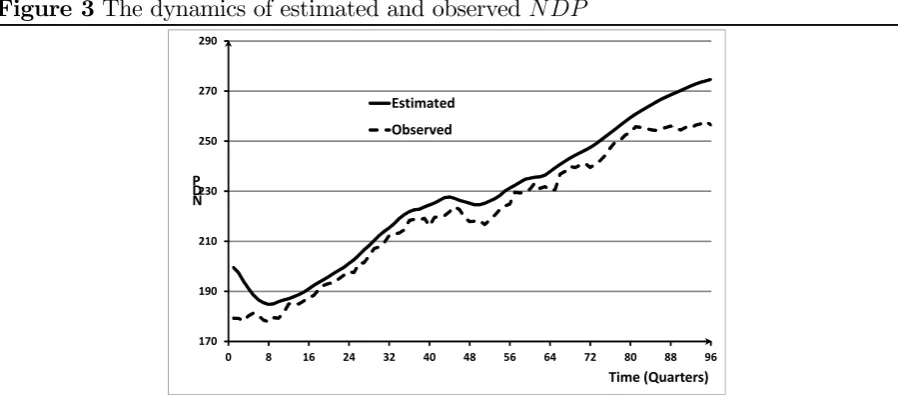
The estimated Italian national domestic product () for the period 1980:Q2— 2005:Q1, a total of 100 quarters9 _{is reproduced, together with the actual one, in figure}

3.

The whole system of nonlinear stochastic differential equations allow us to estimate the production function (or production frontier) subject to all the constraints mentioned above. The estimated parameters of the production function gives the output at any given levels of inputs. It is the amount of output that would be achieved, in equilibrium, if the levels of inputs were used efficiently on the production frontier.

A visual inspection of the figure reveals that the model replicates pretty well what happened in Italy in the period under observation (the correlation coefficient is 0.99). However, a persistent gap exists between the estimated and observed dynamics of the Italian  which tends to widen towards the end of the sample period. On average over the sample period, the quarterly gap between the estimated and observed  is about 3 per cent.

8_{The model assumes that the market environment is one of imperfect competition wherefirms have}

similar production functions but different endowments and their products are sufficiently differentiated that they are monopolistic competitors in the short run, setting their own prices. Thus they may set prices according to their marginal costs plus some mark-up or margin. As a consequence, each firm is assumed to be a “quantity-taker” and aims to supply the amount demanded.

Figure 3 The dynamics of estimated and observed

170 190 210 230 250 270 290

0 8 16 24 32 40 48 56 64 72 80 88 96

N D P

Time (Quarters) Estimated

Observed

Our estimation of the elasticity of substitution (1 = 0658) is confirmed by recent econometric studies.

These contributions find values of 1 that are consistently below unity, but a great deal of variation in the results persists. Pereira (2003) surveyed major papers in thefield from the past 40 years and found that,in general, elasticity values were below unity. A recent survey by Chirinko (2008) looked at modern studies of the elasticity parameter and found considerable variation in cross-study results. However, the weight of the evidence suggested a range of 1 that is between 0.4 and 0.6, with the assumption of Cobb-Douglas being strongly rejected. Klump et al. (2008) estimated a long-run supply model for the euro area over the period 1970-2005 and they found an aggregate elasticity of substitution below unity (around 0.7). Mallick (2012) obtained the elasticity parameters for 90 countries by estimating the CES production function for each country separately using respective country time series spanning for the period 1950—2000. The mean value for all 90 countries is 0.338. The mean values for the East Asia and Sub-Saharan African countries are 0.737 and 0.275, respectively. For the  countries the mean is 0.340. A clear pattern is evident, he concludes, that, on average, the value of elasticity increases secularly with the growth rate of per capita. One problem with interpreting these cross-study results is that the various analyses are not all measuring the same thing: the results found are generally sensitive to sample size and estimation techniques. La Grandville (1989), Klump and La Grandville (2000) emphasize the role of normalization of the CES production function because it makes more consistent cross-study estimates of the elasticity parameter.

5

Normalization

Following Klump and La Grandville (2000) and Klump and Preissler (2000), we “nor-malize” the production function. The normalization procedure identifies a family of CES production functions that are distinguished only by the elasticity parameter.10

Normaliz-ation is a way to represent the production function so that the variables are independent of the unit of measure, i.e. in an index number form. This makes the parameter estimation easier.11

To begin with, we set the base period used for the normalization at the middle of the sample,= 48corresponding to 1993:Q3. To simplify notation, we denote this period by the index 0 Normalization implies that all the variables are expressed in terms of their baseline values, that is0 0 and0

To normalize the production function, we start with the production function:

 =3 h

( ) −1 + ¡ 2(−0)

¢ −1i −_1

1 (4)

where 0 is the base period and, to simplify notation, we set  = 1.

Under imperfect competition, factor compensation is subject to a mark-up, by hy-pothesis constant and denoted by ₁₃12 _{so that in any period  the following relation}

holds:

(+)13= where  is the real interest rate and  is the wage rate.13 In the reference period capital compensation is:

0 =

1

₁₃ 0 0

= (3) −₁

₁₃ µ

0 0

¶1+1

10_{Klump and Saam (2008) emphasize that normalization is necessary to avoid “arbitrary and}

incon-sistent results.”

11_{It should be emphasized that while the normalization issue is useful in an analysis of the properties}

of the production function and of importance in some estimation, it does not affect the estimates of our model. In this model, the specification of the equations being estimated are such that models with different normalizations are stochastically equivalent. Once one has consistent estimates of the parameters (as in the FIML case), the functions may be viewed in other ways for analysis. It does not affect their properties.

12_{A margin over and above the input marginal products is the traditional way to include the markup.}

An alternative is Rowthorn (1999), which adds the extraprofit from market power into the capital income share. We choose the former since formally it is the easiest way to take into account the existence of imperfect competition.

13_{The wage rateis given by:}

()

 = 

_+ 

_

Similarly, the unit capital compensation is:

()

 = (−ln+8)



 + (−ln+10)

 

so that total capital compensation over total factor income, or the capital share, in the base period is

0 =

00 0

13 = (3)−

₁µ 0 0

¶1

(5)

Likewise, the labor compensation in the base period is

0 =

1

13 0 0

= (32) −1

13 µ

0 0

¶1+1

so the labour share is

1−0 = 00

0

₁₃= (₃)−1

µ 0 ₂0

¶1

(6)

Notice that labour share expressed in efficiency units is simply 2 since in the base period the time-dependent efficiency factor disappears.

Substitute into the production function (4) the capital share evaluated in the base period: = " 0 µ 0 0

¶−₁

()−1 +¡32 (−0)¢

−1

#− 1 1

Following an analogous procedure for the labor share (6), we have:

 =0 "

0 µ



0 ¶−₁

+ (1−0) µ

 (−0)

0

¶−₁#−11

(7)

In the index number form, the production function is:

 0 = " 0 µ  0 ¶−₁

+ (1₋0) µ

 (−0)

0

¶−₁#−11

(8)

For simplicity, this last equation will be rewritten as:

 =

h

0()−1 + (1−0)¡ (−0)¢− ₁i−1₁

(9)

In the capital intensive form with inputs expressed in efficiency units the equation be-comes



 (−0)

 = " 0 µ  (−0)



¶−₁

+ (1₋0) #−1₁

normalized production function the only key parameter is ₁ which is related to the elasticity of substitution, 1.

Before performing any estimation exercise using normalization, we need tofix income shares in the benchmark period. Employing observed data for capital, labour and output and our parameters estimates of table 1, the capital share for the Italian economy, see equation (5), is:

0 = (3)−

1

µ 0 0

¶1

= 024

so that labour income share is

1−0 = 076

Since these estimates are quite close to those present in different databanks (such as OECD, EU KLEMS, AMECO), we adopt these shares for the reference period.

6

Estimation results

6.1

Single-equation approach

The single-equation approach has been used for parameters estimation following two alternative routes: the production function and the optimizing behavior present in the equations of the income shares. We discuss these two estimation directions in the following subsections.

6.1.1 Technology

Let us begin with the estimation of the production function (9). We first estimate only

₁ setting the other parameters (₁  ) at their values in table (1), with nonlinear least squares. Specifically, we used the production function in log form:

ln () =−

1 ˆ

1

lnh0− ˆ

1

 + (1−0) (−0)− ˆ

1



i

where ˆ₁ is the estimated value

This produces an estimate equal to ˆ₁ = 89 The implied value of the elasticity of substitution is ˆ1 = _1+ˆ1_

1 = 01which has an R-squared equal to 098 Notwithstanding

the high significance level and the goodfit, this estimates presents at least two problems. First, the implied level of1is quite low and “unrealistic”. Second, and more importantly, the Durbin-Watson statistics is very low ( = 019) indicating the existence of serial correlation in the residuals.14 _{The strong residual autocorrelation invalidates the }ˆ

1 estimate.

14_{Here, and in what follows, we tested for residual correlation computing and Breusch-Godfrey}

As we saw above,  played a key role in explaining the Italian economic dynamics. Hence, we try to fix the specification problem extending the estimation to the weight of

. Consequently, we jointly estimate the elasticity of substitution and the role of

in increasing the efficiency of traditional capital. This gives rise to estimates, ˆ₁ = 116

andˆ₁ = 0037 with an R-squared equal to 098. This slightly increases the estimate of

ˆ

1 — the elasticity of substitution becomesˆ1 = 008— but the serial correlation remains high ( = 024).

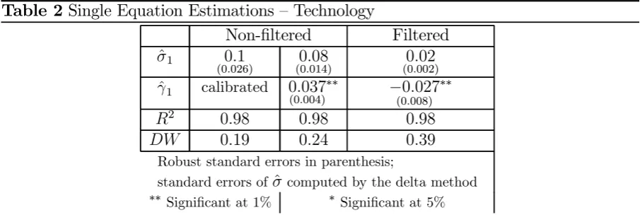
Up to now we estimated the parameters using the observed variables, without taking into account that the estimation refers to long run relations. One of the methods fre-quently used in the literature to recover “desired” or long run values is to filter the time series.15 _{The adopted procedure transform variables in the frequency domain excluding}

medium and high frequencies, keeping only low frequencies. In the time domain this al-lows to get long run variables. So, what do we get from filtering? We tried several filters — the Baxter-King and Christiano-Fitzgerald versions, with different hypothesis about the trend — but results seem insensitive to these transformations. These are ˆ1 = 493 (ˆ1 = 002) and ˆ1 = −0027 (which is implausible). However, the  weight has an implausible negative sign and, above all, the residual are still serially correlated.16

Table 2 Single Equation Estimations — Technology

Non-filtered Filtered

ˆ

1 01

(0026) (00014)08 (00002)02

ˆ

₁ calibrated 0037

(0004)

∗∗ _−0027

(0008)

∗∗

2 _{098 098 098}

 019 024 039

Robust standard errors in parenthesis;

standard errors ofˆcomputed by the delta method ∗∗_{Significant at 1%} ∗ _{Significant at 5%}

It is worth noticing that all these regressions have a common feature; they present a combination of a low and a high R-squared. This combination, which will recur in all the subsequent regressions, seems to suggest a spurious relation between variables.

The problem with estimating a production function as a single equation is that it assumes that output is on the production frontier. It may also have a simultaneous equation bias since it assumes that throughout the sample, output is determined by the supply side only. However, it is likely that the last few years have shown that output is demand driven. If so, however, it isthat is causingandnot vice versa. Separately from all of that, although the representation and estimation of a production function is important, on its own it is a purely technical relation.

15_{Filtering methodologies results, in this case, in a reduction of the sample period to 1984Q4-2002Q3.} 16_{We also replicated the specification of Mallick (2012), who assumes Hicks-neutral technical progress,}

In addition, the approach of trying to adjust the explanatory variables,  and , withfiltering techniques, loses information and may leave one not knowing what is really being lost. Also, the standard errors of the parameters of the estimated production function are usually incorrect as they are based on the adjusted or filtered values of  and, not the actual ones.

6.1.2 Income shares

Let us now turn to the estimation of thefirst-order conditions related tofirm’s optimizing behavior. We use the income share equations which embody the first-order conditions. In writing the production function in its index form, we employed the mid-sample as a reference period. Income shares at the baseline value were determined as follows:

1−0 = (3)−

₁µ 0 ₂0

¶1

More generally, the labour share in period  can be written as:

1₋= (3)−

1

µ



2 (−0)

¶1

where _ = +1 Dividing side by side the last two equations, we obtain

1− = (1−0) µ



_ (−0)



¶1



This equation has a straightforward economic interpretation: the labor income share is directly related, via₁ and thus the elasticity of substitution, to the productivity of labor expressed in efficiency units.

Taking logs of the last expression, we get:

ln (1−) = ln (1−0) +1ln µ



_(−0)



¶

 (10)

As in the case of production function estimation, we set the lambdas at the values specified in Table 1 and estimate the two deep parameters ₁ and 1 Using both observed and filtered data for the variables involved in the previous equation, we get almost the same values for ₁ equal to 02 (ˆ1 = 083), whereas the weight of ICT is 039 for unfiltered data and042for thefiltered ones. What remains unchanged is the high serial correlation in the residuals.

An analogous estimation can be done for the capital income share. The equation estimated is:

=0 µ



1

¶

and in log form:

ln () = ln (0) +1ln µ



1

As in the case of labour, the capital income share is directly linked to the productivity of capital expressed in efficiency units through the capital contribution. Estimating this equation as above with observed and “long run” data, we obtain a value for 1 equal to 381 (ˆ1 = 021) for the former and ˆ1 = 114 (ˆ1 = 047). What appears counterintuitive in both cases is the sign of the estimated₁which is negative. However, this is a finding not uncommon in the literature (see for instance Antras 2004). The estimate of the elasticity of substitution based on the labour income share is higher that based on capital income share, an empirical regularity confirmed also in other studies.

Finally, we estimate the ratio of income shares:



1−

= 0 1−0

µ_ (−0)_



1

¶₁

and in log form:

ln

µ 

1−

¶

= ln

µ 0

1−0 ¶

+₁ln

µ

_ (−0)_



1

¶ 

In words, the ratio of capital to labour income share is inversely related to labour-capital ratio, both expressed in efficiency units. Figure 2 does not support one of more accepted stylized facts in economic literature, the stationarity of income shares. In the sample period considered, there has been a continuous increase in the capital share — not only in Italy but, as the figure shows, in most industrialized countries. Even if the profit share seems to be stabilized at a new level in recent years, it creates an estimation problem which is not easy to solve (see the results in table 3). In fact, we made attempts, both with raw andfiltered data, to deal with this problem without obtaining satisfactory results: for instance, the estimated weight of is implausibly high (above 40%, while the weight of the  capital stock in the total capital stock is in the range of 3-6%). Moreover, the residuals remain serially correlated.

Table 3 Single Equation Estimations — Income shares (robust standard errors in parenthesis)

Labour income share Capital income share Income Share ratio Non-filtered Filtered Non-filtered Filtered Non-filtered Filtered

ˆ

1 083

(01) (00015)83

∗ _021

(0056)

∗∗ _047

(0131)

∗∗ _133

(065) (005802)

∗∗

ˆ

₁ 039

(024) 042

∗∗

(005) −(00028)16

∗∗ _−053

(014)

∗∗ _046∗∗

(012) (006104)

∗∗

2 _{074 094 066 080 088 095}

 001 003 007 002 003 003

Robust standard errors in parenthesis; standard errors ofˆcomputed by the delta method

∗∗_{Significant at 1%} ∗ _{Significant at 5%}

 and a high R-squared. As is well known, in this case the estimates are consistent only if there exists a cointegrating relationship. In all the previous regressions we tested for this possibility — using different hypothesis on trend specification.17 _{We were not}

able to obtain unambiguous results since the presence of a cointegrating relation very much depends on the number of lags included. In our opinion, these findings suggest a misspecification issue.

The problem behind the one-equation approach — such as =( )alone — is that it assumes the observations are taken from a static economy in equilibrium. We can see no way that can hold. These three variables are perhaps the most heavily inter-related in theory: both  and  will be functions of demand, and demand (for given prices and wages) must be met from domestic output, imports or variations in stocks.  will depend on some investment function which alone will lead to lags. will depend almost certainly on demand and the current (installed) production frontier, so even leaving aside simultaneous equation bias, there will be some form of serial correlation (probably moving average disturbances) within the model. Similar problems arise in the context of income share estimation.

6.2

System approach

Since the single equation approach seems unsuitable for jointly estimating the two tech-nical parameters of interest, we turn our attention to the system approach, which is also the most frequently used in the literature.

The system estimated is:

⎧ ⎨ ⎩

ln () =−_ˆ1

1 ln

h

0−ˆ1 + (1−0) (−0)− ˆ

₁ 

i

ln³ 

1−

´

= ln³ 0

1−0

´

+₁ln³(−0)_

1

´ (11)

We estimated (11) using non-linear SUR. The estimation of this system gives wrong signs for both parameters and strongly indicates the presence of serial correlation (the

 is close to 0). The residual autocorrelation is confirmed by the multivariate Box-Pierce/Ljung-Box Q-statistics. To correct for this problem, we decide to add autore-gressive components. We run unit root tests both for the  and the income share ratio, indicating that the former is (1) while the latter is (2) This leads to include one autoregressive term in the first equation of the system and two in the second equa-tion. The estimation procedure reduces, but does not solve, the serial correlation in the residuals; furthermore, it gives a wrong sign in the ˆ₁ estimate.18 _{A look at the residual}

correlogram drives to increase the number of autoregressive terms in the equation of the income share ratio. Increasing the order of the autoregressive process partly solves the serial correlation problem but the economic content of this econometric manipulation has very limited value.19

17_{We used Engle-Granger and Phillips-Ouliaris single-equation residual-based cointegration tests.} 18_{The strategy offiltering data does not improve the results.}

7

The theoretical roots of the estimation problem

As seen above, the traditional approach has some weaknesses. Indeed, a key issue arises in estimating the technological parameters. To see the problem at hand in the simplest way, suppose that the production function underlying the economy may be represented as =(  ) where is a vector of parameters. These are technological parameters indicating the way in which factors of production are brought together to produce output. If the economy has frictions, rigidities etc. which reduce the efficiency of production, these rigidities must be taken into account in the estimation of the parameters of the production function for, otherwise, the standard errors of the estimates will be biased. Some of those rigidities will be unavoidable; it takes time to install capital, build a new plant, etc., but it can be assumed firms will take whatever steps they can to minimize costs associated with those rigidities. The same will apply to regulations; althoughfirms are assumed to minimize costs by choosing the optimal point on the production frontier, depending on factor costs, rigidities will encourage or force the firm to operate at some other, sub-optimal point. This sub-optimal point may be at a different point on the same “iso-technology” frontier or the whole frontier may be sub-optimal.

If data were available on costs, it might be possible to build these into the production function but generally that is not the case at the aggregate level anyway. Also, to the extent thatfirms take steps to reach the optimal position from their current sub-optimal position, estimation of the production function is likely to result in auto-correlated errors. The divergence between sub-optimal and optimal variables is often cast in terms of the difference between observable short run data and their long run values. Observable data do not include adjustment costs while the long run values — on which the estimates should be based — are already cost adjusted but are unobservable.

The divergence between optimal and sub-optimal positions is a problem with time-series analysis; auto-correlated errors are often eliminated statistically but if they have an economic cause originating from a misspecification problem, the model should be re-specified accordingly. The estimated model should be based on the idea that firms optimize their intertemporal profits subject to the production function but taking account of rigidities, adjustment costs and other frictions. This produces a structural dynamic model which, at least to an approximation, enables the true parameters of the production function to be separated from the costs of adjustment. The parameters  then are not biased by those costs.

Our model is based on the idea that firms optimize their intertemporal profits sub-ject to the production function but taking account of rigidities, adjustment costs and other frictions. This produces the dynamic model which, at least to an approximation, enables the true parameters of the production function to be separated from the costs of adjustment. The parameters then are not biased by those costs.

Once the model specified to include these costs has been estimated, so if the specific-ation is correct, the parameters will be unbiased, the partial equilibrium of the economy

may be calculated under the assumption that costs of rigidities are zero. Observations of economic variables include these costs (so output would be higher if these costs did not ex-ist), while the calculated values from the unbiased estimates exclude them so (estimated) output in the latter case should be higher than observed.

A more formal way of looking at this from a general point of view, is to think of a theoretical function

˜

() =(() ) +() (12)

where the () are a set of errors that would arise if this relationship, and in particular

˜

(), could be observed. This relationship could then be estimated directly.

If this relationship is subject to adjustment costs, rigidities, frictions etc., the function above could be considered as embedded in a more general relationship, for instance

() =[(() ) () ] +() (13)

which may depend on other variables()and parameters, which gives a better repres-entation of the economy. Thus()is the variable, corresponding to˜()that is observed. In that case, it is this second equation that should be estimated for all of the parameters

 . If this second equation is the correct specification of the model that produces the observed () estimating the first equation on the assumption that ˜() = () would produce biased estimates of the parameters vector . Thus () is the variable corres-ponding to that observed. In that case, it is equation (13) that should be estimated for all of the parameters .

If (13) were the true model but (12) is estimated using the observed values of()it is likely that residuals in (12) will then be serially correlated. Take for instance the behavior of factor markets. These are very often characterized by frictions and rigidities arising from many sources that affect adjustment process. In many countries, the employment protection legislation is evidence of the existence of institutional factors that delay or hinder the achievement of equilibrium in the labor market; at the same time, they make the wage unresponsive to the excess of demand or supply. Similarly, the optimal or “desired” capital stock cannot be instantaneously obtained given a variety of adjustment costs. Some scholars (see, for example, Antras 2004, Leon-Ledesma et al. 2010) do not consider the presence of those frictions and rigidities assuming that the economic system is in equilibrium at any point in time. Although this assumption may be convenient for theoretical work, it causes an error in the specification of the structure underlying the model thus giving rise to serially correlated residuals.

As this has an economic cause, that is it is due to a misspecification of using ()

with (12) rather than (13), it should be eliminated by using the correct specification rather than by some statistical means. Because of the dynamics in the true model, if we wished to use values calculated from (13) to re-estimate (12) directly, we would need to calculate “observations” of these variables from (13) first, but such estimates would almost certainly be inconsistent.20 _{In the following we will see that the standard approach}

suffers from such a misspecification problem.

20_{As all the FIML or similar estimators are asymptotic, a vector of parameters is consistent if and}

8

The misspeci

_fi

cation problem

Our model is formulated as a dynamic disequilibrium system in continuos time. The model is based on the idea thatfirms optimize their intertemporal profits subject to the production function but taking account of rigidities, adjustment costs and other frictions. This produces the dynamic model which, at least to an approximation, enables the true parameters of the production function to be separated from the costs of adjustment. The parameters then are not biased by those costs.

Once the model specified to include these costs has been estimated, so if the specifi c-ation is correct, the parameters will be unbiased, the partial equilibrium of the economy may be calculated under the assumption that costs of rigidities are zero. Observations of economic variables include these costs (so output would be higher if these costs did not ex-ist), while the calculated values from the unbiased estimates exclude them so (estimated) output in the latter case should be higher than observed.

These particular features may help, at least in principle, in solving the residual cor-relation and misspecification problems seen above. As the reader may recall, the misspe-cification derives from the "fundamental tension", as Chirinko (2008) dubs it, between the short run observable data and the long run nature of the elasticity of substitution. As the estimation results showed, the ways out of this problem proposed in the literature have not been useful. Our modelling strategy takes into account, though implicitly, a variety of adjustment costs without leaving out the optimization hypothesis. Turning again to the accumulation equation, the alphas embody the adjustment lags with which thefirm reach their optimal capital stock.

The standard procedure assume instead there are no lags or frictions hampering the equality between input prices and their marginal products in estimating the technical parameters.

One may ask what results would be obtained following the standard procedure. there are two main points characterizing the traditional methodology of estimating the elasticity of substitution and technical change. First, because of the impossibility of identifying the parameters separately, it is imposed a specific structure on technical progress: it is assumed that the factor input efficiency grows at a constant growth rate. Second, it is assumed that the adjustment speed of the factor marginal productivities at their rental prices tends to infinity. Antras (2004) is perhaps one of the best recent paper that exemplifies the standard approach.

His main result is that the elasticity of substitution is well below 1, and hence the aggregate production function is not of Cobb-Douglas type. However, from the very beginning he has to deal with the problem emphasized above, i.e. a combination of high R-squared and low Durbin-Watson statistics pointing out towards a spurious regression bias. To solve this problem, he employs a number of econometric techniques (besides

,   and cointegration) without substantial improvements.

Assumingfinite adjustment speed and a different form of technical change, in our opin-ion, provides a better representation of the economic system. Although our framework cannot always guarantee the solution to the specification problem, in this case it turns out that residuals are not serially correlated. Multivariate Portmanteau or  (Ljung-Box) statistic is equal to 101.4 for thefirst two autocorrelations.21 _{As a consequence, the}

null hypothesis that the residuals are not serially correlated cannot be rejected because the  statistic is below the critical value in the region of the upper tail.22 _{This is not a}

surprising result since a second order differential equation model gives rise to a second order moving-average error process that is taken into account explicitly in the estimation procedure. To the extent that observations generated by a second order system inher-ently incorporate a first or second order moving average process depending on whether the variables are stocks or flows, at least in a linear model and to an approximation in a non-linear model, that too can be taken into account and the variables transformed to remove the serial correlation (see Wymer, 1972).

9

Conclusions

A growing number of papers has shown that the elasticity of substitution is a key tech-nological parameters for boosting economic efficiency. Perhaps the most innovative and interesting result of this literature is that the elasticity of substitution well below 1, i.e. the Cobb-Douglas assumption is biased upward.

However, in our opinion these new estimates are affected by a theoretical weakness. The elasticity of substitution is a long run technological parameter whose estimation is constrained by the availability of short run data. This problem has been solved employ-ing two different econometric strategies: on the one hand, making use of a theoretical framework to account for the delayed adjustment to the long run optimizing relationship; on the other,filtering the data in such a way to retain only long run components.

This paper has emphasized that these estimates have a serial correlation problem deriving from unsolved theoretical issues: it is difficult to explicitly specify the appropriate adjustment costs and datafiltering are subject to the usual ad-hock criticism. The model we proposed is a tentative solution strategy to these problems in that it incorporates frictions and, as a disequilibrium model, it is intrinsically dynamic. The test results seem to confirm that our strategy is effective.

A distinguished feature of our model is the capital-augmenting technical progress which gives a key role to the ICT capital stock, differently from the existing literature where it is generally assumed constant. The next step of our research project is to extend the model by endogenizing the ICT sector.

21_{Augmented Dickey-Fueller statistic may also be run for the single equations of the model. Although}

these are not appropriate for a FIML estimator, the single equation results, for what they are worth, show no relevance to non-linear differential equation systems.

22_{Approximate critical values of Chi-Square distribution with 98 degrees of freedom are at 5 per cent}

References

Acemoglu, D. (2008): Introduction to Modern Economic Growth, MIT Press. Aghion P., and P. Howitt (2009): The Economics of Growth, MIT Press.

Antràs, P. (2004), "Is the US Aggregate Production Function Cobb-Douglas? New Estimates of the Elasticity of Substitution". Contributions to Macroeconomics, 4, Issue 1, Article 4.

Arrow, K.J., Chenery, H.B., Minhas, B.S., Solow, R.M., (1961):" Capital-labor sub-stitution and economic efficiency". The Review of Economics and Statistics 43, 225—250. Basu, S., and D. Weil (1998): "Appropriate technology and growth", Quarterly Journal of Economics, 113, 1025-54.

Bergstrom, A. R. (1984): "Monetary, fiscal and exchange rate policy in a continuous time model of the United Kingdom", in P. Malgrange and P. Muet, eds., Contemporary Macroeconomic Modelling. Oxford: Blackwell, 183-206.

Bergstrom, A. R., K. B. Nowman, and C. R. Wymer, (1992): “Gaussian estimation of a second order continuous time macroeconometric model of the United Kingdom”.

Economic Modelling, 9, 313-351.

Bergstrom, A. R., and K. B. Nowman, (2006): “A Continuous Time Econometric Model of the United Kingdom with Stochastic Trends”. Cambridge: Cambridge Univer-sity Press.

Bergstrom A. R. and C. R. Wymer (1976): “A model of disequilibrium neo-classical growth and its application to the United Kingdom”, in A. R. Bergstrom, ed., Statistical Inference in Continuous-Time Economic Models. Amsterdam: North-Holland, 267-328.

Chirinko, R. (2008): ": the long and short of it", Journal of Macroeconomics, 30 (2): 671-686.

Chirinko, R., S. M. Fazzari, A. P. Meyer, (1999):" How responsive is business capital formation to its user cost? An exploration with micro data". Journal of Public Economics

74 (October), 53—80.

European Commission (2013): Towards Knowledge Driven Reindustrialisation, European Competitiveness Report.

Colecchia, A. and P. Schreyer (2001), “The Impact of Information Communications Technology on Output Growth”, STI Working Paper 2001/7, OECD, Paris.

Diamond, P. , D. McFadden and M. Rodriguez (1978), “Measurement of the Elasticity of Factor Substitution and Bias of Technical Change,” in M. Fuss and D. McFadden (eds), Production Economics: A Dual Approach to Theory and Applications (Volume 2), Amsterdam: North-Holland, 125-147.

Elsby, M. W. L., B. Hobijn, A. ¸Sahin (2013), “The Decline of the U.S. Labor Share”, mimeo.

Gandolfo, G. (1981): Qualitative Analysys and Economteric Estimation of Continuous Time Dynamic Models, North-Holland.

Hicks, J. R., (1963): The Theory of Wages, second ed. MacMillan & Co., London (first edition published in 1932).

Jorgenson, D., M. S Ho, and K. J Stiroh (2004). “Will the U.S. Productivity Resur-gence Continue?”. Current Issues in Economics and Finance 10, no. 13, 1-7.

Kaldor, N. (1957), “A Model of Economic Growth”, Economic Journal, 67, 591-624. Kaldor, N. (1961), “Capital Accumulation and Economic Growth,” in F.A. Lutz and D.C. Hague, eds., The Theory of Capital, St.Martins Press, 177—222.

Karabarbounis, L. and B. Neiman (2013):"The Global Decline of the Labor Share", mimeo.

Klump R., P. McAdam and A. Willman (2008):"Unwrapping some euro area growth puzzles: Factor substitution, productivity and unemployment",Journal of Macroeconom-ics, 30 (2): 645-66.

Klump R., P. McAdam and A. Willman (2012): " The Normalized CES Production Function: Theory and Empirics",Journal of Economic Surveys, 26, 769 - 799.

Klump R. and O. de La Grandville (2000): “Economic growth and the elasticity of substitution: Two theorems and some suggestions”,The American Economic Review, 90, 282-91.

Klump R. and H. Preissler (2000): “CES Production Functions and Economic Growth”,

Scandinavian Journal of Economics, 102, 41-56.

Klump, R. and Saam, M. (2008): "Calibration of normalised CES production func-tions in dynamic models", Economics Letters, Elsevier, 99(2), 256-259.

Knight, M. D. and C. R. Wymer (1978): “A macroeconomic model of the United Kingdom”. IMF Staff Papers, 25, 742-78.

La Grandville, O. de (1989): "In quest of the Slutsky diamond", American Economic Review, 79, 468-481.

La Grandville, O. de (2009): Economic Growth: A Unified Approach. Cambridge: Cambridge Cambridge University Press.

León-Ledesma, M. A., P. McAdam and A. Willman (2010):" Identifying the Elasti-city of Substitution with Biased Technical Change", The American Economic Review, 100(4):1330—1357.

Miyagiwa, K. and Papageorgiou, C. (2007): "Endogenous aggregate elasticity of sub-stitution", Journal of Economic Dynamics and Control, vol. 31(9), 2899-2919.

Nelson, R. R. (1965):" The CES Production Function and Economic Growth", The Review of Economics and Statistics, Vol. 47, No. 3, 326-28

Mallick, D. (2012):"The role of the elasticity of substitution in economic growth: A cross-country investigation", Labour Economics 19 (2012) 682—694.

Papageorgiou C. and M. Saam (2008): "Two-level CES Production Technology in the Solow and Diamond Growth Models", Scandinavian Journal of Economics, 110(1), 119-143.

Pereira, C. (2003). “Empirical Essays on the Elasticity of Substitution, Technical Change, and Economic Growth.” Ph.D. dissertation, North Carolina State University.

Rowthorn R. (1999) :"Unemployment, Capital-Labor Substitution, and Economic Growth", Cambridge Journal of Economics, 23, 413-425.

Saltari, E., C. Wymer, D. Federici and M. Giannetti (2012), "Technological adop-tion with imperfect markets in the Italian economy, Studies in Nonlinear Dynamics & Econometrics, 16, 2.

Saltari, E., C. Wymer and D. Federici. (2013). "The impact of ICT and business services on the Italian economy, Structural Change and Economic Dynamics, 25, 110— 118.

Solow, R. (1957): "Technical change and the aggregate production function", Review of Economics and Statistics, 39, 312-320.

Stiroh, K. J. (2002): "Information Technology and the U.S. Productivity Revival: What Do the Industry Data Say?",The American Economic Review, 92(5), 1559-1576.

Timmer, M.P. and van Ark, B. (2005):" Does information and communication tech-nology drive EU-US productivity growth differentials?", Oxford Economic Papers, 57(4), pp. 693—716.

Turnovsky, S. J. (2002):" Intertemporal and intratemporal substitution and the speed of convergence in the neoclassical growth model", Journal of Economic Dynamics and Control,26, 1765—1785.

Wymer, C. R. (1972): "Econometric estimation of stochastic differential equation systems", Econometrica, 40, 565-77.

Wymer, C. R. (1996): “The role of continuous time disequilibrium models in macroe-conomics”, in Barnett, W.A., G. Gandolfo and C. Hillinger, eds.,Dynamic Disequilibrium Modeling, Cambridge: Cambridge University Press.

Wymer, C. R. (1997): "Structural non-linear continuous-time models in economet-rics", Macroeconomic Dynamics, 1, 518-48.

Appendix A

The core of the model is composed by the following seven differential equation (for more details, see Saltari et al. 2012):

1. Investment functions:

(a) Traditional capital

˙

 = 1

∙

2 µ_

 − ( − 7ln + 8) ¶

−(−)

¸

(A.1)

(b) ICT capital

˙

=3

∙

4 µ



 − ( − 9ln  + 10) ¶

−( ₋ _)

¸

(A.2)

where in Equation (A.1)_ =+(−1)+and in Equation (A.2)

 =+23

2. Skilled labour:

(a) Demand for skilled labour

˙

= 5

∙

6 ln µ   Á   ¶

+ 0

6 ln µ    Á   ¶ − ( − ) ¸ (A.3)

(b) Skilled wages

2ln = 7[8 ln µ     ¶

+0

8ln µ      ¶ −

(7 +8+08) (ln − 11 ln−  −1) ] (A.4)

where₁₁ measures money illusion.24

3. Unskilled labour:

(a) Employment

˙

 =910 ln ¡¢ − (9+10) ( − ) (A.5)

23_{While the investment equations allow for money illusion in specifing the real interest rate, estimates}

showed that7and9 were not significantly different from 1 and in thefinal estimates they were set to 1.

24_{Estimates of }

(b) Unskilled wages

2ln  = 11

∙

12 ln µ     ¶

− (ln 

 −  − 1) ¸

(A.6)

where 

 = 0 ³





´12

_{ In the model, changes in the unskilled labor}

supply depend on the real wage, with elasticity12. Thus, the effect on labor supply will be largely symmetrical at the margin for increases and decreases of real wages. However this is only one side of the labor market. We should also take into account the demand side. Unless the elasticity of real wages in the supply function is one, changes in nominal wages have a differing effect on prices and hence on real wages. The price effect then feeds back into invest-ment, capital, and thus on the demand for labour via its marginal product.

4. Price determination:

The marginal cost of labour is obtained in the usual way as a ratio between the mean wage and the marginal product of labour, where labour is defined as a Cobb-Douglas function of the two labor components, = 

  The short term marginal cost is a weighted average of skilled and unskilled wage rates

 µ   ¶ = µ   +   ¶ −

 −(23)− 1

−(+1)h_{1 +}¡_

2(+1) ¢1i

1+1 ₁

where =_₁

The dynamics of price determination are described by a second-order process:

2_{ln() =} 15ln

Ã

₁₃ ¡ 

¢



!

+13 µ ln µ   ¶ − ¶ +

+14 ½ ln µ   ¶

−(+1)

¾

+16ln ½

 

¡

1 +−−¢

¾

(A.7)

where ₁₃ is the mark-up and ¡ 

¢

is the marginal cost determined as follows. Further,= ln+ ln −ln is the mean velocity over the sample and is assumed to vary at a rate

 =7 h

−6 _{+ (}

8exp())−6