Testing for the buffered autoregressive processes

Testing for the buffered autoregressive

processes

Zhu, Ke and Yu, Philip L.H. and Li, Wai Keung

Institute of Applied Mathematics, Chinese Academy of Sciences,

Department of Statistics and Actuarial Science, University of Hong

Kong, Department of Statistics and Actuarial Science, University of

Hong Kong

25 November 2013

Online at

https://mpra.ub.uni-muenchen.de/51706/

PROCESSES

By Ke Zhu, Philip L.H. Yu and Wai Keung Li

Chinese Academy of Sciences and University of Hong Kong

This paper investigates a quasi-likelihood ratio (LR) test for the thresholds in buffered autoregressive processes. Under the null hypothesis of no threshold, the LR test statistic con-verges to a function of a centered Gaussian process. Under local alternatives, this LR test has nontrivial asymptotic power. Fur-thermore, a bootstrap method is proposed to obtain the critical value for our LR test. Simulation studies and one real example are given to assess the performance of this LR test. The proof in this paper is not standard and can be used in other non-linear time series models.

1. Introduction. After the seminal work of Tong (1978), threshold autoregres-sive (TAR) models have achieved a great success in practice; see, e.g., Tong (1990) for earlier works and Tong (2011) and the references therein for more recent ones. Generally speaking, the TAR model says that the structure of an AR model shifts among different regimes, i.e.,

yt=φ0+ p

X

i=1

φiyt−i+

Ã

ψ0+ p

X

i=1 ψiyt−i

!

Rt+εt, (1.1)

where Rt =I(yt−d ≤ r) is the regime indicator of yt, r is the threshold parameter,

d(_≥ 1) is the delay parameter, and εt is an uncorrelated error sequence with zero mean and varianceσ2(>0). There have been a lot of interests to detect the threshold in TAR models since 1990s. Chan (1990, 1993) and Chan and Tong (1990) first accomplished this task by considering a likelihood ratio (LR) test for TAR models. Moreover, Tsay (1989) gave some novel methods in this context; Hansen (1996) studied the Wald test and Lagrange multiplier (LM) test for TAR models; Wong and Li (1997, 2000) studied LM test for TAR-ARCH models; Li and Ling (2013) investigated the portmanteau test for threshold double AR models; see also Tsay (1998), Hansen (1999), Caner and Hansen (2001), Ling and Tong (2005), Li and Li (2008, 2011), and Zhu and Ling (2012).

Keywords and phrases: AR(p) model, Bootstrap method, Buffered AR(p) model, Likelihood ratio test, Marked empirical process, Threshold AR(p) model.

Under model (1.1), the regime of yt shifts when the state of yt−d changes. In practice, the regime of ytmay not shift immediately, and there could be a buffering region in which the regime of yt depends on the regime ofyt−d. Li, Guan, Li, and Yu

(2012) first formulated this situation by assuming that Rt in model (1.1) satisfies

Rt =

      

1 if yt−d≤rL

0 if yt−d> rU

Rt−1 otherwise ,

(1.2)

whererLandrU are two threshold parameters such thatrL ≤rU. They called model (1.1)-(1.2) the buffered AR (BAR) model, and the region in which yt−dlies between

rL andrU is called the buffering region. Also, they found that the BAR model is the best selected model for the sunspot series in Tong (1990) and GNP series in Tiao and Tsay (1994), and hence it may provide us with a new way to understand the non-linear time series. However, how to test for BAR models is still unknown, and it is more challenging than testing for TAR models because the regime of yt in this case depends on past observations infinitely far away.

In this paper, we investigate a quasi-LR test for the thresholds in BAR mod-els. Under the null hypothesis of no threshold, the LR test statistic converges to a function of a centered Gaussian process. Under local alternatives, this LR test has nontrivial asymptotic power. Our result nests the one in Chan (1990) as a special case, but its proof is not standard and different from the proof in that paper. Fur-thermore, a bootstrap method is proposed to obtain the critical value for our LR test. Simulation studies and one real example are given to assess the performance of this LR test.

This paper is organized as follows. Section 2 states our main result on the LR test. Section 3 proposes a bootstrap procedure. The simulation results and one real ex-ample are given in Section 4. The proofs are provided in the Appendix, which can be found in Zhu, Yu, and Li (2013). Throughout the paper, some symbols are conven-tional. _|A_| = (tr(A′

A))1/2 _{is the Euclidean norm of a matrix A. kAk}

s = (E|A|s)1/s is the Ls_{-norm (s ≥ 1) of a random matrix. A}′

2. Likelihood ratio test. Let φ = (φ0,_{· · ·} , φp)′

, ψ = (ψ0,_{· · ·} , ψp)′

, λ = (φ′

, ψ′

)′

,γ = (rL, rU), and xt= (1, yt−1,· · · , yt−p) ′

. Then, model (1.1)-(1.2) becomes

yt =xt(γ)′λ+εt, (2.1)

wherext(γ) = (x′

t, ht(γ)

′

)′

,ht(γ) =xtRt(γ), andRt(γ) is defined as in (1.2). Here, we assume that all the roots of the characteristic equationφ(x) =xp_−φ1xp−1_{− · · · −φ}

p lie inside the unit circle, and both p and d are known. Without loss of generality, we further assume that d _≤p if p_≥1, because we can setp=d with φp+1 =· · ·= φd= 0 andψp+1 =· · ·=ψd= 0 in (2.1) when d > p≥1.

Suppose that _{y0,_{· · ·} , yN} are N + 1 consecutive observations from model (2.1) with the true parameters λ0 and γ0, where λ0 = (φ′

0, ψ ′ 0)

′

, φ0 = (φ00,_{· · ·}, φp0)′, ψ0 = (ψ00,_{· · ·} , ψp0)′, and γ0 = (rL0, rU0). We consider the following hypotheses:

  

H0 :ψ0 = 0,

H1 :ψ0 ₆= 0 for some γ.

(2.2)

Model (2.1) is an AR(p) model underH0 and it is a buffered AR(p) (BAR(p)) model under H1. When rL = rU (i.e., the buffering region is absent), (2.2) is for testing the threshold in the threshold AR(p) (TAR(p)) model, for which the likelihood ratio (LR) test was studied by Chan (1990, 1991) provided thatεt∼N(0,1) is a sequence of i.i.d. random variables. When rL 6=rU, since

Rt(γ) =I(yt−d ≤rL)

+

∞

X

j=1

I(yt−j−d≤rL) j

Y

i=1

I(rL< yt−i+1−d≤rU) a.s., (2.3)

we can see thatRt(γ) depends on all past observations infinitely far away. Note that

Rt(γ) in Chan (1990) only depends on yt−d. Thus, the test in Chan (1990) is not a LR test any more and may be less powerful in this case. Motivated by this, we consider an alternative LR test for (2.2).

Denote Y = (yp,· · · , yN)′ and Zγ = (X, Xγ) =

³

xp(γ), xp+1(γ),· · · , xN(γ)

´′

, where

X = (xp, xp+1,· · · , xN)′,

Xγ =

³

hp(γ), hp+1(γ),· · · , hN(γ)

´′ .

Let n=N ₋p+ 1 be the effective number of observations. Following Chan (1990), we know that for any fixed value of γ, the LR test statistic is

LRn(γ) = n[σ

2

n−σn2(γ)]

σ2

n

where

σ_n2 = 1

n{Y ′

Y ₋(Y′ X)(X′

X)−1_(X′ Y)_},

(2.4)

σ_n2(γ) = 1

n{Y ′

Y ₋(Y′

Zγ)(Z′

γZγ)

−1_(Z′

γY)}. (2.5)

Since the exact value ofγ is unknown underH0, it is natural to construct the LR test by using the maximum of LRn(γ) over the range ofγ; see Davis (1977, 1987). Thus, our LR test statistic is defined as

LRn= sup

γ∈ΓLRn(γ),

where Γ _{≡ {}(rL, rU);a≤ rL ≤rU ≤ b} and [a, b] is a predetermined interval. Here, we truncate the full range of γ, since LRn may diverge to infinity in probability as

n _{→ ∞}; see Andrews (1993a).

Let Kγδ = E[xt(γ)xt(δ)′]. To study the asymptotic theory of LRn, we need the following three technical assumptions:

Assumption 2.1. yt is strictly stationary, ergodic and absolutely regular with

mixing coefficients β(m) = O(m−A

) for some A > v/(v ₋ 1) and r > v > 1;

E_|yt|4r<∞, E|εt|4r <∞; and Kγγ is positive definite.

Assumption 2.2. yt has a bounded and continuous density function.

Assumption 2.3. There exists an A0 >1 such that 2A0rv/(r−v)< A.

Assumptions 2.1-2.2 are from Hansen (1996), in which the weak convergence of empirical process is derived by using the method in Doukhan, Massart, and Rio (1995). When Pp

i=1|φi| < 1 and Pip=1|φi +ψi| < 1, Li, Guan, Li, and Yu (2012) showed that model (2.1) is strictly stationary and ergodic. Assumption 2.3 is needed to prove Lemma A.1 in the Appendix. When A > v/(v₋1), a sufficient condition for Assumption 2.3 is thatv <3r/(2r+ 1), which is stronger thanv < ras required in Assumption 2.1. Particularly, whenεtis a sequence of i.i.d. random variables with a bounded and continuous density function, β(m) decays exponentially underH0 as

shown in Pham and Tran (1985). Thus, the mixing condition of yt in Assumption 2.1 and also Assumptions 2.2-2.3 hold in this case.

Furthermore, we state two key lemmas, under which a uniform expansion of

Lemma 2.1. If Assumptions 2.1-2.3 hold, then (i) it follows that

sup γ∈Γ

¯ ¯ ¯ ¯ ¯ ¯ ¯

  

X′

γXγ

n −

X′

γX

n

Ã

X′ X n

!−1

X′ Xγ

n

  

−1

−(Σγ₋ΣγΣ−1Σγ)−1¯¯

¯=op(1); (ii) furthermore, under H0 it follows that

sup γ∈Γ

¯ ¯ ¯ ¯ ¯

Tγ−

³

−ΣγΣ−1_{, I}´ 1

√ nZ

′

γε

¯ ¯ ¯ ¯ ¯

=op(1),

where ε = (εp,· · · , εN)′, Tγ = n−1/2

n

X′

γ−X

′

γX(X

′

X)−1_X′o

Y, Σ = E(xtx′t), and Σγ =E[xtx′tRt(γ)].

Proof. See the Appendix in Zhu, Yu, and Li (2013).

Lemma 2.2. If Assumptions 2.1-2.3 hold, then it follows that

1

√ nZ

′

γε ⇒σGγ

as n _{→ ∞}, whereGγ is a Gaussian process with zero mean function and covariance

kernel Kγδ.

Proof. See the Appendix in Zhu, Yu, and Li (2013).

Note that

1

√ nZ

′

γε = 1

√ n

N

X

t=p (x′

t, x

′

tRt(γ))

′ εt.

We call_{n−1/2_Z′

γε}a marked empirical process as in Stute (1997), where eachyt−i−d in Rt(γ) is a marker. In view of (2.3), we know that _{n−1/2_Z′

γε} involves infinitely many markers, and this is also the case when Ling and Tong (2005) studied the LR test for TMA models. However, their method seems hard to be implemented in our case. Compared with the proof of Lemma 2.1 in Chan (1990) or Ling and Tong (2005), the proofs of Lemmas 2.1-2.2 in the Appendix are not standard and can be used in other non-linear time series models.

We are now ready to present our main result as follows:

Theorem 2.1. If Assumptions 2.1-2.3 hold, then under H0 it follows that

LRn →d sup γ∈Γ

G′

γΩγGγ

as n_{→ ∞}, where Ωγ = (−ΣγΣ−1, I)

′

(Σγ−ΣγΣ−1Σγ)

−1

Proof. By (2.4)-(2.5) and a direct calculation, we have

nhσ2_n−σ_n2(γ)i

=T′

γ

  

X′

γXγ

n −

X′

γX

n

Ã

X′_X n

!−1 X′_X

γ

n

  

−1

Tγ. (2.6)

By Lemmas 2.1-2.2, the conclusion follows directly from the same argument as for Theorem 2.3 in Chan (1990).

Remark 2.1. Note that

G′

γΩγGγ =ξ′γ

³

Σγ−ΣγΣ−1Σγ

´−1 ξγ,

where ξγ = (−ΣγΣ−1, I)Gγ. Then, by a direct calculation, we can easily show that

for each γ _∈ Γ, G′

γΩγGγ follows a χ2 distribution, namely, for fixed γ, the test

statistic LRn(γ) is asymptotically pivotal under H0.

Remark 2.2. Although the result in Theorem 2.1 nests the one in Theorem 2.3(ii) of Chan (1990) as a special case, it is necessary to mention some difference between our LR test and that in Chan (1990). First, the denominator of LRn(γ) in our case is different from that in Chan (1990), but we can easily show that these two denominators are asymptotically equivalent; see also Ling and Tong (2005). Second, since the region of Γ is larger than that in Chan (1990), our LR test needs more computational efforts than that in Chan (1990).

Remark 2.3. As Chan (1990), we only obtained the result under the condition that V ar(εt) =σ2_{. The case that the threshold effect happens in the variance of ε}

t

needs a further study in the future.

Next, we study the asymptotical local power of LRn by considering the following local alternative hypothesis:

H1n :ψ0 =

h √

n for a constant vector h∈ R

p+1_.

Theorem 2.2. If Assumptions 2.1-2.3 hold, then under H1n it follows that

LRn→dsup γ∈Γ

n

G′

γΩγGγ+h′µγγ0h

o

,

as n_{→ ∞}, where Mγγ0 =E[xtx

′

tRt(γ)Rt(γ0)] and

µγγ0 = 1

σ2

³

Mγγ0 −ΣγΣ−1Σγ

´′³

Σγ₋ΣγΣ−1_Σγ´−1³

Mγγ0 −ΣγΣ−1Σγ

´

Proof. Note thatY =Xφ0+Xγ0h/√n+ε under H1n. Thus,

Tγ = 1

√_nnX_γ′ ₋X_γ′X(X′

X)−1_X′o ε+ 1

n

n

X_γ′ ₋X_γ′X(X′

X)−1_X′o Xγ0h

= _√1

n

³

−(X′

γX)(X

′

X)−1_{, I}´

Z′

γε+ 1

n

n

X_γ′ ₋X_γ′X(X′

X)−1_X′o Xγ0h.

By (2.6) and Lemmas 2.1-2.2, the conclusion follows directly from the same argument as for Theorem 2.3 in Chan (1990).

In practice, the values ofa andb can be set to empirical quantiles of _{yt}Nt=0 as in

Chan (1991) and Andrews (1993b), although so far how to choose the optimal a, b

remains unclear in theory. In this case, we can always find a smallestn0 _≥psuch that

yn0−d stays outside the region [a, b], where the integer n0 depends on data sample

{y0,_{· · ·} , yN}. This means that we can observe Rn0(γ), and then further calculate

{Rt(γ)_}N

t=n0+1 iteratively by

Rt(γ) =I(yt−d≤rL) +Rt−1I(rL< yt−d≤rU).

For the remaining observations _{yt}n0t=0−1 whose regions are not well identified, we

then set their regions to be 0. Thus, we can only use ˜Rt(γ) rather than Rt(γ) in practice, where

˜

Rt(γ) =

  

0 for t= 0,_{· · ·} , n0₋1, Rt(γ) for t=n0,_{· · ·} , N.

(2.7)

Let ˜LRnbe defined in the same way asLRnwithRt(γ) being replaced by ˜Rt(γ). The following corollary shows that ˜LRn and LRn have the same asymptotic property.

Corollary 2.1. If Assumptions 2.1-2.3 hold, then (i) under H0 it follows that

˜

LRn →dsup γ∈Γ

G′

γΩγGγ as n → ∞;

(ii) under H1n it follows that

˜

LRn →dsup γ∈Γ

n

G′

γΩγGγ+h′µγγ0h

o

as n _{→ ∞}.

3. Bootstrapped critical value. In this section, we use a bootstrap method to obtain the critical value for our LR test; see also Hansen (1996) and Li and Li (2011). First, we let

ˆ

εt=yt−xt(γ)′λn(γ) (3.1)

with

λn(γ)_≡arg min λ∈Λ

N

X

t=p

ε2_t(λ, γ) = hZ′

γZγ

i−1h

Z′

γY

i

,

where Λ is a compact parametric space of λ, and εt(λ, γ) = yt−xt(γ)′λ. Next, we set

ˆ

LRn(γ) = Zˆ ′

n(γ)(X1n(γ), I)′[X2n(γ)]−1(X1n(γ), I) ˆZn(γ)

σ2

n

,

(3.2)

where ˆε= (ˆεpvp,· · ·,εˆNvN)′,{vt}Nt=p is a sequence of i.i.d.N(0,1) random variables, and

ˆ

Zn(γ) = 1

√ nZ

′

γε, Xˆ 1n(γ) = −

X′ γX

n

Ã

X′

X n

!−1

,

and X2n(γ) = X ′ γXγ

n −

X′ γX

n

Ã

X′

X n

!−1

X′

Xγ

n .

Define

ˆ

LRn≡sup γ∈Γ

ˆ

LRn(γ).

(3.3)

The asymptotic theory of ˆLRn is stated in the following theorem:

Theorem 3.1. If Assumptions 2.1-2.3 hold, then under H0 or H1n, it follows

that

ˆ

LRn|y0,· · ·, yN →dsup γ∈Γ

G′

γΩγGγ in probablity as n→ ∞.

Proof. See the Appendix in Zhu, Yu, and Li (2013).

Remark 3.1. In practice, LRˆ n is calculated withRt(γ)being replaced by R˜t(γ).

Note that the conditional limiting distribution in Theorem 3.1 is the same as the null distribution in Theorem 2.1. Then, conditional on the data sample _{y0,_{· · ·} , yN}, for any given significance level α, we use the following bootstrap procedure to obtain our critical value:

(i) generate i.i.d. N(0,1) samples_{vt}Nt=p, and then calculate ˆLRn via (3.1)-(3.3); (ii) repeat step (i) for J times to get _{LRˆ (1)_n ,_{· · ·} ,LRˆ (_nJ)_};

(iii) choose cJ

n,α be the α-th upper percentile of {LRˆ

(1)

n ,· · · ,LRˆ

(J)

n }. From now on, we choose cJ

n,α as the critical value for our LR test, i.e., at the signif-icance levelα, ifLRn ≥cJn,α, we reject H0; otherwise, we accept it. In Section 4, we

shorten cJ

n,α as cn for brevity.

In the end, we give a critical corollary as follows:

Corollary 3.1. If Assumptions 2.1-2.3 hold, then (i) under H0 it follows that

lim

n→∞_Jlim→∞P

³

LRn≥cJn,α

´

=α;

(ii) under H1n it follows that

lim

h→∞nlim→∞_Jlim→∞P

³

LRn≥cJn,α

´

= 1.

Proof. See the Appendix in Zhu, Yu, and Li (2013).

Corollary 3.1 guarantees that our bootstrapped critical valuecJ

n,αis asymptotically valid, and our LR test has power to detectH1n. This method is also feasible to obtain the critical value for the LR test in Chan (1990) by settingγL≡γU. Moreover, since

ˆ

LRn(γ) is a step-function, the amount of computation on cJ

n,α depends only on the effective sample size n and the bootstrapped sample sizeJ. Hence, this will reduce our computational burden significantly in application.

4. Simulation and one real example. In this section, we first compare the performance of our LR test (LRn) and Chan’s (1990) LR test (LR∗

n) in the finite sample. We generate 1000 replications of sample size n = 200 from the following BAR model:

yt=yt−1−0.09yt−2+ (ψ1yt−1+ψ2yt−2)Rt(γ) +εt, (4.1)

where Rt(γ) is defined as in (1.2) with d = 1, εt has N(0,1) distribution, and the initial values y0 = y1 = R1(γ) = 0. We choose γ = (0,0), (0,0.5), (0,1.5) or

is (0.1,0.9) in the regime of Rt(γ) = 0, we choose (ψ1, ψ2) = (0,0), (0.1,₋0.09), (0.3,₋0.27), (0.5,₋0.45) or (0.7,₋0.63) such that the pair of characteristic roots in the regime of Rt(γ) = 1 is (0.1,0,9), (0.2,0.9), (0.4,0.9), (0.6,0.9) or (0.8,0.9), respectively. For each replication, the value ofaandb for the interval [a, b] are set to be the empirical 10th and 90th quantiles of data sample, the critical value for LRn is calculated by the bootstrap method in Section 3 with J = 1000, and the critical value for LR∗

n is either calculated in the same way as the one for LRn or taken as 15.18 according to Table 2 in Chan (1991).

Table 1

Rejection rates

ψ γ LR∗

n

ψ1 ψ2 rL rU LRn LR∗1n LR∗2n

0.0 0.0 — — 4.9 4.9 3.4

0.1 -0.09 0.0 0.0 7.7 7.7 3.8 0.0 0.5 7.5 7.4 3.7 0.0 1.5 7.6 6.5 3.2 0.0 2.0 7.5 7.0 5.4 0.3 -0.27 0.0 0.0 31.9 34.2 14.3 0.0 0.5 30.6 30.3 16.5 0.0 1.5 33.4 29.6 15.4 0.0 2.0 32.0 27.1 15.6 0.5 -0.45 0.0 0.0 64.7 69.1 54.0 0.0 0.5 76.0 79.6 55.2 0.0 1.5 76.1 75.5 56.0 0.0 2.0 75.2 72.6 53.9 0.7 -0.63 0.0 0.0 95.8 97.1 86.4 0.0 0.5 89.4 90.1 89.5 0.0 1.5 96.0 96.0 87.8 0.0 2.0 95.9 95.9 89.9

Table 1 lists the rejection rates of LRn and LR∗n with different values of ψ and

γ. The results for LR∗

n based on the bootstrapped critical value and Chan’s (1991) critical value are denoted by LR∗

1n and LR2∗n, respectively. The sizes of these tests correspond to the case when (ψ1, ψ2) = (0,0). From Table 1, we find that the sizes

of LRn and LR∗1n are close to their nominal ones, but the size of LR∗2n is very conservative. Although the power of all tests becomes larger as the two regimes for

Rt(γ) = 0 and Rt(γ) = 1 are more distinguishing, the power of LR∗2n is less than that of LRn orLR∗1nin all cases. This suggests that the bootstrapped critical values may be more precise than the critical values in Chan (1991) forLR∗

n test. When the distance between rL andrU is small, LRn is less powerful than LR∗1n, and its power is greater than the power ofLR∗

from (or closed to) each other. Overall, the simulation results show that LRn has a good performance especially when the buffering region is wide.

Next, we study the quarterly U.S. real GNP (in 1982 dollars) from the first quarter of 1947 to the first quarter of 1991. Its 100 times log-return, denoted by _{yt}, has a total of 176 observations; see Figure 1. We apply our test LRn and the LR test

LR∗

n in Chan (1990) to this data set. The results with different values of p and

d are reported in Table 2. From Table 2, we find that a marginal threshold effect can be detected at the 5% significance level in either BAR or TAR model with

p=d= 2. Our finding is consistent to the ones in Potter (1995) and Hansen (1996), in which they also detected a marginal threshold effect in the TAR model by using the sup-LM test. Hence, we fit _{yt} by the following two specifications:

0 20 40 60 80 100 120 140 160 −3

−2 −1 0 1 2 3 4

Time y t

Fig 1. 100 times log-return of quarterly U.S. real GNP (in 1982 dollars) from the first quarter of 1947 to the first quarter of 1991.

Table 2

Results of tests applied to data set{yt}†

BAR model TAR model

p d LRn c0.1 c0.05 c0.01§ LR∗n c∗0.1 c0∗.05 c∗0.01§

1 1 4.29 13.66 16.51 23.29 4.29 9.69 11.79 18.58 2 1 9.08 17.97 22.07 30.76 5.83 14.57 17.75 24.92 2 2 21.08‡ _{18.53 21.36 29.58 13.69}‡ _{12.47 14.52 18.82}

3 1 7.18 20.88 23.93 31.63 6.46 15.60 19.10 26.02 3 2 18.15 21.34 24.62 31.70 13.84 14.59 16.70 21.92 3 3 14.38 20.07 23.67 32.50 8.16 17.02 20.83 30.15

†_{The value of aandb are set to be the 10th and 90th quantiles of{y} t}. ‡_{The p-values for LR}

n andLR∗n are 0.053 and 0.064, respectively. §_c

                                          

yt =

            

1.2211 + 0.1597yt−1+ 0.4017yt−2+εt if Rt = 1 (0.1979) (0.1236) (0.1656)

0.0704 + 0.3754yt−1+ 0.3031yt−2+εt if Rt = 0 (0.1245) (0.0856) (0.0954)

,

where

Rt=

      

1 if yt−2 ≤ −0.617

0 if yt−2 >1.237 Rt−1 otherwise

(4.2) and                                     

yt=

            

−0.4515 + 0.3924yt−1 −0.8379yt−2+εt if Rt= 1 (0.2620) (0.1400) (0.2628)

0.3971 + 0.3241yt−1+ 0.1822yt−2+εt if Rt= 0 (0.1503) (0.0845) (0.1129)

,

where

Rt =

  

1 if yt−2 ≤ −0.008

0 otherwise ,

(4.3)

where models (4.2) and (4.3) are estimated by the least squares method with the standard errors in parentheses, and their estimated values of σ2

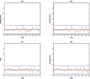
ε are 0.85 and 0.90, respectively. For model (4.2), the first 20 autocorrelations or partial autocorrelations of the residuals _{εˆt} or{εˆ2t}are not significant at the 5% level; see Figure 2. Similar results hold for model (4.3), and hence they are not reported here. Thus, it may imply that both models are adequate to fit _{yt}. Moreover, the values of log-likelihood for models (4.2) and (4.3) are -233.1 and -237.3, respectively, and hence a BAR(2) model is more suitable than TAR(2) model to fit _{yt}.

It is interesting to see that models (4.2) and (4.3) basically tell us different stories. Following Tiao and Tsay (1994), if we treat a negative growth in GNP as ‘contrac-tion’ and a positive growth as ‘expansion’, model (4.2) shows that the region of

0 2 4 6 8 10 12 14 16 18 20 −0.2

0 0.2 0.4 0.6 0.8

Lag

Partial ACF

(a)

0 2 4 6 8 10 12 14 16 18 20 −0.2

0 0.2 0.4 0.6 0.8

Lag

Partial ACF

(b)

0 2 4 6 8 10 12 14 16 18 20 −0.2

0 0.2 0.4 0.6 0.8

Lag

ACF

(c)

0 2 4 6 8 10 12 14 16 18 20 −0.2

0 0.2 0.4 0.6 0.8

Lag

Partial ACF

(d)

Fig 2.(a) the autocorrelations for {εˆt};(b) the partial autocorrelations for{εˆt};(c)the autocor-relations for {εˆ2

t}; and(d)the partial autocorrelations for {εˆ

2

t}.

GNP, and hence the region of yt is most likely unchanged in this case. Thus, based on these facts, it is fair to conclude that a BAR(2) model is more reasonable than TAR(2) model to fit _{yt}.

In the end, it is also of interest to fit_{yt}by a three-regime TAR model as follows:

yt=

                        

−0.4969 + 0.3735yt−1−0.8500yt−2+εtif yt−2 ≤ −0.288

(0.3649) (0.1399) (0.3193)

−3.3614 + 1.1691yt−1−15.872yt−2+εtif−0.288< yt−2 ≤ −0.058

(1.2807) (1.0193) (4.3454)

0.3837 + 0.3233yt−1+ 0.1908yt−2+εt if yt−2 >−0.058

(0.1439) (0.0818) (0.1083)

,

(4.4)

where model (4.4) is estimated by the least squares method with the standard errors in parentheses, and the estimated value ofσ2

compared to model (4.4), we prefer to fit _{yt} by a BAR(2) model in view of this point.

ACKNOWLEDGEMENTS

The authors greatly appreciate the helpful comments of Dr. G.D. Li, two anony-mous referees, the Associate Editor, and the Editor Qiwei Yao. The authors would to thank the Research Grants Council of the Hong Kong SAR Government, GRF grant HKU703711P, for partial support. The first author’s research is also supported by NSFC(No.11201459) and the National Center for Mathematics and Interdisciplinary Sciences, CAS.

REFERENCES

[1] Andrews, D.W.K. (1993a) Tests for parameter instability and structural change with un-know change point.Econometrica61_{, 821-856.}

[2] Andrews, D.W.K.(1993b) An introduction to econometric applications of functional limit theory for dependent random variables.Econometric Reviews 12_{, 183-216.}

[3] Caner, M.andHansen, B.E.(2001) Threshold autoregression with a unit root. Economet-rica69_{, 1555-1596.}

[4] Chan, K.S.(1990) Testing for threshold autoregression.Annals of Statistics 18_{, 1886-1894.}

[5] Chan, K.S. (1991) Percentage points of likelihood ratio tests for threshold autoregression. Journal of the Royal Statistical Society Series B53_{, 691-696.}

[6] Chan, K.S. and Tong, H. (1990) On likelihood ratio tests for threshold autoregression. Journal of the Royal Statistical Society Series B52_{, 469-476.}

[7] Davies, R.B.(1977) Hypothesis testing when a nuisance parameter is present only under the alternative.Biometrica 64_{, 247-254.}

[8] Davies, R.B.(1987) Hypothesis testing when a nuisance parameter is present only under the alternative.Biometrica 74_{, 33-43.}

[9] Doukhan, P.,Massart, P., andRio, E.(1995) Invariance principles for absolutely regular empirical processes.Annales de I’Institut H. Poincare31 _393-427.

[10] Hansen, B.E.(1996) Inference when a nuisance parameter is not indentified under the null hypothesis.Econometrica64_{, 413-430.}

[11] Hansen, B.E.(1999) Threshold effects in non-dynamic panels: Estimation, testing, and in-ference. Journal of Econometrics93_{, 345-368.}

[12] Li, G.D., Guan, B., Li, W.K., andYu, P.L.H. (2012) Buffered threshold autoregressive time series models. Working paper. University of Hong Kong.

[13] Li, G.D. and Li, W.K. (2008) Testing for threshold moving average with conditional het-eroscedasticity.Statistica Sinica18_{, 647-665.}

[14] Li, G.D. and Li, W.K. (2011) Testing a linear time series models against its threshold extension. Biometrika98_{, 243-250.}

[16] Ling, S. and Tong, H. (2005) Testing a linear MA model against threshold MA models. Annals of Statistics33_{, 2529-2552.}

[17] Pham, T.D.andTran, L.T.(1985) Some mixing properties of time series models.Stochastic Processes and their applications19_{, 297-303.}

[18] Potter, S.M.(1995) A nonlinear approach to U.S. GNP.Journal of Applied Econometrics 10_{, 109-125.}

[19] Stute, W. (1997) Nonparametric model checks for regression.Annals of Statistics25_, 613-641.

[20] Tiao, G.C. andTsay, R.S.(1994) Some advances in non-linear and adaptive modelling in time-series. Journal of Forecasting13_{, 109-131.}

[21] Tong, H.(1978) On a threshold model. In Pattern Recognition and Signal Processing (C.H. Chen, ed.) 101-141. Sijthoff and Noordhoff, Amsterdam.

[22] Tong, H. (1990) Non-linear Time Series. A Dynamical System Approach. Clarendon Press, Oxford.

[23] Tong, H. (2011) Threshold models in time series analysis–30 years on (with discussions). Statistics and Its Interface 4_{, 107-135.}

[24] Tsay, R.S.(1989) Testing and modeling threshold autoregressive processes.Journal of Amer-ican Statistical Association 84_{, 231-240.}

[25] Tsay, R.S.(1998) Testing and modeling multivariate threshold models.Journal of American Statistical Association 93_{, 1188-1202.}

[26] Wong, C.S. and Li, W.K. (1997) Testing for threshold autoregression with conditional heteroscedasticity. Biometrika84_{, 407-418.}

[27] Wong, C.S. and Li, W.K. (2000) Testing for double threshold autoregressive conditional heteroscedastic model.Statistica Sinica10_{, 173-189.}

[28] Zhu, K. and Ling, S.(2012) Likelihood ratio tests for the structural change of an AR(p) model to a threshold AR(p) model.Journal of Time Series Analysis33_{, 223-232.}

[29] Zhu, K.,Yu, P.L.H.andLi, W.K.(2013) Testing for the buffered autoregressive processes (Supplementary Material).

Chinese Academy of Sciences Institute of Applied Mathematics HaiDian District, Zhongguancun Bei Jing, China

E-mail:kzhu@amss.ac.cn

Department of Statistics and Actuarial Science University of Hong Kong

Pokfulam Road, Hong Kong E-mail:plhyu@hku.hk

PROCESSES (SUPPLEMENTARY MATERIAL)

By Ke Zhu, Philip L.H. Yu and Wai Keung Li

Chinese Academy of Sciences and University of Hong Kong

APPENDIX: PROOFS

In this appendix, we first give the proofs of Lemmas 2.1-2.2. DenoteC as a generic

constant which may vary from place to place in the rest of this paper. The proofs of Lemmas 2.1-2.2 rely on the following three basic lemmas:

Lemma A.1. Suppose thatytis strictly stationary, ergodic and absolutely regular

with mixing coefficientsβ(m) = O(m−A_{)for someA > v/(v−1)andr > v >1; and}

there exists anA0 >1such that2A0rv/(r−v)< A. Then, for anyγ = (rL, rU)∈Γ,

we have

∞ X

j=1







E





j

Y

i=1

I(rL < yt−i ≤rU)



 





(r−v)/2A0rv

<_∞.

Proof. First, denote ξi = I(rL < yt−i ≤ rU). Then, ξi is strictly stationary,

ergodic and α-mixing with mixing coefficients α(m) = O(m−A_{). Next, take ι ∈}

³

[2A0rv/(r−v) + 1]/(A+ 1),1

´

, and let p=_⌊jι_{⌋ and s =⌊j/j}ι_{⌋, where ⌊x⌋ is the}

largest integer not greater than x. Whenj _≥j0 is large enough, we can always find

{ξkp+1}ks−=01, a subsequence of {ξi}ji=1.

Furthermore, let _Fn

m = σ(ξi, m ≤ i ≤ n). Then, ξkp+1 ∈ Fkpkp+1+2. Note that

E[ξkp+1] < P(a ≤ yt ≤ b) , ρ ∈ (0,1). Hence, by Proposition 2.6 in Fan and

Yao (2003, p.72), we have that for j _≥j0,

E





j

Y

i=1

ξi



≤E

"_s−1 Y

k=0

ξkp+1

#

=

(

E

"_s−1 Y

k=0

ξkp+1

#

− s−1

Y

k=0

E[ξkp+1]

)

+

s−1

Y

k=0

E[ξkp+1]

≤16(s₋1)α(p) +ρs

≤C_⌊j/jι_⌋⌊jι_⌋−A+ρ⌊j/jι ⌋_.

Therefore, since (r₋v)/2A0rv >0, by using the inequality (x+y)k ≤ C(xk+yk)

for any x, y, k > 0, it follows that

∞ X

j=1







E





j

Y

i=1

ξi



 





(r−v)/2A0rv

≤(j0−1) +

∞ X

j=j0







E





j

Y

i=1

ξi



 





(r−v)/2A0rv

≤(j0−1) +C

∞ X

j=j0

h

⌊j/jι_⌋⌊jι_⌋−Ai(r−v)/2A0rv

+C

∞ X

j=j0

ρ⌊j/jι

⌋(r−v)/2A0rv

.

(A.1)

Since ι >[2A0rv/(r−v) + 1]/(A+ 1), we have (ιA+ι−1)(r−v)/2A0rv >1, and

hence P∞

j=1j−(ιA+ι−1)(r−v)/2A 0rv

<_∞, which implies that

∞ X

j=j0

"

⌊j/jι_⌋ ⌊jι_⌋A

#(r−v)/2A0rv ≤

∞ X

j=1

"

j jι_(jι₋₁₎A

#(r−v)/2A0rv

<_∞.

(A.2)

On the other hand, since ³ρ⌊j/jι

⌋(r−v)/2A0rv´1/j

<1, by Cauchy’s root test, we have

∞ X

j=j0

ρ⌊j/jι

⌋(r−v)/2A0rv

<

∞ X

j=1

ρ⌊j/jι

⌋(r−v)/2A0rv

<_∞.

(A.3)

Now, the conclusion follows directly from (A.1)-(A.3). This completes the proof.

Lemma A.2. Suppose that the conditions in Lemma A.1 hold, and yt has a

bounded and continuous density function. Then, there exists a B0 >1 such that for

any γ1, γ2 ∈Γ, we have

kRt(γ1)−Rt(γ2)k2rv/(r−v)≤C|γ1−γ2|(r−v)/2B0rv.

Proof. Let γ1 = (r1L, r1U) and γ2 = (r2L, r2U). Since Rt(γ) = I(yt−d ≤ rL) +

Rt−1(γ)I(rL< yt−d≤rU), we have

Rt(γ1)−Rt(γ2) = ∆t(γ1, γ2) +I(r1L< yt−d≤r1U) [Rt−1(γ1)−Rt−1(γ2)],

where

∆t(γ1, γ2) =I(r2L< yt−d≤r1L)

Thus, by iteration we can show that

Rt(γ1)−Rt(γ2)

= ∆t(γ1, γ2) +

∞ X

j=1

∆t−j(γ1, γ2)

j

Y

i=1

I(r1L < yt−i−d ≤r1U).

(A.4)

Next, for brevity, we assume that r2L ≤ r1L ≤ r2U ≤ r1U, because the proofs for

other cases are similar. Note that for any j _≥0,Rt−j−1(γ2)≤1 and

I(r1L< yt−j−d ≤r1U)−I(r2L < yt−j−d≤r2U)

=I(r2U < yt−j−d≤r1U)−I(r2L< yt−j−d ≤r1L).

Let f(x) be the density function of yt. Since supxf(x) <∞ and |∆t−j(γ1, γ2)| ≤2,

by H¨older’s inequality and Taylor’s expansion, it follows that for any s_≥1,

E_|∆t−j(γ1, γ2)|s≤2s−1E|∆t−j(γ1, γ2)|

≤2s−1

·

2 sup

x f(x)|r1L−r2L|+ supx f(x)|r1U−r2U|

¸

≤C_|γ1−γ2|.

(A.5)

Let A0 >1 be specified in Lemma A.1, and chooseB0 such that 1/A0+ 1/B0 = 1.

By H¨older’s inequality and (A.5), we can show that

E

¯ ¯ ¯ ¯ ¯ ¯

∆t−j(γ1, γ2)

j

Y

i=1

I(r1L < yt−i−d ≤r1U)

¯ ¯ ¯ ¯ ¯ ¯

2rv/(r−v)

≤nE[∆t−j(γ1, γ2)]2B0rv/(r−v)

o1/B0

×







E





j

Y

i=1

I(r1L< yt−i−d≤r1U)



 





1/A0

≤2[2B0rv/(r−v)]−1

{E_|∆t−j(γ1, γ2)|}1/B 0

×







E





j

Y

i=1

I(r1L< yt−i−d≤r1U)



 





1/A0

≤C_|γ1−γ2|1/B0







E





j

Y

i=1

I(r1L< yt−i−d≤r1U)



 





1/A0

.

(A.6)

have

kRt(γ1)−Rt(γ2)k2rv/(r−v)

≤C_|γ1−γ2|(r−v)/2rv +C|γ1 −γ2|(r−v)/2B0rv

×

∞ X

j=1







E





j

Y

i=1

I(r1L< yt−i−d≤r1U)



 





(r−v)/2A0rv

≤C_|γ1−γ2|(r−v)/2B0rv.

This completes the proof.

Lemma A.3. Suppose that the conditions in Lemma A.2 hold and Ey4

t < ∞.

Then,

sup

γ∈Γ

¯ ¯ ¯ ¯ ¯

X′

γX

n −Σγ

¯ ¯ ¯ ¯ ¯

→0 a.s. as n _{→ ∞}.

Proof. For brevity, we only prove the uniform convergence for n−1Pn

t=1φt(γ),

the last component of n−1_X′

γX, where

φt(γ) =y2t−pRt(γ).

First, for fix ε > 0, we partition Γ by _{B1,· · · , BKε}, where Bk = {(rL, rU);ωk <

rL ≤ωk+1, νk < rU ≤νk+1} ∩Γ. Here, {ωk} and {νk} are chosen such that

(ωk+1−ωk)(r−v)/2B

0rv

< C1ε and (νk+1−νk)(r−v)/2B 0rv

< C1ε,

(A.7)

where B0 >1 is specified as in Lemma A.2, and C1 >0 will be selected later.

Next, we set

f_tu(ε) = y_t2_−pRt(ωk+1, νk+1) and ftl(ε) =yt2−pRt(ωk, νk).

By construction, since Rt(γ) is a nondecreasing function with respect to rL and rU,

for any γ _∈Γ, there is some k such that γ _∈Bk and ftl(ε)≤φt(γ)≤ftu(ε).

Furthermore, since rv/(2rv₋r+v)<1, we have

° ° °y

2

t−p

° ° °

2rv/(2rv−r+v)<

° ° °y

2

t−p

° ° °

Thus, by H¨older’s inequality, Lemma A.2 and (A.7), we have

Ehf_tu(ε)₋f_tl(ε)i

≤°° °y

2

t−p

° °

°_{2rv/(2rv−r+v)}kRt(ωk+1, νk+1)−Rt(ωk, νk)k2rv/(r−v)

≤Ch(ωk+1−ωk)(r−v)/2B0rv + (νk+1−νk)(r−v)/2B0rv

i

≤2CC1ε.

By setting C1 = (2C)−1, we have E

h

fu

t(ε)−ftl(ε)

i

≤ε. Thus, the conclusion holds

according to Theorem 2 in Pollard (1984, p.8). This completes the proof.

Proof of Lemma 2.1. First, since Kγγ is positive definite by Assumption 2.1,

we know that both Σ and Σγ are positive definite. By using the same argument

as for Lemma 2.1(iv) in Chan (1990), it is not hard to show that for every γ _∈ Γ,

Σγ−ΣγΣ−1Σ′γ is positive definite. Second, by the ergodic theorem, it is easy to see

that

X′_X

n →Σ a.s. asn → ∞.

(A.8)

Third, by Lemma A.3 we have

sup

γ∈Γ

¯ ¯ ¯ ¯ ¯

X′

γX

n −Σγ

¯ ¯ ¯ ¯

¯→

0 and sup

γ∈Γ

¯ ¯ ¯ ¯ ¯

X′

γXγ

n −Σγ

¯ ¯ ¯ ¯

¯→

0 a.s. (A.9)

as n_{→ ∞}. Note that if H0 holds, we have

Tγ =

1

√

n

n

X_γ′ ₋X_γ′X(X′X)−1X′oε

= √1

n

³

−(Xγ′X)(X′X)−1, I

´

Zγ′ε.

Then, (i) and (ii) follow readily from (A.8)-(A.9). This completes the proof. ¤

Proof of Lemma 2.2. Denote

Gn(γ)≡

1

√

nZ

′

γε=

1

√

n

N

X

t=p

xt(γ)εt.

It is straightforward to show that the finite dimensional distribution of _{Gn(γ)}

converges to that of _{σGγ}. By Pollard (1990, Sec.10), we only need to verify the

4 in Doukhan, Massart, and Rio (1995, p.405); see also Andrews (1993) and Hansen (1996).

First, the envelop function is sup_γ|xt(γ)εt| = ¯xt|εt|, where ¯xt = supγ|xt(γ)|. By

H¨older’s inequality and Assumption 2.1, we know that the envelop function is L2v

bounded. Next, for anyγ1, γ2 ∈Γ, by Assumptions 2.1-2.3, Lemma A.2 and H¨older’s

inequality, we have

kxt(γ1)εt−xt(γ2)εtk2v =kht(γ1)εt−ht(γ2)εtk2v

≤ kxtεtk2rkRt(γ1)−Rt(γ2)k2rv/(r−v) ≤C_kxtk4rkεtk4r|γ1−γ2|(r−v)/2B

0rv

≤C_|γ1−γ2|(r−v)/2B0rv

for some B0 >1, where the last inequality holds since kxtk4rkεtk4r<∞.

Now, following the argument in Hansen (1996, p.426), we know that Gn(γ) is

stochastically equicontinuous. This completes the proof. ¤

Next, we give Lemmas A.4-A.6, in which Lemma A.4 is crucial for proving Lemma A.5, and Lemmas A.5 and A.6 are needed to prove Corollary 2.1 and Theorem 3.1, respectively.

Lemma A.4. Suppose that yt is strictly stationary and ergodic. Then, (i) n0 =

Op(1); (ii) furthermore, if E|yt|2 <∞ and E|εt|2 <∞, for any an=o(1), we have

sup

γ∈Γ

¯ ¯ ¯ ¯ ¯ ¯

an n0−1

X

t=p

xtx′tRt(γ)

¯ ¯ ¯ ¯ ¯ ¯

=Op(1)

(A.10)

and

sup

γ∈Γ

¯ ¯ ¯ ¯ ¯ ¯

an n0−1

X

t=p

ht(γ)εt

¯ ¯ ¯ ¯ ¯ ¯

=Op(1).

(A.11)

Proof. First, by the ergodic theory, we have that

1

M

M

X

t=p

I(a_≤yt−d≤b) =P(a≤yt−d≤b),κ >0 a.s.

as M _{→ ∞}. Thus, _∀η >0, there exists an integer M(η)>0 such that

P





1

M

M

X

t=p

I(a_≤yt−d ≤b)<

κ

2



By the definition of n0, it follows that

P (n0 > M) =P





M

X

t=p

I(a_≤yt−d≤b) = 0

  =P   1 M M X

t=p

I(a_≤yt−d≤b) = 0

  ≤P   1 M M X

t=p

I(a_≤yt−d ≤b)<

κ 2   < η, (A.12)

i.e., (i) holds. Furthermore, by taking ˜M =M2_{, from (A.12) and Markov’s inequality,}

it follows that _∀η >0,

P



sup

γ∈Γ

¯ ¯ ¯ ¯ ¯ ¯ an n0−1

X

t=p

xtx′tRt(γ)

¯ ¯ ¯ ¯ ¯ ¯

>M˜





=P



sup

γ∈Γ

¯ ¯ ¯ ¯ ¯ ¯ an n0−1

X

t=p

xtx′tRt(γ)

¯ ¯ ¯ ¯ ¯ ¯

>M , n˜ 0 ≤M





≤P



 max

p≤k≤Msup_γ∈Γ

¯ ¯ ¯ ¯ ¯ ¯ an k−1

X

t=p

xtx′tRt(γ)

¯ ¯ ¯ ¯ ¯ ¯

>M˜





≤ M

X

k=p

P



a_n

k−1

X

t=p

|xt|2 >M˜





≤an M

X

k=p k−1

X

t=p

E_|xt|2

˜

M

=O

Ã

anM2

˜

M

!

=O(an)< η

(A.13)

as n is large enough. Thus, we know that equation (A.10) holds. Next, by H¨older’s

inequality and a similar argument as for (A.13), it is not hard to show that _∀η >0,

P



sup

γ∈Γ

¯ ¯ ¯ ¯ ¯ ¯ an n0−1

X

t=p

ht(γ)εt

¯ ¯ ¯ ¯ ¯ ¯

>M˜



≤O(a_n)< η

Lemma A.5. If Assumptions 2.1-2.3 hold, then it follows that underH0 or H1n,

(i) sup

γ∈Γ

¯ ¯ ¯ ¯ 1 n ³

Xγ−X˜γ

´′

X

¯ ¯ ¯

¯=op(1),

(ii) sup

γ∈Γ

¯ ¯ ¯ ¯ 1 n ³

X_γ′Xγ−X˜

′

γX˜γ

´¯_¯

¯

¯=op(1),

(iii) sup

γ∈Γ

¯ ¯

¯Tγ−T˜γ ¯ ¯

¯=op(1),

where X˜γ andT˜γ are defined in the same way asXγ and Tγ, respectively, with Rt(γ)

being replaced by R˜t(γ).

Proof. (i) Note that

1

n

³

Xγ−X˜γ

´′

X = _√1

n   1 √ n

n0−1

X

t=p

xtx′tRt(γ)



.

Hence, we know that (i) holds by taking an =n−1/2 in equation (A.10).

(ii) By a similar argument as for (i), we can show that (ii) holds.

(iii) Note that when λ0 = (φ′0, h′/

√

n)′_{, we have}

Tγ−T˜γ =

1

√

n

³

Xγ−X˜γ

´′

ε_−√1 n

³

Xγ−X˜γ

´′

X(X′X)−1X′ε

− 1_n³Xγ−X˜γ

´′

X(X′X)−1X′Xγ0h

− 1_nX˜_γ′X(X′X)−1X′³Xγ0 −X˜γ0

´

h

+ 1

n

³

X_γ′Xγ0 −X˜

′

γX˜γ0

´

h

,I1n(γ)−I2n(γ)−I3n(γ)−I4n(γ) +I5n(γ) say.

First, since

I1n(γ) =

1

n1/4





1

n1/4

n0−1

X

t=p

ht(γ)εt



,

it follows that sup_γ|I1n(γ)|=op(1) by taking an =n−1/4 in equation (A.11). Next,

since

I2n(γ) =





1

n

n0−1

X

t=p

xtx′tRt(γ)



 Ã

X′_X

n

!−1

X′_ε

√

n,

we have that sup_γ|I2n(γ)|=op(1) from (i). Similarly, we can show that supγ|Iin(γ)|=

op(1) fori = 3,4,5. Hence, under H0 (i.e., h≡ 0) or H1n, we know that (iii) holds.

Lemma A.6. If Assumptions 2.1-2.3 hold, then it follows that underH0 or H1n,

sup

γ∈Γ √

n_|λn(γ)−λ0|=Op(1).

Proof. First, for anyγ _∈Γ, by Taylor’s expansion we have

N

X

t=p

h

ε2

t(λn(γ), γ)−ε2t(λ0, γ)

i

=₋(λn(γ)−λ0)′





N

X

t=p

2εt(λ0, γ)xt(γ)





+ (λn(γ)−λ0)′





N

X

t=p

xt(γ)xt(γ)′



(λ_n(γ)−λ₀).

(A.14)

Next, when λ0 = (φ′0, h′/

√

n)′_{, we can show that}

1

√

n

N

X

t=p

εt(λ0, γ)xt(γ) =

1

√

nZ

′

γε+

1

√

n

N

X

t=p

xt(γ)[xt(γ0)−xt(γ)]′λ0

= √1

nZ

′

γε+

1

n

N

X

t=p





xtx′t[Rt(γ0)−Rt(γ)]

xtx′t[Rt(γ)Rt(γ0)−Rt(γ)]



h

,G∗n(γ).

(A.15)

Let λmin(γ) > 0 be the minimum eigenvalue of Kγγ. Then, by equations

(A.14)-(A.15), _∀η >0, there exists a M(η)>0 such that

P

Ã

sup

γ∈Γ √

n_|λn(γ)−λ0|> M

!

=P





√

n_|λn(γ)−λ0|> M,

N

X

t=p

h

ε2_t(λn(γ), γ)−ε2t(λ0, γ)

i

≤0

for some γ _∈Γ)

≤P³√n_|λn(γ)−λ0|> M, −2√n|λn(γ)−λ0||G∗n(γ)|

+n_|λn(γ)−λ0|2[λmin(γ) +op(1)]≤0 for some γ ∈Γ

´

≤P³M < √n_|λn(γ)−λ0| ≤2[λmin(γ) +op(1)]−1|G∗n(γ)|

for some γ _∈Γ)

where the last inequality holds because G∗

n(γ) = Op(1) by Lemma 2.2 and Lemma

A.3. Hence, under H0 (i.e., h≡0) orH1n, our conclusion holds. This completes the

proof.

Proof of Corollary 2.1. The conclusion follows directly from Theorems

2.1-2.2 and Lemma A.5. ¤

Proof of Theorem 3.1. We use the method in the proof of Theorem 2 in

Hansen (1996). Let W denote the set of samples ω for which

lim n→∞ 1 n N X

t=p

sup

γ∈Γ|

xt(γ)|ε2t <∞ a.s.,

(A.16)

lim

n→∞_γ,δsup_∈Γ ¯ ¯ ¯ ¯ ¯ ¯ 1 n N X

t=p

xt(γ)xt(δ)′ε2t −σ2Kγδ

¯ ¯ ¯ ¯ ¯ ¯

→0 a.s.

(A.17)

Since sup_γ∈Γ|xt(γ)| ≤

√

2_|xt| and E|xt|ε2t < ∞ due to Assumption 2.1, by the

ergodic theorem we have

lim n→∞ 1 n N X

t=p

sup

γ∈Γ|

xt(γ)|ε2t ≤_nlim_→∞ √

2

n

N

X

t=p

|xt|ε2t <∞ a.s.,

i.e., (A.16) holds. Furthermore, by Assumptions 2.1-2.3 and a similar argument as for Lemma A.3, it is not hard to see that

lim

n→∞_γ,δsup_∈Γ ¯ ¯ ¯ ¯ ¯ ¯ 1 n N X

t=p

xt(γ)xt(δ)′ε2t −σ2Kγδ

¯ ¯ ¯ ¯ ¯ ¯

→0 a.s.,

i.e., (A.17) holds. Thus,P(W) = 1. Take anyω_∈W. For the remainder of the proof,

all operations are conditionally on ω, and hence all of the randomness appears in

the i.i.d. N(0, 1) variables _{vt}.

Define

Z_n∗(γ) = √1

n

N

X

t=p

xt(γ)εtvt.

By using the same argument as in Hansen (1996, p.426-427), we have

Zn∗(γ)⇒σGγ a.s. as n → ∞.

(A.18)

Note that

sup

γ∈Γ|

ˆ

Zn(γ)−Zn∗(γ)| ≤sup γ∈Γ

¯ ¯ ¯ ¯ ¯ ¯ 1 n N X

t=p

xt(γ)xt(γ)′vt

¯ ¯ ¯ ¯ ¯ ¯ sup

γ∈Γ

¯ ¯ ¯

√

n(λn(γ)−λ0)

Using the same argument as for (A.18) (see, e.g., Hansen (1996, p.427)), we have

1

n

N

X

t=p

xt(γ)xt(γ)′vt ⇒0 a.s. asn → ∞.

(A.19)

Now, by Lemma A.6 and (A.19), it follows that under H0 or H1n,

ˆ

Zn(γ)−Zn∗(γ)⇒0 in probability as n→ ∞.

(A.20)

Thus, by (A.18) and (A.20), we know that under H0 or H1n,

ˆ

Zn(γ)⇒σGγ in probability as n→ ∞.

(A.21)

Next, we consider the functional

L:x(_·)_∈D2p+2(Γ)→

1

σ2 sup

γ∈Γ

x(γ)′Ωγx(γ),

where D2p+2(Γ) denotes the function spaces of all functions, mapping R2(Γ) into

R2p+2_{, that are right continuous and have right-hand limits. Clearly, L(·) is a}

con-tinuous functional; see e.g., Chan (1990, p.1891). By the concon-tinuous mapping theory

and (A.21), it follows that under H0 orH1n,

L( ˆZn(γ))⇒L(σGγ) in probability asn → ∞.

(A.22)

Furthermore, since σ2

n → σ2 a.s. and (X1n(γ), I)′[X2n(γ)]−1(X1n(γ), I) → Ωγ

uni-formly in γ by Lemma A.3, we have that

sup

γ∈Γ

ˆ

LRn(γ) =L( ˆZn(γ)) +op(1).

(A.23)

Finally, the conclusion follows from (A.22)-(A.23). This completes the proof. ¤

Proof of Corollary 3.1. Conditional on the sample _{y0,· · · , yN}, let ˆFn,J

and ˆFn be the conditional empirical c.d.f. and c.d.f. of ˆLRn, respectively. Then,

P ³LRn ≥cJn,α

´

=EhP ³LRn≥cJn,α|y0,· · · , yN

´i

=EhP ³Fˆn,J(LRn)≥1−α|y0,· · · , yN

´i

By the Glivenko-Cantelli Theorem and Theorem 3.1, it follows that under H0 or

H1n,

lim

n→∞Jlim→∞P ³

LRn ≥cJn,α

´

= lim

n→∞E h

P³Fˆn(LRn)≥1−α|y0,· · · , yN

´i

= lim

n→∞E[P(F0(LRn)≥1−α|y0,· · · , yN)]

= lim

n→∞P(F0(LRn)≥1−α),

(A.24)

where F0 is the c.d.f. of supγ∈ΓG′γΩγGγ. Thus, by (A.24) and Theorem 2.1, under

H0 we have

lim

n→∞Jlim→∞P ³

LRn ≥cJn,α

´

=P

Ã

sup

γ∈Γ

G′_γΩγGγ ≥F0−1(1−α)

!

=α,

i.e., (i) holds. Furthermore, by (A.24) and Theorem 2.2, under H1n we have

lim

h→∞nlim→∞Jlim→∞P ³

LRn≥cJn,α

´

= lim

h→∞P ³

Bh ≥F0−1(1−α)

´

= 1,

whereBh ,supγ∈Γ

n

G′

γΩγGγ+h′µγγ0h

o

and the last equation holds since Bh → ∞

in probability as h_{→ ∞}. Thus, (ii) holds. This completes the proof. ¤

REFERENCES

[1] Andrews, D.W.K. (1993) An introduction to econometric applications of functional limit

theory for dependent random variables.Econometric Reviews 12_{, 183-216.}

[2] Chan, K.S.(1990) Testing for threshold autoregression.Annals of Statistics 18_{, 1886-1894.}

[3] Doukhan, P.,Massart, P., andRio, E.(1995) Invariance principles for absolutely regular

empirical processes.Annales de I’Institut H. Poincare31 _393-427.

[4] Fan, J.andYao, Q.(2003) Nonlinear time series: Nonparametric and parametric methods. Springer, New York.

[5] Hansen, B.E.(1996) Inference when a nuisance parameter is not indentified under the null

hypothesis.Econometrica64_{, 413-430.}

[6] Pollard, D.(1984) Convergence of Stochastic Processes. New York: Springer.

[7] Pollard, D. (1990) Empirical processes: Theory and applications. NSF-CMBS Regional Conference Series in Probability and Statistics, Vol 2. Hayward, CA: Institute of Mathematical Statistics.

Chinese Academy of Sciences Institute of Applied Mathematics HaiDian District, Zhongguancun Bei Jing, China

E-mail:zkxaa@ust.hk

Department of Statistics and Actuarial Science University of Hong Kong

Pokfulam Road, Hong Kong

E-mail:plhyu@hku.hk