Munich Personal RePEc Archive
A comparison of public and private
schools in Spain using robust
nonparametric frontier methods
Cordero, José Manuel and Prior, Diego and Simancas
Rodríguez, Rosa
University of Extremadura, Autonumous University of Barcelona,
University of Extremadura
November 2013
Online at
https://mpra.ub.uni-muenchen.de/51375/
“A comparison of public and private schools in Spain using robust
nonparametric frontier methods”
José Manuel Cordero University of Extremadura
Diego Prior
Autonomous University of Barcelona ([email protected])
Rosa Simancas University of Extremadura
Abstract
This paper uses an innovative approach to evaluate educational performance of Spanish students in PISA 2009. Our purpose is to decompose their overall inefficiency between different components with a special focus on studying the differences between public and state subsidized private schools. We use a technique inspired by the non-parametric Free Disposal Hull (FDH) and the application of robust order-m models, which allow us to mitigate the influence of outliers and the curse of dimensionality. Subsequently, we adopt a metafrontier framework to assess each student relative to the own group best practice frontier (students in the same school) and to different frontiers constructed from the best practices of different types of schools. The results show that state-subsidised private schools outperform public schools, although the differences between them are significantly reduced once we control for the type of students enrolled in both type of centres.
Key words: Education, Efficiency, Multilevel Modelling, Free Disposal Hull.
1. INTRODUCTION
Since the pioneer study of Coleman et al. (1982), the debate about the performance of private
and public schools has become one of the main topics of research in a wide range of educational
contexts (Rouse and Barrow, 2009). In general terms, it is widely assumed that private schools
are likely to perform better than public schools because market competition forces them to
achieve a more efficient use of resources (Friedman and Friedman, 1981; Chubb and Moe,
1990; Hoxby 2003). However, empirical studies comparing both, public and private schools,
need to control for differences in the personal and socio-economic background of students as
well as the potential self-selection bias that can arise because more informed and motivated
parents are more likely to apply to better schools (Mayston, 2003; Tamm, 2008; Burgess and
Briggs, 2010).
The conclusions reached in the vast literature devoted to this issue are mixed. Some studies find
that private schools do better, even after controlling for the aforementioned factors (Jiménez et
al., 1991; Toma, 1996; Altonji et al., 2005; Dronkers and Roberts, 2008; Annand et al., 2009;
Dronkers and Avram, 2010; Kim, 2011), although those differences are reduced or disappear
when those variables are taken into account (Williams and Carpenter, 1991; Goldhaber, 1996;
Sander, 1996; McEwan and Carnoy, 2000; McEwan, 2001; Hsieh and Urquiola, 2006; Chudgar
and Quin, 2012) or even public schools can outperform private ones (Bifulco and Ladd, 2006;
Newhouse and Beegle, 2006).
This paper contributes to the above literature by applying a new method to estimate the
differences in efficiency between public and private schools. In this sense, it must be noted that
the educational system in Spain represents a relevant case study, since two types of schools
compete for public funds: public and state-subsidized private schools1. The former are managed
by public authorities while the latter are owned and managed directly or indirectly by a private
non-government organization (mainly Catholic entities)2. This scheme aims at allowing parents
to freely design their preferred school and, indirectly, stimulating competition among schools to
1
There are also private government-independent schools, controlled by non-government organizations, which are mainly funded through student fees. However, in this paper, we focus only on the publicly financed schools.
2
improve their performance. In this context, the comparison between their levels of efficiency
becomes extremely attractive.
In fact, the recent literature provides some empirical studies focused on this comparison using
Spanish data with different methodological approaches, although the findings are still
inconclusive. Hence, Mancebon and Muñiz (2008) do not find significant differences after using
an extension of Silva Portela and Thanassoulis (2001) proposal. The same conclusion is reached
by Calero and Escardibul (2007) using multilevel analysis and Perelman and Santin (2011)
using parametric stochastic distance functions. Mancebon et al. (2012) obtain even better results
for public schools combining the use of multilevel analysis with the same extension of DEA. In
contrast, Crespo et al. (2013) conclude that, after applying a propensity score matching
technique to correct the potential bias, students attending state-subsidized private schools
perform significantly better than students from public schools.
In this paper, we combine the application of two recently developed nonparametric methods to
estimate the efficiency of both types of schools. Firstly, we use the order-m partial frontiers
approach (Cazals et al., 2002) in order to avoid some of the main drawbacks of the
nonparametric methods, such as the high impact of atypical observations or the bias that can
arise when the evaluated units (students) are grouped into groups (schools) of different size
(Zhang and Bartels, 1998). This approach consists of using only part of the sample (m
observations) to determine efficiency scores, thus it mitigates the impact of outliers and
potential errors in data and assures the same size for the reference set, avoiding the curse of
dimensionality that systematically pursues the traditional nonparametric estimations (Daraio and
Simar, 2007). Secondly, in order to assess the performance of both types of schools we adopt
the metafrontier framework, developed by Battese and Rao (2002), Battese et al. (2004) and
O´Donnell et al. (2008). This method allows us to assess each student relative to their own
group (meaning, students attending the same type of schools) and, secondly, to the overall
metafrontier, constructed from the best practices of both types of schools.
De Witte et al. (2010) were pioneers in using those methods to assess the performance of a
sample of British secondary schools, although they only evaluate public centres. Cherchye et al.
(2010) also used a robust nonparametric approach to assess educational efficiency of Flemish
pupils attending public and private primary schools, although their comparison between
different types of schools is based on stochastic dominance criteria. De Witte and Kortelainen
(2013) use the partial order-m approach to estimate the efficiency of Dutch pupils in PISA, but
students and not on comparing public and private schools. Finally, Thieme et al. (2013)
represents the only previous study in which both approaches employed in this paper are
combined to assess the performance of students in primary education in Chile, although they do
not consider the managerial decomposition between public and private schools. Therefore, this
paper represents the first combined application of both methods using data from secondary
schools. In particular, we analyse the performance of Spanish students in PISA 2009, which
provides a wide volume of data regarding multiple factors that can affect the performance at
student and school level.
One of the main advantages of this paper is the possibility of working with student level data,
which facilitates the interpretation of the results and assist in the estimation of the multiple
factors affecting the performance of students (Summers and Wolf, 1977; Hanushek et al., 1996).
Furthermore, the measurement of efficiency at student level allows considering separately
student’s own socioeconomic background and their schoolmates´ one (the so-called peer-group
effect), two inputs which cannot be simultaneously included with aggregated data (Santín,
2006).
The rest of the paper is organized as follows. Section 2 presents the methods used to estimate
students´ efficiency and separate the school effect. Section 3 describes the main characteristics
of the dataset and the criteria followed to select the variables included in the analysis. Section 4
discusses the main results. Finally, section 5 provides concluding remarks.
2. METHODOLOGY
2.1. The deterministic model
The definition of the production technology that a student uses to acquire knowledge is a very
difficult task. The only thing that we know is that pupils transform a set of inputs
)
(
qx
x
∈
ℜ
+ such as their own capabilities or their parental background into heterogeneousoutputs
y
(
y
∈
ℜ
q+)
, usually represented by their results in standardized test scores. This can berepresented by equation (1):
{
p qy
x
∈
ℜ
++=
(
,
)
Given that the production set cannot be observed, some assumptions are required such as the
free disposability of inputs and outputs and the feasibility of all the combinations of those
variables. In order to estimate the relative efficiency of each student, we need to constitute a
frontier that represents the best performing students. This boundary set is characterized by the
following expression:
}
{
(
,
)
∈
(
,
)
∉
,
∀
0
<
<
1
,
(
,
)
∉
,
∀
>
1
=
ψ
θ
ψ
θ
λ
ψ
λ
θψ
x
y
x
y
x
y
(2)According to this definition, the efficient students will be part of the frontier, while the
inefficiency of those that do not belong to the frontier can be measured using equation (3) for
input orientation or equation (4) for output orientation. However, in this paper we will focus on
the latter option, since in the educational context the goal of the pupil is to achieve the best
feasible results.
{
θ
θ
ψ
}
θ
(
x
,
y
)
=
inf
(
x
,
y
)
∈
(3){
λ
λ
ψ
}
θ
(
x
,
y
)
=
sup
(
x
,
y
)
∈
(4)A procedure to measure the relative inefficiency scores θ and λ is represented by nonparametric
techniques, represented by Data Envelopment Analysis –DEA– (Charnes et al., 1978) and Free
Disposal Hull –FDH– (Deprins et al., 1984). This approach is based on mathematical
programming and does not require the imposition of a determined form on the production
function. Both DEA and FDH estimate the technology set ψ by the smallest set
ψ
ˆ
that envelopsthe observed data, but FDH differs from DEA in its removal of the convexity assumption:
}
{
x
y
p qy
y
ix
x
ii
n
FDH
(
,
)
;
;
1
,....,
ˆ
=
∈
ℜ
++≤
≥
=
ψ
(5)In practical terms, this implies that each unit (student) is compared only to other existing unit
(student), and that it cannot be evaluated against any convex combinations of efficient units. As
a result, the FDH frontier can be considered even more flexible than DEA, since there are even
fewer required assumptions.
Although DEA is more popular among researchers in the field of education, in our study we opt
for using FDH because it has higher flexibility, it has comparatively superior asymptotic
real3. The output oriented efficiency score (
θ
ˆFDH ) of an observation can be obtained by solvingthe mixed integer linear programming problem in equation (6):
{ }
=
∈
=
≥
≤
=
∑
∑
∑
= = = N i N i N i i i i i i iFDH
y
y
x
x
i
n
1 1 1
,....,
1
;
1
,
0
;
1
;
;
max
ˆ
λ
λ
γ
γ
γ
γ
θ
(6)where
θ
ˆFDH =1 denotes an efficient pupil, whileθ
ˆFDH >1implies that the pupil is inefficient.However, this nonparametric approach, as well as DEA, presents some significant shortcomings
that should be born in mind when using nonparametric methods to assess efficiency at student
level: (1) statistical inference is not possible due to its deterministic nature; (2) it is very
sensitive to the presence of outliers and measurement errors in data; (3) it experiences
dimensionality problems due to their slow convergence rates. In the next sections, we explain
some approaches that can be used in order to overcome these limitations.
2.2. The robust approach
The first attempts to improve the robustness of nonparametric methods were the works of
Kneipp et al. (1998) and Simar and Wilson (2000). Subsequently, Cazals et al. (2002)
introduced the robust order-m estimation. This approach is related to the FDH estimator, but
instead of constructing a full frontier, it creates a partial frontier that envelops only m (≥1)
observations randomly drawn from the sample. This procedure is repeated B times resulting in
multiple measures (
θ
ˆ
mi1,...,
θ
ˆ
miB ) from which the final order-m efficiency measure is computed asthe simple mean (
θ
ˆ
mi). Specifically, the order-m efficiency score is derived from equation (7):
≥
=
= =y
y
x
x
E
j ij i p j m i
m
min
1,..,max
1,..,θ
(7)where the ρ-dimensional random variables xi,…,xm are drawn randomly and repeatedly from the
conditional distribution of X given yi ≥ y. This estimator allows us to compare the efficiency of
an observation with that of m potential units that have a production larger or equal to y. As it
does not include all the observations, it is less sensitive to outliers, extreme values or noise in
3
the data. As m increases, the expected order-m estimator tends to the FDH efficiency score
(
θ
ˆFDH ). For acceptable m values, normally the efficiency scores will present values higher thanunity, which indicates that students are inefficient, as outputs can be increased without
modifying the level of inputs. When
θ
ˆ
<
1
, the student can be labelled as super-efficient, since the order-m frontier exhibits lower levels of outputs than the student under analysis. This is notpossible in the traditional nonparametric framework where by construction
θ
ˆ
≥
1
.Moreover, this approach allows us to avoid the problem of bias that can arise when we compare
groups of units on a different size, which is the case in our application with schools, since the
mean level of efficiency generally depends on the existing observations in each school (Zhang
and Bartels, 1998). This problem can be reduced by using the same m parameter for every
school, which implies assuming that the performance of every student is compared to the same
number of students independently of the number of students in his/her school. In our case, we
determine the value of m that equals the size of the smallest school in the data set (20), since it
fits better in the metafrontier framework (see below). The main advantage of a lower trimming
value m is the reduced sensibility to outlying observations in the sample, although it also
implies that the probability of drawing the evaluated observation is rather low and,
consequently, we will observe more super-efficient observations.
2.3. The metafrontier approach
Independently of the method employed to estimate the efficiency coefficients, we need to bear
in mind that part of those estimates derives from the environmental situation of the school they
attend. Therefore, results obtained with frontier models need to control for this heterogeneity in
order to give significance to the results.
For that purpose, we adapt the metafrontier approach developed by Battese and Rao (2002),
Battese et al. (2004) and O`Donnell et al. (2008) to deal with a hierarchical structure in data,
which is typical in the educational context, where students (level 1) are nested within schools
(level 2). This approach measures the efficiency of units relative to separate best practice
frontiers and allows us to decompose the performance of each student into a part attributable to
the school and a part attributable to his/her skills. If there are K schools, each having their own
technology and environmental factors, a metafrontier is defined as the boundary of the
frontiers. Separetely, the local efficiency of the student with regards to the type of school he is
involved in is measured relative to the nkobservations in the school sample:
{
k}
k k k k k
k k
y x y
x
θ
θ
ψ
θ
( , )=inf ( , )∈ (8)where the technology set for group k is defined as
{
p qk k k
y
x
∈
ℜ
++=
(
,
)
ψ
xkcan produce yk}
(9)If all the schools have potential access to the same environment, all the observations can be
pooled and students can be evaluated relative to the same standards. Thus, the metafrontier can
be represented by the technology set defined by:
{
p qy
x
∈
ℜ
++=
(
,
)
ψ
x can produce y}
(10)This approach is basically an extension of the proposal by Silva Portela and Thanassoulis
(2001) and Thanassoulis and Silva Portela (2002) to decompose the effect of school from
students´ inefficiency as well as to distinguish between the types of funding regime under which
the school operates. Given the purpose of this paper, we are more interested in the latter issue,
although we will take into account both aspects in the metafrontier framework. Thus, in a first
step two different types of frontiers are defined: the local frontier specific for each school,
which can be interpreted as the student-within-school efficiency and the overall frontier, which
represents the student-within-all-schools efficiency. According to this definition, the distance to
the local frontier depends only on the student´s efficiency (STE) whereas the distance separating
the local and the overall frontier can be interpreted as the school efficiency (SCE). This can be
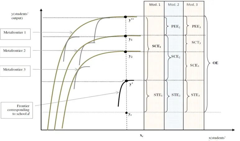
illustrated in Figure 1, where the efficiency level of a student c depends on the level of the
output achieved (yc) using his input endowment (xc). This student is inefficient, since there are
students in the same school obtaining better results (y´) with the same amount of inputs (xc). The
student effect can be defined by the ratio between the local potential output divided by the
actual output (STE = α´= y´/yc). When this student is compared with the metafrontier, the overall
efficiency can be defined as OE = α´´= y´´/yc. From those two measures of efficiency, the school
effect can be automatically derived as SCE1 = y´´/y´= OE/STE. In summary, the global
efficiency can be decomposed in two effects: OE = STE1 x SCE1 (model 1) (Thanassoulis and
However, in order to represent adequately the heterogeneity that exists in each school, the
metafrontier needs to consider not only student data, but also additional variables representing
the characteristics of students attending each school (Thieme et al., 2013). If we do not consider
these variables, we are implicitly assuming that all the schools are operating with the most
favourable environment, which would not be real in many cases. Therefore, it is possible to
improve the definition of the school effect (SCE2 = y1/y´≥1)by considering additional variables.
In particular, we incorporate information about an additional variable: the socioeconomic status
of students enrolled in the same school, i.e., the so-called peer effect4.
The consideration of this variable is based on the assumption that the composition of schools
and classrooms is not random, since it typically reflects neighbourhood characteristics and
therefore the family background of students. The existing literature has used a wide variety of
approaches to identify the peer effect (Mc Ewan, 2003; Lefgren, 2004; Lavy et al., 2012), which
is usually identified by some variable related to student’s classmates. However, we construct a
variable based on the average of the schoolmates´ socioeconomic characteristics due to the lack
of data at class level in the PISA dataset.
Specifically, we have estimated a new model (model 2) that allows us to expand the
decomposition of the overall efficiency:. OE = STE2 x SCE2 x PEE2, where the peer effect can
be defined as PEE = α1= y``/y1. This decomposition is represented in Figure 2, where the
metafrontier 2 considers the characteristics of students corresponding to the school under
analysis, while metafrontier 1 assumes that the school has the optimal level of environmental
factors.
Finally, as we are interested in the effect of the school type (public and private), the
metafrontier needs to be separated between the two types. Silva Portela and Thanassoulis
(2001), based on the previous work of Charnes et al. (1981) to decompose the overall
efficiency, defined two components: managerial and programme inefficiency. Thus, this
approach allows us to distinguish between inefficiency attributable to the institutional
characteristics of the school where the students are enrolled and those attributable to the
management regime under which it is operating. Indeed, the different formal rules Spanish
public and private schools are subject to may influence their relative performance. As an
example, let us pay attention on how it is regulated the teachers’ contracts. On the one hand, in
4
the public schools the director has no capacity to decide which profile of teachers should be
hired (civil servants have stable position and short term contracts are offered to other teachers
without considering the directors’ opinion). On the other, state-subsidized private schools have
more flexibility, since the director can manage the process to hire new teachers. Although it is
not granted in advance, directors of private schools can take advantage of this flexibility and
configure a more homogeneous and focused staff what, finally, can improve the school’s
performance. Nevertheless, public schools traditionally have more qualified teachers with better
pedagogical skills and more experience, although the lack of positive incentives can influence
their behavior and reduce the enthusiasm. An additional factor, coming from the human
resources literature but very important in the education sector, is that the long term horizon in
public schools can influence a positive compromise of the teachers with the strategic goals of
the school (López-Torres and Prior, 2013). Summing up, the question on how interferes the
institutional form of the school on the levels of its efficiency has not an obvious answer, as
competing forces can play a role to modify the net effect.
In order to estimate this new frontier (metafrontier 3), we need to divide the whole sample of
schools into two different subsamples, thus students are only compared among others attending
the same type of school (public or private). Therefore, the previous school effect is decomposed
into two different effects: the type of school (SCT3= α2= y1/y2) and the new school effect (SCE3
= y2/y´≥1) (Figure 3). Once we have defined these new components of the overall inefficiency,
it is straightforward to decompose it between the student effect, the type of school effect, the net
school effect and the peer effect: OE = STE3 x SCT3 x SCE3 x PEE3 (model 3).
3. DATA AND VARIABLES
In this study we assess the performance of Spanish students in PISA (Program for International
Student Assessment) data set in 2009. This sample comprises more than 25,000 students who
are enrolled in almost 900 schools, among which we can distinguish three different typologies:
public, state-subsidized private and pure private schools. As we are only interested in comparing
the performance of schools with a public funding, we excluded totally private schools from the
sample5. Likewise, we also removed schools were the number of available observations did not
reach a minimum number of students (20). As a result, our sample consists of 22,317 students
belonging to 737 schools, among which two thirds are public and one third are state-subsidized
5
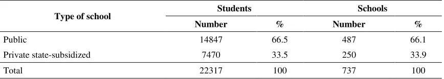
schools (33%). Table 1 provides information on both students and schools included in the
[image:12.595.96.530.165.243.2]sample.
Table 1. Number of students and schools in the sample
With regard to the selection of variables, we follow the same approach used in Mancebon and
Muñiz (2008), where a restrictive efficiency notion is estimated taking into account the
relationship between the academic results obtained by students and their socio-economic
background, since this indicator fulfils the requirements of being continuous and have high
positive correlation with outcome variables (e.g. Coleman et al., 1966; Goldhaber and Brewer,
1997; Hanushek, 2003). According to this criterion, we evaluate whether the student is making
the most of their potential ability, using his/her socioeconomic background as a proxy for this
concept, or his/her performance is below the expected level, i.e., the student-within-school
inefficiency.
The results obtained by students in the three competences evaluated in PISA, mathematics,
reading comprehension and sciences are used as output indicators. These results are not
expressed by only one value, but by five denominated plausible values randomly obtained from
the distribution function of test results derived from the answers in each test (Rasch 1960,
1980), which can be interpreted as the representation of the ability range for each student
(Mislevy et al., 1992; Wu and Adams, 2002). Although PISA analysts recommend to use all of
them to obtain more consistent estimations, in our analysis we use the mean value of those five
plausible values, since the robustness of results is guaranteed by the use of the order-
m
approach, which reduces the impact of measurement error by drawing repeatedly (B
times) observations from the sample.
The input is measured by students’ socioeconomic background (ESCS), an index of economic,
social and cultural status of students created by
PISA analysts that captures a range of
aspects of a student’s family and home background that combines information on
parents’ education and occupations and home possessions. The first variable is the
higher educational level of any of the student’s parents according to the
InternationalType of school Students Schools
Number % Number %
Standard Classification of Education (ISCED, OECD, 1999). The second variable is the highest
labour occupation of any of the student’s parents according to the International Socio-economic
Index of Occupational Status (ISEI, Ganzeboom et al., 1992). The third variable is an index of
educational possessions related to household economy. Given that this continuous indicator
presented negative values6, the original values have been rescaled. As a result, the variable
fulfils the requirement of isotonicity (i.e., ceteris paribus, more input implies equal or higher
level of output) preserving the desirable property of translation invariance (Cooper, Seiford and
Tone, 2007).
Finally, we have selected a variable to include information about the characteristics of students
in each school. This variable is represented by schoolmates’ background, i.e., the so-called
peer-group effect (Patrinos, 1995). It is defined as the average level in the variable ESCS of
students from the same school, whose theoretical ground lies in the fact that the level of
knowledge that can be achieved by a student depends directly on the characteristics of his/her
schoolmates.
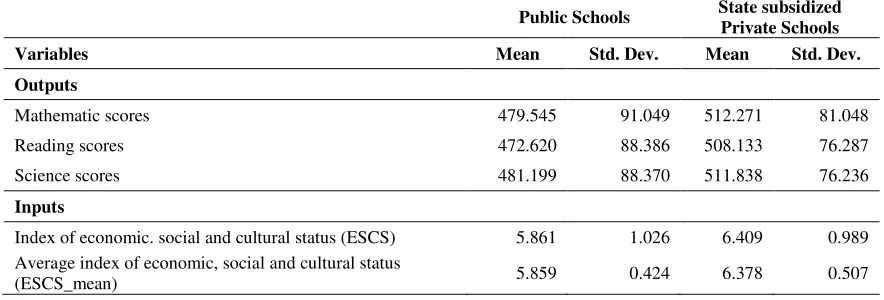
Table 2 reports a comparison between the values of public and private state-subsidized schools
in the four selected variables at student level (three outpus and one input) as well as the
indicator representing the type of students in each school. We can observe that private schools
obtain higher values in all the outcome variables. However those differences can be explained
by the “higher quality” of pupils attending each type of school, represented by their socio
[image:13.595.92.534.543.693.2]economic index.
Table 2. Descriptive statistics of variables included in the analysis
Public Schools State subsidized Private Schools
Variables Mean Std. Dev. Mean Std. Dev.
Outputs
Mathematic scores 479.545 91.049 512.271 81.048 Reading scores 472.620 88.386 508.133 76.287 Science scores 481.199 88.370 511.838 76.236 Inputs
Index of economic. social and cultural status (ESCS) 5.861 1.026 6.409 0.989 Average index of economic, social and cultural status
(ESCS_mean) 5.859 0.424 6.378 0.507
6
4. RESULTS
In this section we present the results obtained using the robust order-m approach to estimate the
efficiency levels (
θ
ˆ
mi) in the three models. First, we estimate model 1, which only allows us toseparate the school effect from overall efficiency calculated for each student. Secondly, we
estimate two different metafrontiers in order to isolate the school effect from other components
of inefficiency. Thus, model 2 determines the importance of the peer effect and how this can
reduce the school effect and, subsequently, in model 3 we consider the different institutional
rules affecting public and private schools. Therefore, in model 3 the school effect will appear as
a residual, after isolating the impact of the peers and the institutional effects.
In our analysis, we use an output orientation, since both the individual students and the schools
are attempting to maximize their attainment. As we mentioned previously, we select the value
20 for the m parameter and we use 200 bootstrap iterations (B) for statistical inference. The
estimation of metafrontiers 1 and 2 uses the whole sample, while the estimation of metafrontier
requires the division of the sample between public and state subsized private schools. Finally,
the decomposition of inefficiency between different effects (STE, SCE, SCT and PEE) requires
the estimation of one partial frontier for each of 737 schools.
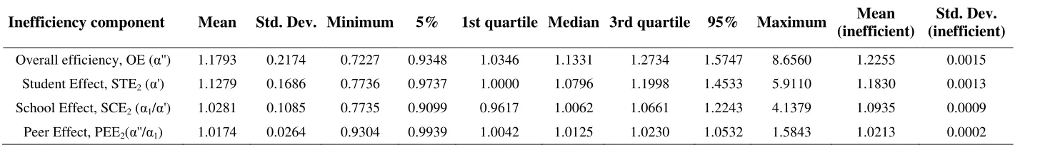
Table 3 reports the summary statistics of the estimated scores for model 1 in all the schools. The
overall efficiency (α´´) for each student in the sample has a mean value of 1.1793, which
indicates that if all students would perform as efficiently as the best practice students, the test
scores could increase on average by 18%7. It must be pointed out that, according to model 1,
most of the inefficiency found is attributable to the student effect (1.1279 on average),
substantially higher than the school effect (1.0461 on average). Moreover, it is worth noting that
some pupils have a performance score below 1. These super-efficient students are performing
better than the average of the (m = 20) students they are benchmarked with. According to the
data shown in Table 4, we can observe that there are significant divergences between public
(1.2017) and private centres (1.1350). The level of inefficiency attributable to the student is
similar in both types of centres, which means that most part of the differences on the overall
inefficiency depends on the school effect. According to the structure of model 1, the effect
attributable to the schools is obtained by dividing the overall efficiency score (α'') by the student
effect (α'). Table 3 indicates that the mean value of this effect is 4.6%, although behind these
7
values it is possible to detect that public schools are more inefficient than private schools
(5.87% vs. 2.11% in Table 4). Those differences are significant according to the value of the
Mann-Whitney nonparametric test applied to these values.
Regarding this point, the results obtained for model 2 are especially informative, because they
allow us to distinguish which part of the school inefficiency can be explained by the
socioeconomic characteristics of peers attending the same school. The results reported in Table
5 show that the importance of this factor is not too relevant if we consider the whole sample;
however, the comparison between public and private schools (Table 6) alert us about the
importance of this factor to explain the inefficiency of students attending public centres
(3.63%), since it represents more than 60% of the initial average score attributed to the school
effect (5.87%). In contrast, this factor has a residual impact on private schools (0.09%), since
most of them are actually facing a favourable environment as we were assuming in model 1.
Moreover, in public schools there is also a significant part of the inefficiency that depends on
the school the student is enrolled (2.16%), while this component has a lower impact in private
schools (1.27%).
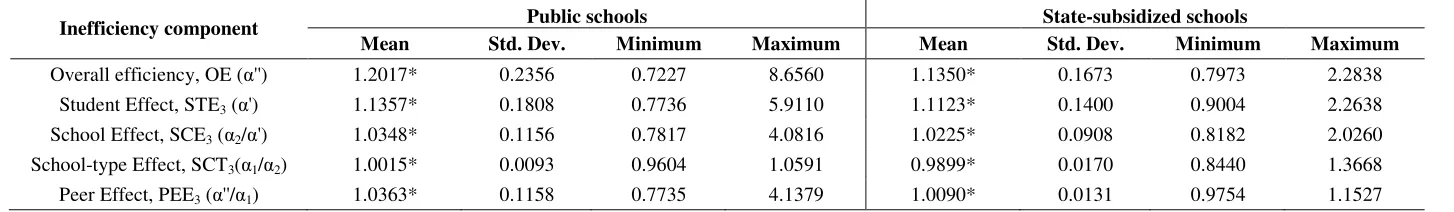
Finally, the values of the school type effect calculated in model 3 have a mean value very close
to 1, with a very low standard deviation for the whole sample (Table 7). This evidence shows
that, once we have taken into account the type of students attending to each type of schools, the
effect attributable to the type of school on inefficiency is almost inexistent (0.997). Therefore,
the remaining divergences in terms of inefficiency depend on the residual factor, i.e., those
variables representing the characteristics of schools that have not been included in the analysis
(school effect).
Although the importance of the school type effect is low, the comparison between public and
state subsidized private schools (Table 8) allows us to identify that the average score assigned to
this effect is lower in private schools than in public schools, which indicates that the former
(where the average level of the variable ESCS is higher) outperform the latter. This evidence is
confirmed by the existence of significant differences in the mean values corresponding to the
two subsamples8.
8
Table 3. Decomposition of overall efficiency between student and school effect (Model 1)
Inefficiency component Mean Std. Dev. Minimum 5% 1st quartile Median 3rd quartile 95% Maximum Mean (inefficient)
Std. Dev. (inefficient)
Overall efficiency, OE (α'') 1.1793 0.2174 0.7227 0.9348 1.0346 1.1331 1.2734 1.5747 8.6560 1.2255 0.0015 Student Effect, STE1 (α') 1.1279 0.1686 0.7736 0.9737 1.0000 1.0796 1.1998 1.4533 5.9110 1.2310 0.0017
[image:16.842.51.772.246.327.2]School Effect, SCE1 (α''/α') 1.0461 0.1136 0.7833 0.9207 0.9759 1.0228 1.0871 1.2499 4.0391 1.2390 0.0019
Table 4. Decomposition of overall efficiency between student and school effect by type of school (Model 1)
Inefficiency component Public schools State-subsidized schools
Mean Std. Dev. Minimum Maximum Mean Std. Dev. Minimum Maximum
Overall efficiency, OE (α'') 1.2017* 0.2356 0.7227 8.6560 1.1350* 0.1673 0.7973 2.2838 Student Effect, STE1 (α') 1.1357* 0.1808 0.7736 5.9110 1.1123* 0.1400 0.9004 2.2638
School Effect, SCE1 (α''/α') 1.0587* 0.1214 0.7833 4.0391 1.0211* 0.0913 0.7972 1.9784
*Test statistics significant at 1% level. (non-parametric Mann–Whitney test)
Table 5. Decomposition of overall efficiency between student, peer and school effect (Model 2)
Inefficiency component Mean Std. Dev. Minimum 5% 1st quartile Median 3rd quartile 95% Maximum Mean (inefficient)
Std. Dev. (inefficient)
Overall efficiency, OE (α'') 1.1793 0.2174 0.7227 0.9348 1.0346 1.1331 1.2734 1.5747 8.6560 1.2255 0.0015 Student Effect, STE2 (α') 1.1279 0.1686 0.7736 0.9737 1.0000 1.0796 1.1998 1.4533 5.9110 1.1830 0.0013
School Effect, SCE2 (α1/α') 1.0281 0.1085 0.7735 0.9099 0.9617 1.0062 1.0661 1.2243 4.1379 1.0935 0.0009
[image:16.842.51.793.371.473.2]Table 6. Decomposition of overall efficiency between student, school-type and school effect by type of school (Model 2)
Inefficiency component Public schools State-subsidised schools
Mean Std. Dev. Minimum Maximum Mean Std. Dev. Minimum Maximum
Overall efficiency, OE (α'') 1.2017* 0.2356 0.7227 8.6560 1.1350* 0.1673 0.7973 2.2838 Student Effect, STE2 (α') 1.1357* 0.1808 0.7736 5.9110 1.1123* 0.1400 0.9004 2.2638
School Effect, SCE2 (α1/α') 1.0216* 0.0302 0.9304 1.5843 1.0127* 0.0902 0.7999 1.9721
Peer Effect, PEE2 (α''/α1) 1.0363* 0.1158 0.7735 4.1379 1.0090* 0.0131 0.9754 1.1527
[image:17.842.45.769.252.360.2]*Test statistics significant at 1% level. (non-parametric Mann–Whitney test)
Table 7. Decomposition of overall efficiency between student, school-type, peer and school effect (Model 3)
Inefficiency component Mean Std. Dev. Minimum 5% 1st quartile Median 3rd quartile 95% Maximum Mean
(inefficient)
Std. Dev. (inefficient)
Overall efficiency, OE (α'') 1.1793 0.2174 0.7227 0.9348 1.0346 1.1331 1.2734 1.5747 8.6560 1.2255 0.0015 Student Effect, STE3 (α') 1.1279 0.1686 0.7736 0.9737 1.0000 1.0796 1.1998 1.4533 5.9110 1.1830 0.0013
School Effect, SCE3 (α2/α') 1.0307 0.1081 0.7817 0.9130 0.9651 1.0094 1.0684 1.2255 4.0816 1.0930 0.0010
School-type Effect, SCT3 (α1/α2) 0.9976 0.0136 0.8440 0.9780 0.9903 0.9980 1.0051 1.0152 1.3668 1.0083 0.0001
Peer Effect, PEE3 (α''/α1) 1.0174 0.0264 0.9304 0.9939 1.0042 1.0125 1.0230 1.0532 1.5843 1.0213 0.0002
Table 8. Decomposition of overall efficiency between student, school-type, peer and school effect by type of school (Model 3)
Inefficiency component Public schools State-subsidized schools
Mean Std. Dev. Minimum Maximum Mean Std. Dev. Minimum Maximum
Overall efficiency, OE (α'') 1.2017* 0.2356 0.7227 8.6560 1.1350* 0.1673 0.7973 2.2838 Student Effect, STE3 (α') 1.1357* 0.1808 0.7736 5.9110 1.1123* 0.1400 0.9004 2.2638
School Effect, SCE3 (α2/α') 1.0348* 0.1156 0.7817 4.0816 1.0225* 0.0908 0.8182 2.0260
School-type Effect, SCT3(α1/α2) 1.0015* 0.0093 0.9604 1.0591 0.9899* 0.0170 0.8440 1.3668
Peer Effect, PEE3 (α''/α1) 1.0363* 0.1158 0.7735 4.1379 1.0090* 0.0131 0.9754 1.1527
[image:17.842.48.775.396.502.2]5. CONCLUDING REMARKS
In this paper we assess the performance of Spanish students in PISA 2009 using data at student
level with the aim of finding divergences between public and state subsidized private schools.
Given the uncertain about the specification of the production technology in education, we
employ a nonparametric approach. In particular, this study represents the first attempt to
measure the efficiency of Spanish students in secondary schools by combining the use of the
recently developed order-m approach with the metafrontier approach. The former method
allows us to estimate robust measures of efficiency, while the latter makes it possible to
decompose the effect of students, schools and the effect attributed to the type of school
(differences between public and private schools).
The main conclusion that can be drawn from our analysis is that state subsidized private schools
are more efficient, although the estimated inefficiency attributable to students is similar in both
public and private schools. Actually, the final decomposition of inefficiency allows us to detect
that the effect attributable to the school type is almost inexistent, while peer effect and school
effect have a greater impact on results, especially in the subsample of public schools.
This result implies that a significant proportion of inefficiency in public schools depends on the
characteristics of students enrolled. Those divergences can be explained because students are
not randomly distributed between both types of schools, since students with a lower
socioeconomic status are prone to be enrolled in public schools due to the higher costs that
would entail to attend state subsidized schools9.
The results obtained in this study must be interpreted cautiously, since we use a restrictive
notion of efficiency based on the relationship between the academic results obtained by students
and their socioeconomic background and only consider one variable representing the
environment in the school (average of socioeconomic background as a proxy of peer effect).
Given that we have not considered any input of the school, it implies we assume that the
allocation of resources is the same in all schools, which may be difficult to believe when we are
comparing public and state subsidized private centres.
9
Figure 1. Metafrontier illustration (decomposition of student and school effect)
Figure 2. Metafrontier illustration (decomposition of student, school and school-type)
[image:19.595.122.508.530.757.2]References
Altonji, J.G., Elder, T.E., Taber, C.R. (2005): “Selection on observed and unobserved variables: Assessing the effectiveness of catholic schools”, Journal of Political Economy, 113 (1), 151– 184.
Anand, P., Mizala, A. and Repetto, A. (2009): “Using school scholarships to estimate the effect of private education on the academic achievement of low-income students in Chile”, Economics of Education Review, 28, (3),pp. 370-381.
Battese, G. and Rao, D. (2002): “Technology gap, efficiency, and a stochastic metafrontier function”, International Journal of Business, 1 (2): 87–93.
Battese, G., Rao, D. and O’Donnell, C. (2004): “A metafrontier production function for estimation of technical efficiencies and technology gaps for firms operating under different technologies”, Journal of Productivity Analysis, 21 (1): 91–103.
Bifulco, R. and Ladd, H.F. (2006): “The Impacts of Charter Schools on Student Achievement: Evidence from North Carolina”, Education Finance and Policy, 1( 1),pp. 50-90.
Burgess, S. and Briggs, A. (2010): “School assignment, school choice and social mobility”.
Economics of Education Review, 29, pp. 639–649.
Calero, J. and Escardibul, J. O. (2007): “Evaluación de servicios educativos: el rendimiento en los centros públicos y privados medido en PISA-2003”, Hacienda Pública Española, nº 183 (4/2007), pp, 33-66.
Cazals, C., Florens, J. and Simar, L. (2002): “Nonparametric frontier estimation: a robust approach”, Journal of Econometrics, 106: 1-25.
Charnes, A.; Cooper, W.W. and Rhodes, E. (1978): “Measuring the Efficiency of Decision Making Units”, European Journal of Operational Research, vol. 2, nº 6, pp. 429-444.
Charnes, A.; Cooper, W.W. y Rhodes, E. (1981), “Evaluating Program and Managerial Efficiency: An application of Data Envelopment Analysis to Program Follow Through”,
Management Science, 27: 668-697.
Cherchye, L., De Witte, K. Ooghe, E. and Nicaise, I. (2010): “Efficiency and equity in private and public education: A nonparametric comparison”, European Journal of Operational Research, 202, 563-573.
Chubb, J.E. and Moe, T.M. (1990): Politics, markets and America’s schools, The Brookings Institution, Washington.
Chudgar, A. and Quin, E. (2012): “Relationship between private schooling and achievement: Results from rural and urban India”, Economics of Education Review, 31 (4), pp. 376-390.
Coleman J., Campbell E., Hobson C., McPartland J., Mood A., Weinfield F. and York R. (1966): Equality of Education Opportunity. Washington D.C., U.S. Government Printing Office.
Cooper, W.W., Seiford, L. and Tone, K. (2007): Data Envelopment Analysis. A Comprehensive Text with Models, Applications, References and DEA-Solver Software. 2nd ed. Springer, New York.
Crespo, E., Pedraja, F. y Santin, D. (2013): “Does school ownership matter? An unbiased efficiency comparison for regions of Spain", Journal of Productivity Analysis, forthcoming.
Daraio, C. and Simar, L. (2007): Advanced robust and nonparametric methods in efficiency analysis. Methodologies and Applications, Springer, New York.
Deprins, D., Simar, L. and Tulkens, H. (1984): “Measuring Labor Inefficiency in Post Offices”, en Marchand, P., Pestieau, P. and Tulkens, H. (eds.): Concepts and Measurements, Amsterdam, North Holland, 243-267.
De Witte, K. and Kortelainen, M. (2013): “What explains performance of students in a heterogeneous environment? Conditional efficiency estimation with continuous and discrete environmental variables”, Applied Economics, 45(17), 2401–2412.
De Witte, K., Thanassoulis, E., Simpson, G., Battisti, G. and Charlesworth-May, A. (2010): “Assessing pupil and school performance by non-parametric and parametric techniques”,
Journal of the Operational Research Society, 61: 1224-1237.
Dronkers, J. and Avram, S. (2010): “A cross-national analysis of the relations between school choice and effectiveness differences between private-dependent and public schools”,
Educational Research and Evaluation, 16 (2), 1551-175.
Dronkers, J. and Robert, P. (2008): “Differences in scholastic achievement of public, private government-dependent and private independent schools. A cross-national analysis”, Education Policy, 22(4), 541–577.
Friedman M. and Friedman, R. (1981): Free to choose. Avon, New York
Ganzeboom, H., De Graaf, P., Treiman, J. and De Leeuw, J. (1992): “A standard internacional socio-economic index of occupational status”, Social Science Research, 21 (1), pp, 1-56.
Goldhaber, D.D. (1996): “Public and private secondary schools. Is school choice an answer to the productivity problem?”, Economics of Education Review, 15 (2), 93-109.
Goldhaber, D.D. and Brewer, D.J. (1997): “Why don’t schools and teachers seem to matter? Assessing the impact of unobservables on educational productivity”, Journal of Human Resources, 32, 505-523.
Hanushek, E. A. (2003): “The failure of input based schooling policies,” The Economic Journal, 113, 64-98.
Hanushek, E.A.; Rivkin, S. G. and Taylor, L. L. (1996): “Aggregation and the estimated effects of school resources”, The Review of Economics and Statistics, 78 (4): 611-627.
Hoxby, C.M. (2003): The economics of school choice, University of Chicago Press, Chicago.
Jimenez, E., Lockheed, M.E. and Paqueo, V. (1991): “The relative efficiency of private and public schools in developing countries”, World Bank Research Observer, 6, 205–218.
Kim, Y.J. (2011): “Catholic schools or school quality? The effects of Catholic schools on labor market outcomes”, Economics of Education Review, 30 (3), pp. 546-558.
Kneip, A., Park, B.U. and Simar, L. (1998): “A note on the convergence of nonparametric DEA estimators for production efficiency scores”, Econometric Theory, 14 (6), 783-793.
Lavy, V., Silva, O. and Weinhardt, F. (2012): “The good, the bad and the average: evidence on ability peer effects in schools”, Journal of Labor Economics, 30 (2), 367-414.
Lefgren, L. (2004): “Educational peer effects and the Chicago public schools”, Journal of Urban Economics, 56, 169-191.
López-Torres, L. and Prior, D. (2013): “Do parents perceive the technical quality of public schools? an activity analysis approach”, Regional and Sectoral Economic Studies, forthcoming.
Mancebón, M.J., Calero, J., Choi, A. y Ximénez-de-Embún, D. (2012): “The efficiency of public and publicly subsidized high schools in Spain: Evidence from PISA-2006”, Journal of the Operational Research Society, 63, 1516–1533.
Mancebón, M.J. and Muñiz, M. (2008): “Private versus public high schools in Spain: disentangling managerial and programme efficiencies”, Journal of Operational Research Society, 59, 892–901.
Mayston, D.J. (2003): “Measuring and managing educational performance”, Journal of Operational Research Society, 54, 679-691.
McEwan, P.J. (2001): “The Effectiveness of Public, Catholic, and Non-Religious Private Schools in Chile’s Voucher System”, Education Economics, 9 (2), 103-128.
McEwan, P. J. (2003): “Peer effects on student achievement: Evidence from Chile”, Economics of Education Review, 22(2), 131–141.
McEwan, P.J. and Carnoy, M. (2000): “ The Effectiveness and Efficiency of Private Schools in Chile's Voucher System”, Educational Evaluation and Policy Analysis, 22 (3), 213-239.
Mislevy, R. J., Beaton, A. E., Kaplan, B. and Sheehan, K. M. (1992): “Estimating population characteristics form sparse matrix samples of item responses”, Journal of Educational Measurement 29, pp,133-161.
Newhouse, D. and Beegle, K. (2006): “The effect of school type on academic achievement,
Journal of Human Resources”, 41(3), 529–557.
O’Donnell, C., Rao, D. and Battese, G. (2008): “Metafrontier frameworks for the study of firm-level efficiencies and technology ratios”, Empirical Economics, 37 (2): 231–255.
Oliveira, M.A. and Santos, C. (2005): “Assessing school efficiency in Portugal using FDH and bootstrapping”, Applied Economics, 37 (8): 957-968.
Patrinos, H. A. (1995): “Socioeconomic background, schooling, experience, ability and monetary rewards in Greece”, Economics of Education Review, 14(1): 85–91.
Perelman, S. and Santín, D. (2011): “Measuring educational efficiency at student level with parametric stochastic distance functions: an application to Spanish PISA results”, Education Economics, 19 (1): 29-49.
Rasch, G. (1960/1980): Probabilistic models for some intelligence and attainment tests, Copenhagen, Danish Institute for Educational Research, Expanded edition (1980), The University of Chicago Press.
Rouse, C. and Barrow, L. (2009): “School vouchers and Student Achievement: Recent Evidence, Remaining Questions”, Annual Reviews of Economics, September, 17-42.
Sander, W. (1996): “Catholic grade schools and academic achievement”, Journal of Human Resources, 31 (3), 540-548.
Santín, D. (2006): “La medición de la eficiencia de las escuelas: una revisión crítica”, Hacienda Pública Española/Revista de Economía Pública, 177 (2): 57-83.
Silva Portela, M. C. and Thanassoulis, E. (2001): “Decomposing school and school-type efficiency”, European Journal of Operational Research, 132(2): 357–373.
Simar, L. and Wilson, P. W. (2000): “Statistical inference in nonparametric frontier models: The state of the art”, Journal of Productivity Analysis, 13(1), 49–78.
Summers, A.A. and Wolfe, B.L. (1977): “Do schools make a difference?”, American Economic Review, 67 (4): 639-652.
Tamm, M. (2008): “Does money buy higher schooling?: Evidence from secondary school track choice in Germany”, Economics of Education Review, 27( 5), 536-545.
Thanassoulis, E. and Silva Portela, M. C. A. (2002): “School Outcomes: Sharing the Responsibility Between Pupil and School1”, Education Economics, 10(2): 183–207.
Thieme, C., Prior, D. and Tortosa-Ausina, E. (2013): “A multilevel decomposition of school performance using robust nonparametric frontier techniques”, Economics of Education Review,
32: 104-121.
Toma, E.F. (1996): “Public funding and private schooling across countries”, Journal of Law and Economics, 39 (1), 121–148.
Williams, T. and Carpenter, P. (1991): “Private schooling and public achievement in Australia”,
International Journal of Educational Research, 5,411–431.
Wu, M. and Adams, R. J. (2002): “Plausible Values – Why They Are Important”, International Objective Measurement Workshop, New Orleans.