Munich Personal RePEc Archive
Likelihood approach to dynamic panel
models with interactive effects
Bai, Jushan
Columbia University
September 2013
Online at
https://mpra.ub.uni-muenchen.de/50267/
Likelihood approach to dynamic panel models with interactive effects
Jushan Bai∗
September 28, 2013
Abstract
This paper considers dynamic panel models with a factor error structure that is correlated with the regressors. Both short panels (smallT) and long panels (largeT) are considered. With a small T, consistent estimation requires either a suitable formulation of the reduced form or an appropriate conditional equation for the first observation. Also needed is a suitable control for the correlation between the effects and the regressors. Under the factor error structure, the panel system implies parameter constraints between the mean vector and the covariance matrix. We explore the constraints through a quasi-FIML approach.
The factor process is treated as parameters and it can have arbitrary dynamics under both fixed and large T. The large T setting involves incidental parameters because the number of parameters (including the time effects, the factor process, the heteroskedasticity parameters) increases with T. Even though an increasing number of parameters are estimated, we show that there is no incidental parameters bias to affect the limiting distributions; the estimator is centered at zero even scaled by the fast convergence rate of root-N T. We also show that the quasi-FIML approach is efficient under both fixed and largeT, despite non-normality, het-eroskedasticity, and incidental parameters. Finally we develop a feasible and fast algorithm for computing the quasi-FIML estimators under interactive effects.
Key words and phrases: factor structure, interactive effects, incidental parameters, predetermined regressors, heterogeneity and endogeneity, quasi-FIML, efficiency.
∗An earlier version of this paper has been circulated under the title “Likelihood approach to smallT dynamic
1 Introduction
In this paper we consider consistent and efficient estimation of dynamic panel data models with a factor error structure that is correlated with the regressors
yit=α yit−1+x′itβ+δt+λ′ift+εit
i= 1,2, ..., N;t= 1,2, ..., T
where yit is the dependent variable, and xit (p×1) is the regressor, β (p×1) is the unknown
coefficient, λi and ft are each r×1 and both are unobservable,δt is the time effect, andεit is the
error term.
The model considered here has its roots in both micro and macro econometrics. In microecono-metrics, for example, the observed wage is a function of observable variables (xit) and unobserved
innate ability (λi). The innate ability is potentially correlated with the observed individual
char-acteristics, and the effect of innate ability on wages is not constant over time, but time varying. In macroeconometrics,ft is a vector of common shocks, and they have heterogeneous effects on each
cross-sectional unit via the individual-specific coefficient λi. In finance, ft represents a vector of
systematic risks and λi is the exposure to the risks; asset return yit is affected by both observable
and nonobservable factors. Each motivation gives rise to a factor error structure that is correlated with the regressors. Ifft≡1, thenδt+λi′ft=δt+λi, we have the additive effects model. An
addi-tive effects model does not allow multiple individual effects. Under interacaddi-tive effects, wages can be affected by multiple unobservable individual traits such as motivation, dedication, and perseverance in the earnings study, and more than one common shock in the macroeconomic setting.
For the general case to be considered, we allow arbitrary correlation between xitand (δt, λi, ft).
For panel data, T is usually much smaller than N. It is desirable to treat ft as parameters. As
such, ft itself can have arbitrary dynamics (stationary or nonstationary process). Also, ft can be
a sequence of fixed constants such as linear or broken trend. We do not make any distributional assumptions on λi, they are not required to be i.i.d. In fact, λi can be a sequence of non-random
constants. Even in the latter case, we do not estimate individual λi. The approach in this paper
is that we only need to estimate their sample covariance matrix, which is of fixed dimension. This removes one source of incidental parameters problem.
Two sources of cross-sectional correlation are allowed in the model. One apparent source of correlation is the sharing of the common factorsftby each cross-sectional unit. The other is implicit.
Theλi’s can be correlated overi; permitting cross-sectional dependence through individual effects.
This makes the analysis of FIML more challenging, but allows model’s wider applicability.
For the case of a single factor (r = 1), Holtz-Eakin et al. (1988) suggest the quasi-difference approach to purge the factor structure, and use GMM to consistently estimate the model param-eters. Ahn et al. (2001) also consider the quasi-difference approach and GMM estimation. Ahn et al. (2013) further generalize the method to the case of r > 1. These methods are consistent under fixed T. With a moderate T, the number of moments can be large and increases rapidly as T increases (order of O(T2)). The likelihood approach considered here implicitly makes use
of efficient combinations of a large number of moments, and it also effectively explores many of the restrictions implied by the model. While it has long been used, the likelihood approach to dynamic panel models has been emphasized more recently by Alveraz and Arellano (2003, 2004), Chamberlain and Moreira (2009), Kruiniger (2008), Moreira (2009), and Sims (2000).
Pesaran (2006) suggests adding the cross-sectional averages of the dependent and independent variables as additional regressors. The idea is that these averages provide an estimate forft. The
limitation of the Pesaran method is discussed by Westerlund and Urbain (2013). Bai (2009), Moon and Weidner (2010a,b) treat bothλiand ftas parameters. While the latter estimator is consistent
for (α, β) under large N and large T, these authors show that the estimator has bias, due to the incidental parameters problem and heteroskedasticity. The FIML approach in this paper does not estimate individualλis even if they are fixed effects.
The FIML approach treats the dynamic panel as a simultaneous equations system with T equations. We provide a careful treatment of the initial observation, as it is key to consistent estimation with a small T.1 We consider two quasi-FIML formulations with respect to the first observation. One is the reduced-form formulation and the other is the conditional formulation. The argument for conditioning on yi0 is different from the time series analysis as yi0 is also correlated
with the individual effects. Another notable feature of the model, as previously mentioned, is the existence of correlations between the effectsλi and the regressors. We use the methods of Mundlak
(1978) and Chamberlain (1982) to control for this correlation.
The FIML procedure also simultaneously estimates heteroskedasticities (σ12, σ22, ..., σ2T), where σ2
t = E(ε2it). A changing variance over time is an important empirical fact and the estimates
for σ2
t are of economic interest (Moffitt and Gottschalk, 2002). Another important consideration
is that if heteroskedasticity exists, but is not allowed in the estimation for dynamic model, the estimated parameters are inconsistent under fixed T. This important fact motivates the work of Alvarez and Arellano (2004). Allowing heteroskedasticity is not a matter of efficiency as researchers are accustomed to, but a matter of consistency for dynamic panel models. We demonstrate that allowing heteroskedasticity does not lose asymptotic efficiency under large T even if there is no
1
heteroskedasticity.
Under fixed T, once the estimation problem is properly formulated under the quasi-FIML ap-proach, consistency and asymptotically normality for the quasi-FIML estimator follow from existing theory for extremum estimation. Difficulty arises when T is also large because of the incidental parameters problem. The large T setting is practically relevant as many panel data sets nowdays have nonsmall T. Also, large T analysis provides a guidance for small T setting. One of the challenges is the consistency argument, which is nonstandard under an increasing number of pa-rameters. Another difficulty lies in that, even scaled by the fast convergence rate √N T, we aim to demonstrate that the limiting distribution is centered at zero, and there are no asymptotic bi-ases. We further aim to show that the quasi-FIML is asymptotically efficient despite the incidental parameters problem. We use the large dimensional factor analytical perspective to shed lights on these problems. This perspective has been used by Bai (2013) in the analysis of additive effects models, in which ft = 1 is known and not estimated. The interactive-effect model in this paper
has a non-degenerate factor structure, and allows multiple effects with r >1. The analysis is very demanding, but the final result is simple and intuitive.
This paper also provides a feasible algorithm to compute the FIML estimators. Considerable amount of efforts have been devoted to the algorithm, which produces stable and quick estimates. In our simulated data, it takes a fraction of a second to produce the FIML estimator. Finite sample property of the estimator is documented by Monte Carlo simulations.
2 Dynamic panel with strictly exogenous regressors
We consider the following dynamic panel model with T+ 1 observations
yit =δt+αyi,t−1+x′itβ+ft′λi+εit (1)
t= 0,1,2, ..., T; i= 1,2, ..., N
Strict exogeneity of xit with respect toεit means
E(εit|xi1, ..., xiT, λi) = 0,
so that xis is uncorrelated with εit butxit is allowed to be correlated with λi orft, or both.
It is important to note that we do not assume ftto have zero mean. We treat ftas parameters
so that it can have arbitrary dynamics, either deterministic or random. For example, ft can be a
linear trend or broken trend, appropriately normalized so that T1 PTt=1ftft′ converges to a positive
matrix (e.g., in case of linear trend,ft representst/T).
The stability condition of |α|<1 is maintained throughout, while stationarity of the model is not assumed. In particular, the first observationyi0 is not necessarily originated from a stationary
consistent estimation. Different assumptions on the initial conditions give rise to different likelihood functions, see Hsiao (2003, Chapter 4), although the impact of the initial condition diminishes to zero as T goes to infinity. Whenα is close to 1, the first observation is still important for largeT.
Throughout the paper, we use the following notation:
yi =
yi1 .. . yiT
, xi =
x′ i1 .. . x′ iT
, δ=
δ1 .. . δT
, F =
f′ 1 .. . f′ T
, εi =
εi1 .. . εiT (2)
2.1 Regressors uncorrelated with the effects
When the effects are uncorrelated with the exogenous regressors (still correlated with the lagged dependent variables), it is easier to motivate and formulate the likelihood function by assuming that λi are random variables and are independent of xi. First note that in the presence of time
effects δt, it is without loss of generality to assume E(λi) = 0. If µ = E(λi) 6= 0, we can write
λ′
ift= (λi−µ)′ft+µ′ft, and we can absorb µ′ft intoδt.
The initial observation yi0 may or may not follow the dynamic process (1). In either case, yi0
requires a special consideration for dynamic models. Write the reduced form for yi0, similar to
Bhargava and Sargan (1983):
yi0 =δ∗0+ T
X
s=1
x′i,sψ0,s+f0∗′λi+ε∗i,0 =δ0∗+w′iψ0+f0∗′λi+ε∗i,0
where2
wi = vec(x′i), ψ0 = (ψ0,1′ , ..., ψ0,T′ )′
In general, we regard the reduced form as a projection of yi0 on [1, wi, λi]. It will not affect the
analysis by removing the asterisk from (δ∗
0, f0∗, ε∗i0);3 the asterisk indicates that these variables are
different from (δ0, f0, εi0) that appears in theyi0 equation shouldyi0 also follow (1). For t≥1,
yit=αyi,t−1+δt+x′itβ+ft′λi+εit, t= 1,2, ..., T
Again, let xi = (xi1, ..., xiT)′. Since xiβ = (IT ⊗β′)vec(x′i) = (IT ⊗β′)wi, the system of T + 1
equations can be written as
B+yi+=Cwi+δ++F+λi+ε+i (3)
where
y+i =
yi0
yi
, δ+=
δ∗
0
δ
, F+=
f′∗
0
F
, ε+i =
ε∗ i0 εi 2
Ifxi0is observable, we should also includexi0 as a predictor. 3
This is because we treatδt andft (for allt) as free parameters;δ0∗andf0∗are also free parameters, thus can be
denoted as (δ0, f0). Similarly, we allowεit to be heteroskedastic we can useεi0 forε∗it (orσ 2 0 forσ∗
B+=
1 0 · · · 0
−α 1 · · · 0
..
. . .. ... ...
0 · · · −α 1
, C= "
ψ′
0
IT ⊗β′
#
(4)
andyi,δ,F andεi are defined in (2). We normalize the firstr×rblock of the factors as an identity
matrix, F+= (I
r, F2′)′ to remove the rotational indeterminacy. Introduce
Ω+=F+ΨλF+′+D+
where Ψλ =E(λiλ′i), andD+=E(ε+i ε+i′) = diag(σ0∗2, σ12, ..., σ2T), and let
u+i =B+yi+−Cwi−δ+
the quasi log-likelihood function for (yi0, yi1, ..., yiT), conditional onwi, is
−N2 ln|Ω+| − 1 2
N
X
i=1
u+i ′(Ω+)−1u+i (5)
Because the determinant of B+ is equal to 1 the Jacobian term does not enter. With the factor
structure, assuming D+ is diagonal (ε
it are uncorrelated over t), the model is identifiable ifT ≥
2r+ 1.
This likelihood function generalizes the classical likelihood function to include interactive effects. Anderson and Hsiao (1982), Bhargava and Sargan (1983), and Arellano and Alveraz (2004) are examples of classical likelihood analysis. The first two papers assume homoskedasticity.
Remark 1 Although the likelihood function is motivated by assumingλi being random variables,
it is still valid whenλi is a sequence of constants. In this case, we interpret Ψλ as Ψn= n1 PNi=1(λi−
¯
λ)(λi−λ¯)′, which is the sample variance of λi (n =N −1). This is a matter of recentering and
rescaling the parameters (δ, F,Ψλ). To see this, if we concentrate out δ+ from (5), the likelihood
function involves ˙u+i =F+λ˙i+ ˙ε+i , where ˙λi =λi−λ¯ and ˙ε+i =ε+i −ε¯+. Then the expected value
E(n1PNi=1u˙i+u˙+i ′) = F+Ψ
nF+′ +D+, where the expectation is taken assuming that λi are fixed
constants. We then interpret the likelihood function as a distance measure between n1PNi=1u˙+i u˙+i ′ and F+Ψ
nF+′+D+ (other distance can also be used). Note that the recentering does not affect
the key parameters (α, β, D+). Recentering is used in classical factor analysis for non-random λ i,
but it works regardless ofλi being random, see Amemiya et al. (1987) and Dahm and Fuller (1986).
Recentering simplifies the statistical analysis and permits weaker conditions for asymptotic theory (Anderson and Amemiya, 1988). Also, the resulting likelihood function can be motivated from a decision theoretical framework (Chamberlain and Moreira, 2009, and Moreira, 2009) with an appropriate choice of prior information and loss function. ✷
The rest of the paper considers the general situation in whichxit is correlated withλi or ftor
2.2 Regressors correlated with the effects
Projecting λi on wi = vec(x′i),
λi =λ+φ1xi1+· · ·+φT xiT +ηi (6)
or write it more compactly as
λi =λ+φ wi+ηi
whereλis the intercept and ηi is the projection residual, and φi are matrices (r×p) of projection
coefficients. This is known as the Mundlak-Chamberlain projection (Mundlak, 1978, and Cham-berlain, 1982). By definition, E(ηi) = 0 and E(xitηi) = 0 for all t. This means that the factor
errors F ηi+εi will be uncorrelated with the regressorsxi.
Substitute the preceding projection into (1) and absorbf′
tλinto δt, we have, for t≥1,
yit =αyit−1+x′itβ+ft′φ wi+δt+ft′ηi+εit, t≥1.
The yi0 equation has the same form (by renaming the parameters since all are free parameters).
That is, we can write yi0 as
yi0 =δ0∗+w′iψ0+f0∗′ηi+ε∗i,0
Stacking these equations, the model has the same form as (2.1), namely
B+y+i =Cwi+δ++F+ηi+ε+i
but here
C =
"
ψ′
0
IT ⊗β′+F φ
#
The likelihood function for the (T + 1) simultaneous equations system has the same form as (5), with Ω+=FΨηF′+D, where we replace Ψλ by Ψη =E(ηiηi′).
A special case of the Mundlak-Chamberlain projection is to assume φ1 =φ2 =· · · =φT. We
then write the projection asλi =λ+φx¯i+ηi with ¯xi = T1 PTs=1xis. Becauseft′φx¯i =ft′φT1x′iιT =
(ι′
T ⊗ft′φT1)wi with wi = vec(x′i) and ιT = (1,1, ...,1)′, the model is the same as above, but the
coefficient matrix C becomes
C=
"
ψ′
0
IT ⊗β′+ι′T ⊗F φT1
#
Here we use the same notationφ, but its dimension is different in the special case. In general, this restricted projection may not lead to consistent estimation.
Remark 2 When the projection (6) is considered as the population projection, the projection error ηi is uncorrelated with the predictor xit, and we have E(ηi) = 0 and E(xitηi) = 0 for each t. We
can also consider ηi as the least squares residuals and (λ, φ1, ..., φT) as the least squares estimated
coefficients (so they depend on N). As the least squares residuals, the ηi’s satisfy PNi=1ηi = 0,
and PNi=1xitηi = 0 for t = 1,2, ..., T. The different interpretation is a matter of recentering the
nuisance parametersλ, φ1, ..., φT (and alsoηi). These parameters are not the parameters of interest.
The estimator for the key parameters (α, β, σ02, σ21, ..., σ2T) is not affected by the recentering of the nuisance parameters. The least squares interpretation is useful when λi is (or is treated as) a
sequence of fixed constants. In this case, we interpret Ψη as Ψn = n1 PNi=1(ηi−η¯)(ηi−η¯)′ (with
n=N−1), the sample covariance ofηi. Also see Remark 1. ✷
2.3 Likelihood conditional on yi0
An alternative approach to the full likelihood for the entire sequence (yi0, yi1, ..., yiT) is the
condi-tional likelihood, condicondi-tional on the initial observation. The condicondi-tional likelihood is less sensitive to the specification of initial conditions. The analysis is different from the conditional estimation in the pure time series context owing to the presence of individual effects. Since λi can be correlated
withyi0, we projectλi on yi0 in addition to wi such that
λi=λ+φ0yi0+φ wi+ηi (7)
whereηi denotes the projection residual. The model can be written as (t= 1,2, ..., T)
yit=αyit−1+x′itβ+ftφ0yi0+ft′φwi+δt+ft′ηi+εit
In matrix form,
Byi =αyi0e1+xiβ+F φ0yi0+F φwi+δ+F ηi+εi
whereB is equal toB+with the first row and first column deleted, ande1= (1,0, ...,0)′. Since the
determinant ofB is 1, the likelihood forF ηi+εi is the same as the likelihood foryi conditional on
yi0 and xi. Thus
ℓ(yi|yi0, xi) =−
N
2 ln|Ω| − 1 2
N
X
i=1
u′iΩ−1ui (8)
where Ω =FΨF′+D with Ψ = var(η
i),
ui = (ui1, ..., uiT)′
with
uit=yit−αyit−1−x′itβ−ft′φ0yi0−ft′φ wi−δt.
The first observationyi0 appears in every equation (every t).
The conditional likelihood here is robust to assumptions made on the initial observations yi0,
3 Dynamic panel with predetermined regressors
This section considers the model
yit =α yi,t−1+x′itβ+ft′λi+εit (9)
under the assumption that
E(εit|yit−1, xti, λi) = 0
whereyt
i = (yi0, ..., yit)′andxit= (xi1, ..., xit)′. Under this assumption,xitis allowed to be correlated
with past εit, thus predetermined. This assumption also allows feedback from pasty to current x.
The model extends that of Arellano (2003, Chapter 8) to interactive effects and to the maximum likelihood estimation.
3.1 Weakly exogenous dynamic regressors
The concept of weak exogeneity is examined by Engle et al (1983). The basic idea is that inference for the parameter of interest can be performed conditional on weakly exogenous regressors with-out affecting efficiency. In this case, we show that the Mundlak-Chamberlain projection will not be necessary. The objective function given in (11) below is sufficient for consistent and efficient estimation. Under weak exogeneity the joint density for (yit, xit) (conditional on past data) can
be written as the conditional density ofyit, (conditional onxit) multiplied by the marginal density
of xit (all conditional on past data), where the latter is uninformative about the parameters of
interest. To be concrete, we consider the following process
xit=αxxi,t−1+βxyi,t−1+gt′τi+ξit (10)
where αx (p×p) and βx (p×1) are unknown parameters (not necessarily the parameters of the
interest). In addition,τiandλiare conditionally independent (conditional on the initial observation
(yi0, xi0)); εit is independent of ξit; ft and gt are free parameters. The regressor xit is correlated
with pastεit, thus predetermined;xitis also correlated withλiand pastftthroughyi,t−1. Arbitrary
correlation betweenλi and (xi0, yi0) (initial endowment) is also allowed.
Note that for the y equation, the regressor xit is correlated with λi, even conditional on the
included regressoryit−1. This correlation originates from the correlation between xi0 and λi.
We next argue that xit in (10) is weakly exogenous with respect to the parameters in the y
equation. The part of joint density function4 of (y
i, xi) that involves the parameter of interest is
given by
ℓ1(yi, xi|yi0, xi0) =−
N 2 ln|Ω
∗| − 1
2
N
X
i=1
u′iΩ∗−1ui (11)
4
where Ω∗ =FΨ∗F′+Dwith Ψ∗ = var(η∗
i) andηi∗ =λi−φ0yi0−ψ0xi0,
yi = (yi1, yi2, ..., yiT)′, xi= (xi1, xi2, ..., xiT)′, ui = (ui1, ..., uiT)′
uit=yit−αyit−1−x′itβ−ft′φ0yi0−ft′ψ0xi0
(t= 1,2, ..., T). The likelihood function is similar to that of Section 2.3, here the individual effects λi are projected onto the initial value ofxi0 instead of the entire path (xi0, xi1, ..., xiT). Again, the
factor process F occurs in both the mean and variance.
The preceding likelihood function is simple. There is no need to estimate the parameters in the x equation, so the computation is relatively easy. The parameters can be easily estimated by the algorithm in Section 5.
To verify (11), let wi = vec(x′i), a vector that stacks upxit (t= 1,2, ..., T). Then
B −(IT ⊗β′)
C1 C2
yi
wi
=d1yi0+d2xi0+
F λi+εi
Gτi+ξi
whereB has the same form asB+ but with dimension T ×T, and
C1=
0 0 · · · 0
−βx 0 · · · 0
..
. . .. ... ... 0 · · · −βx 0
, C2 =
Ip 0 · · · 0
−αx Ip · · · 0
..
. . .. ... ... 0 · · · −αx Ip
, d1 = α 0 .. . βx 0 .. .
, d2=
0 .. . αx 0 .. .
G= (g1, g2, ..., gT)′ andξi = (ξi1, ..., xiT)′. All elements ofd1andd2 are zero except those displayed.
It can be easily shown that
B†=
B −(IT ⊗β′)
C1 C2
has a determinant equal to one, the joint density of (yi, wi) is equal to the joint density ofB†(y′i, w′i)′.
The latter is equal to, apart from a mean adjustment, the joint density of ((F λi+εi)′,(Gτi+ξi)′)′,
where all densities are conditional on the initial observation (yi0, xi0). Assuming λi and τi are
conditionally independent (conditional onyi0 and xi0), then F λi+εi is conditionally independent
of Gτi+ξi. Thus we have
f(yi, xi|yi0, xi0) =f(F λi+εi|yi0, xi0)·f(Gτi+ξi|yi0, xi0) (12)
wheref denotes a density function. Equation (11) is equal to logf(F λi+εi|yi0, xi0). The logarithm
of the second term does not depend on the parameters of interest.
Remark 3 Equation (11) is neither the (log-valued) joint density of (yi, xi), nor the conditional
density f(yi|xi, yi0, xi0). It is the term in the joint density that depends on the parameters of
interest. When y does not Granger causex (i.e.,βx= 0), then (11) is the conditional density. See
Remark 4 The likelihood function (11) is simpler than that of Section 2. This is because under strict exogeneity of Section 2, the process of xit is unspecified, and to account for the arbitrary
correlation between the effects and the regressors, full path projection of λi on xi is required.
Under weak exogeneity together with a dynamically generatedxit, it is sufficient to account for the
correlation between the effects (λi) and the initial observationsyi0 and xi0 only. ✷
3.2 Non-weakly exogenous dynamic regressors
We consider a similar process forxit. However, we now permit arbitrary correlation betweenλi and
τi and arbitrary correlation between εit and ξit. Solely for notional simplicity, we assumeτi andλi
are identical. We also allow arbitrary correlation betweenft andgt. We rewrite they equation by
lagging the xby one period (also for notational simplicity) so that
yit=αyi,t−1+β′xi,t−1+δyt+ft′λi+εit
and
xit=αxxi,t−1+βxyi,t−1+δxt+g′tλi+ξit
Because of the correlation between εit and ξit, and the common λi cross equations, the regressor
xit is no longer weakly exogenous, although predetermined with respect to {εit}. The x and y
equations should be modeled jointly even though the parameters of interest are those in the y equation only. The VAR approach is most suitable for this setup. Let
zit =
yit
xit
, A=
α β′
βx αx
, δt=
δyt
δxt,
πt′ =
f′
t
g′
t
, ζit=
εit
ξit
Then
zit=Azit−1+δt+πt′λi+ζit (13)
This formulation extends the model of Holtz-Eakin et al. (1988) to multiple factors. Let zi be the
T(p+ 1)×1 vector that stacks upzit(t= 1,2, ..., T) and Π be theT(p+ 1)×r matrix that stacks up
the expanded factors πt′. Under the assumption that ζit are independent normal over t,N(0,Σt),
the conditional likelihood function, conditional onzi0, is given by
ℓ(zi|zi0) =−
N 2 ln|Ω
∗| − 1
2
N
X
i=1
e′iΩ∗−1ei
where Ω∗ = ΠΨ∗Π′+ Σ with Ψ∗= var(η∗
i), withηi∗being the projection residual inλi=λ+φ0zi0+
η∗
i; Σ is block diagonal such that Σ = diag(Σ1, ...,ΣT), andei = (e′i1, e′i2, ..., e′iT)′ with
eit =zit−Azit−1−δt−π′tφ0zi0, (t= 1,2, ..., T)
whereδt absorbsπt′λ(λis the intercept in the projection ofλi onto [1, zi0]). Note that zi0 appears
The expanded factor matrix Π = (π1, π2, ..., πT)′ appears in both the mean and variance. This
conditional likelihood (conditional on zi0) is the simplest, at least in form, among those discussed
so far in this paper. The restricted aspect is that we need to model the x equation, in comparison with the weakly exogenous case. This will, of course, be desirable when the parameters of the x equations are also of interest.
In addition to the conditional likelihood, we can also work with the reduced form for the first observation by projecting zi0 on [1, λi] such that zi0 = δ0 +ψ0λi+εi0. The joint likelihood of
z+i = (zi0, zi1, ..., ziT)′ is easy to obtain. In either form, the Mundlak-Chamberlain projection is
not required. The maximum likelihood estimation can be easily implemented by the algorithm in Section 5.
4 Inferential theory
4.1 Fixed T inferential theory
Despite the factor error structure, because we do not estimate individual heterogeneities (the factor loadings) but only their sample variance, this eliminates the incidental parameters problem. Under fixed T, there are only a fixed number of parameters so that the standard theory of the quasi-maximum likelihood applies. In particular, consistency and asymptotic normality hold. Let θ denote the vector of free and unknown parameters, that is, α, β, the lower triangular of Ψ (due to symmetry), the unknown elements in F, and the unknown elements in D. Let θbdenote the quasi-FIML estimator. Standard theory implies the following result:
√
N(θb−θ)−→d N(0, V)
where
V = plimN
∂2ℓ ∂θ∂θ′
−1
E∂ℓ ∂θ
∂ℓ ∂θ′
∂2ℓ ∂θ∂θ′
−1
and the derivatives are evaluated at θ0. So the estimator is consistent and asymptotically normal under fixed T. This result contrasts with the within-group estimator under fixed T (for additive effects) or the principal components estimator (for interactive effects). The latter estimators can be inconsistent under fixed T. Despite the sandwich formula for the covariance, we argue that the estimator is efficient in a later subsection.
4.2 Large T inferential theory
problem in the T dimension affects the limiting behavior of the estimators. One interesting ques-tion is whether higher order biases exist. Existing theory on incidental parameter problem, e.g., Neyman and Scott (1948), Nickell (1981), Kiviet (1995), Lancaster (2000, 2002), and Alvarez and Arellano (2003), suggests potential biases.
We consider the case without additional regressors other than the lag of the dependent variable:
yit=α yit−1+δt+λ′ift+εit
The theory to be developed is applicable for the vector autoregressive model (13), in which α is replaced by matrix A, assuming that the eigenvalues ofA are less than unity in absolute values.
Under large T, we shall assume yi0 = 0 for notational simplicity. A single observation will
not affect the consistency and the limiting distribution under large T. Writing in vector-matrix notation
Byi =δ+F λi+εi
whereB (T ×T) has the form of B+ in (4);yi,δ,F, and εi are defined in (2). Rewrite the above
as
yi = Γδ+ ΓF λi+ Γεi
where
Γ =B−1=
1 0 · · · 0
α 1 . .. 0
..
. . .. ... ... αT−1 · · · α 1
The idiosyncratic error Γεi has covariance matrix ΓDΓ′, which is not diagonal. Since Γδ is a
vector of free parameter, the MLE of Γδ is equal to the sample mean ¯y = N1 PNi=1yi. Let Sn = 1
n
PN
i=1(yi−y¯)(yi−y¯)′ be the sample variance of yi, and let
Ψn=
1 n
N
X
i=1
(λi−λ¯)(λi−λ¯)′
be the sample variance ofλi, withn=N−1. We consider the fixed effects setup so thatλi and Ψn
are nonrandom. Despite the fixed effects setup, we do not estimate the individualλi but only its
sample covariance matrix Ψn. It is common in the factor literature to estimate the sample moments
of the effects, whether they are random or deterministic, see, for instance, Amemiya et al. (1987), Anderson and Amemiya (1988). Estimating the sample moment instead of the effects themselves eliminates the incidental parameters problem in the cross-section. But under large T, we have new incidental parameters due to the increasing dimension ofδ,F and D. Taking expectation, we obtain
whereθdenotes the parameter vector consisting ofα, the non-repetitive and free elements of Ψn, the
free elements ofF, and the diagonal elements ofD. It is convenient to simply putθ= (α,Ψn, F, D).
In the above, Ω = Ω(θ) =FΨnF′+D.
The likelihood function after concentrating out δ becomes
ℓ(θ) =−n
2 log|Σ(θ)| − n
2tr[SnΣ(θ)
−1] (14)
wheren=N −1. We make the following assumptions:
Assumption 1: εi are iid over i;E(εit) = 0, var(εit) =σ2t >0, and εit are independent over t;
Eε4
it≤M <∞for all iand t;E(εit|λ1, ..., λN, F) = 0, fort≥1;|α|<1.
Assumption 2: Theλi are either random or fixed constants with Ψn→Ψ>0, asN → ∞. Assumption 3: There exist constants a and b such that 0 < a < σ2
t < b < ∞ for all t; 1
TF′D−1F = T1
PT
t=1σ−t2ftft′ →Qand T1
PT
t=1σt−4(ftft′⊗ftft′)→Ξ, as T → ∞, for some positive
definite matrices Qand Ξ.
As explained in the previous sections, we needr2 restrictions to remove the rotational indeter-minacy for factor models. We consider two different sets of restrictions, referred to as IC1 and IC2. They are stated below:
IC1: Ψn is unrestricted,F = (Ir, F2′)′
IC2: Ψn is diagonal, andT−1F′D−1F =Ir.
Remark 5 A variation to IC2 is Ψn =Ir and T1F′D−1F =Ir. IC2 or its variation is often used
in the classical maximum likelihood estimation of pure factor models (e.g., Anderson and Rubin, 1956; Lawley and Maxwell, 1971). Whether IC1 or IC2 (or its variation) is used, the estimated parameters α and σ2t (t= 1,2, ..., T) are numerically identical. ✷
Remark 6 Similar to classical factor analysis (e.g., Lawley and Maxwell, 1971), If IC1 or IC2 holds for the underlying parameters, we will be able to estimate the true parameters (F,Ψn) instead of
rotations of them. If IC1 and IC2 are merely considered as a device to uniquely determine the estimates, then the estimatedFb is a rotation of the trueF andΨ is a rotation of true Ψb n. In this
paper, we regard the restrictions hold for the true parameters so we are directly estimating the true F and true Ψn without rotations. This interpretation in fact makes the analysis more challenging
because we need to show that the rotation matrix is an identity matrix. Under either interpretation of the restrictions, the estimated parameters α and (σ2
1, ..., σT2) are identical. ✷
If we let Ψ0n denote the true sample variance of λi, it is a maintained assumption that Ψ0n>0
(positive definite). As a variable (an argument) of the likelihood function, Ψnis only required to be
semi-positive definite. Assuming the diagonal matrixD is invertible, then Σ(θ)−1 exists provided
that Ψn≥0.
(for all t) is taken over the set [a, b] withaand bpositive, although arbitrary such thatσt2∈(a, b). We assume a stable dynamic process, that is,α∈[−α,¯ α¯], a compact subset of (−1,1). We put no restrictions on F and Ψn other than the normalization restrictions. The consistency theory does
require that the determinant |Ir+F′D−1FΨn| be bounded by Op(Tk) for some k ≥ 1. But this
imposes essentially no restriction since k is arbitrarily given. Indeed, in actual computation, no restriction is imposed other than the normalization restrictions.
Let Θ denote the parameter space as just described. That is, α∈[−α,¯ α¯] a compact subset of (−1,1); σ2
t ∈[a, b] for each t, Ψn is semi-positive definite, and the elements of F and those of Ψn
are unrestricted except that|Ir+F′D−1FΨn|is bounded byO(Tk) for somek≥1.
Let θbbe the maximum likelihood estimator over the parameter space Θ under a given set of identification restrictions (IC1 or IC2). That is,θb= argmaxθ∈Θℓ(θ). To establish consistency, we need to make a distinction between the true parameters and the variables in the likelihood function. Letθ0= (α0,Ψ0n, F0, D0) denote the true parameter, an interior point of Θ. LetG0= Γ0F0, where Γ0 is Γ evaluated atα0. Also introduce twoT ×T matrices:
JT =
0 0 · · · 0
1 0 · · · 0
..
. . .. ... ...
0 · · · 1 0
, L=
0 0 · · · 0 0
1 0 · · · 0 0
α 1 . .. 0 0
..
. . .. ... ... ...
αT−2 · · · α 1 0
(15)
Note L=JTΓ =JTB−1; bothJT and Lare T×T.
Before preceding, we emphasize that under fixedT, it is easy to obtain consistency and asymp-totic normality. Classical factor analysis relies crucially on the assumption that √N(Sn−Σ(θ0))
is asymptotically normal, as N → ∞. This assumption combined with the delta method (Taylor expansion of the objection function) is sufficient for asymptotic normality. Under largeT, however, the dimension of Sn increases, so the limit of
√
N(Sn−Σ(θ0)) is not well defined as N, T → ∞.
In addition, we have infinite number of parameters in the limit. So the classical approach fails to work. A new framework is needed. The analysis is extremely demanding primarily because we need to handle large dimensional matrices and an infinite number of parameters. Our analysis of consistency and asymptotic normality is inevitably different from the classical analysis.
We start with the following lemma.
Lemma 1 Under Assumptions 1-3 and under either IC1 or IC2, asN, T → ∞, we have uniformly for θ= (α, F,Ψn, D)∈Θ,
1
nTℓ(θ) = − 1 2T
hXT
t=1
log(σt2) +σ
02 t
σ2 t
i
−1
2(α−α
0)2 1
Ttr
h
L0D0L0′D−1i
where D= diag(σ12, ..., σT2),Σ(θ) = Γ(FΨnF′+D)Γ′, L0 =JTΓ0; G0 = Γ0F0; op(1) is uniform in
θ∈Θ.
Evaluate the the likelihood function atθ0 = (α0, F0,Ψ0n, D0), we have
1 nTℓ(θ
0) =
−21Th
T
X
t=1
log(σt02) + 1i− 1 2Ttr
h
G0Ψ0nG0′Σ(θ0)−1i+op(1)
= − 1
2T
hXT
t=1
log(σt02) + 1i+op(1)
the second equality follows fromT−1tr[G0Ψ0 nG0
′
Σ(θ0)−1] =O
p(T−1) =op(1), which is easy to show
as it does not involve any estimated parameters. Consider the centered-likelihood function
1
nTℓ(θ)− 1 nTℓ(θ
0) =
−21Th
T
X
t=1
log(σ2t) + σ
02 t
σ2 t −
log(σ02t )−1i
−12(α−α0)21 Ttr
h
L0D0L0′D−1i
−21TtrhG0Ψ0nG0′Σ(θ)−1i+op(1)
A key observation is that the three terms on the right hand side are all non-positive for all values θ∈Θ. In particular, they are non-positive when evaluated atθb. On the other hand,ℓ(θb)−ℓ(θ0)≥0. This can only be possible if
(αb−α0)21 Ttr
h
L0D0L0′Db−1i=op(1)
1 T
hXT
t=1
log(σb2t) +σ
02 t
b
σ2 t −
log(σt02)−1i=op(1)
1 Ttr
h
G0Ψ0nG0′Σ(θb)−1i=op(1) (16)
The first equation implies the consistency ofαb because it can be shown that T1tr(L0D0L0′Db−1)≥
c >0 for some c, not depending on T and N. So αb=α0+op(1). The second equation implies an
average consistency in the sense that
1 T
T
X
t=1
b
σ2t −σ02t 2=op(1). (17)
This follows from the fact that the functionh(x) = log(x) + log(ai
x)−log(ai)−1 satisfiesh(x)≥
c(x−ai)2 for all x, ai ∈[a, b], where 0 < a < b < ∞, for some c > 0 only depending on a and b;
also see Bai (2013). The consistency of αb and the average consistency ofσb2t in (17) together with (16) imply that Ψ = Ψb 0n+op(1), and bσt2=σt02+op(1) andfbt=ft0+op(1) for eacht, under either
Proposition 1 Under Assumptions 1-3 and under either IC1 or IC2, we have αb = α0 +op(1),
b
Ψ = Ψ0n+op(1); and for eacht, fbt=ft0+op(1) and bσt2=σt02+op(1).
We next investigate the asymptotic representations for the estimators and derive their limiting distributions. Given consistency, it is no longer necessary to put a superscript “0” for the true parameters. We shall drop the superscript. Thus all parameters or variables without a “hat” represent the true values.
From the first order conditions, we can show that the estimator αb is given by
b
α=htrJTSnJT′ Ω(θb)−1
i−1
trJTSnΩ(θb)−1
and the time series heteroskedasticity is estimated by
b
D= diaghBSb nBb′−FbΨbFb′
i
.
Remark 7 The above expression says that to estimate σ2t, there is no need to estimate the indi-vidual residuals εit. If the individuals εit were to estimated, it would invariably need to estimate
bothF and Λ = (λ1, ..., λN)′. This would lead to the incidental parameter problem, and thus biases
and loss of efficiency. In fact, if T is fixed, λi cannot be consistently estimated, this means that
individualsεit cannot be consistently estimated. This further implies that error varianceσt2 cannot
be consistently estimated using the residuals bεit. This is similar to the bias of Neyman and Scott
(1948), though the latter paper assumes homoskedasticity. The FIML approach avoids estimating individualsλi, and permits consistent estimation ofσ2t. ✷
Whether IC1 or IC2 is used, the product FbΨbFb′ is identical, and Db is also identical. So the
matrix Ω(θb) =FbΨbFb′+Db is identical under IC1 or IC2. This further implies that αbis the same in
view of the expression forαb.
The asymptotic representation of αb is given in the following theorem:
Theorem 1 Under Assumptions 1-3, and with either IC1 or IC2,
√
N T(αb−α) =1
Ttr(LDL
′D−1)
−1
×h√1
N T
N
X
i=1
ε′iD−1Lεi
i
+op(1) (18)
where op(1) holds if N, T → ∞ withT /N2→0 and N/T3→0.
The interpretation of Theorem 1 is simple. Suppose that the dynamic panel model is such that there are no time effects and no factor structure: yit =α yit−1+εit, and that the heteroskedasticities
σ2
t are known. Then the generalized least squares method forα has the asymptotic representation
given by Theorem 1. So the quasi-FIML method eliminates all these incidental parameters and as if σ2
the key insights as to why the result holds, along with the necessary technical details. Note thatαb is consistent under fixedT. The requirement of N/T3 →0 is for the representation to be as simple as above.
To derive the limiting distribution, notice that the variance of √1
N T
PN
i=1ε′iD−1Lεi is equal to 1
Ttr(LDL′D−1), and
1
Ttr(LDL
′D−1) = 1
T
T
X
t=2
1 σt2
σ2t−1+α2σt2−2+· · ·+α2(t−2)σ21−→γ >0 (19)
where we assume the above limit exists. The representation of αb implies √N T(αb −α) −→d N0,1/γ.The asymptotic representation ofσbt2 is found to be
b
σ2t −σ2t = 1 N
N
X
i=1
(ε2it−σt2) +op(N−1/2) +Op(1/T). (20)
Summarizing the above results, we have
Theorem 2 Under the assumptions of Theorem 1, we have
√
N T(αb−α)−→d N0,1/γ,
and for each t, letκt be the excess kurtosis of εit, then
√
N(σb2t −σ2t)−→d N 0,(2 +κt)σt4
.
The estimator is centered at zero despite incidental parameters in the time effects, in the factor structure, and in the heteroskedasticity. For additive effects models, the within group estimator of α has a bias of order 1/T and the GMM estimator has a bias of order 1/N (Alveraz and Arellano, 2003). Thus the FIML method has desirable theoretical properties.
Under homoskedasticity, (19) implies γ = 1/(1−α2) so 1/γ= 1−α2. Theorem 2 implies that
√
N T(αb−α)→ N(0,1−α2).This is obtained without enforcing homoskedasticity. Thus there is no loss of asymptotic efficiency even under homoskedasticity. Enforcing homoskedasticity does not increase efficiency under large T, and will be inconsistent under fixed T when homoskedasticity does not hold. The FIML estimator is consistent under both fixed and large T.
4.3 Inference on Fb and Ψb
The rate of convergence and the limiting distributions for Fb and Ψ are of independent interestb as they can be useful for analysis such as diffusion index forecasting and factor-augmented vec-tor auvec-toregression (FAVAR). The estimavec-tors Ψ andb Fb and their distributions depend on which restrictions are used. Under IC1, it can be shown that
b
b
F′ = (Ir+Fb′Db−1FbΨ)b −1Fb′Db−1BSb nBb′
subject to the restriction that the first (r×r) block of Fb isIr. Under IC2,
b
Ψ = diagT−2[Fb′Db−1BSb nBb′Db−1Fb]−T−1Ir
b
F′= (Ir+TΨ)b −1Fb′Db−1BSb nBb′
and subject to the normalization T−1Fb′Db−1Fb=I r.
The rate of convergence for fbt isN1/2, the best rate possible even when the factor loadingsλi
(i= 1,2, ..., N) are observable. However, the rate for Ψ depends on the identification restrictions.b Under IC1, the rate is N1/2, and under IC2, the rate is (N T)1/2. The underlying reason is the
following. The matrix Ψn contains a small number of parameters. Under IC2, the entire cross
sections are used to identify and to estimate Ψn, so the convergence rate is faster. Under IC1, the
first r×r block of F is restricted to be Ir in order to identify Ψn, we effectively redistribute the
first block of F to Ψn. The rate for the newly defined Ψ is dominated by the rate ofb fbt, which is
N1/2.
Under IC1, the asymptotic representation of Ψ is found to beb
√
N(Ψb −Ψn) =
1
√
N
N
X
i=1
(λi−λ¯)ξi′+
1
√
N
N
X
i=1
ξi(λi−¯λ)′+op(1) (21)
whereξi = (εi1, ..., εir)′ and for t=r+ 1, r+ 2, ..., T,
√
N(fbt−ft) =−Ψ−n1
1
√
N
N
X
i=1
(λi−λ¯)ξi′
ft+ Ψ−n1
1
√
N
N
X
i=1
(λi−λ¯)εit
+op(1). (22)
From the asymptotic representations, we find the limiting distributions:
Proposition 2 Under Assumptions 1-3 and IC1, as N, T → ∞, we have, for each t > r,
√
N(fbt−ft)−→d N
0,Ψ−1[ft′Drft+σt2]
,
√
Nvech(Ψb−Ψn)−→d N
0,4D+r(Dr⊗Ψ)D+
′
r
where Dr = diag(σ21, ..., σr2),Ψis the limit of Ψn, and Dr+ is the Moore-Penrose generalized inverse
of the duplication matrix Dr associated with anr×r matrix.
Under IC2, the estimated factors has the following representation,
√
N(fbt−ft) = Ψ−n1
1
√
N
N
X
i=1
(λi−λ¯)εit+op(1) (23)
fort= 1,2, ..., T. The estimator has a simple interpretation. Since Ψn= N1−1PNi=1(λi−λ¯)(λbi−λ¯)′,
Λ were known even though we never estimate Λ itself other than its sample variance. It is thus an interesting result. The central limit theorem (CLT) implies that√N(fbt−ft)−→d N(0,Ψ−1σt2).
The asymptotic variance of fbtis consistently estimable because both Ψbn and bσt2 are consistent.
Under IC2, the convergence rate forΨ is much faster. However, there is a bias of orderb O(1/N) arising from the estimation offt and σt2. When scaled by the convergence rate (N T)1/2, the bias
is non-negligible unlessT /N →0. The asymptotic representation for Ψ is found to beb
Lemma 2 Under Assumptions 1-3 and IC2 and T /N →0,
√
N Tdiag(Ψb −Ψn) =−2
√
N T(αb−α) diaghΨn
1 T(F
′L′D−1F)i
−diaghΨn
1
√
N T
N
X
i=1 T
X
t=1
1 σ4
t
(ε2it−σ2t)ftft′
i
+ 2 diagh√1 N T
N
X
i=1 T
X
t=1
1 σ2
t
(λi−¯λ)ft′εit
i
+op(1)
(24)
where diag(A) denotes the vector formed from the diagonal elements ofA.
Let Υ denote the limit of T1(F′L′D−1F) asT → ∞. Lethdenote ther×1 vector of diag(ΨΥ).
LetPr be a diagonal selection matrix (r×r2) such that diag(C) =Prvec(C) for any r×r matrix
C. The representations forfbt andΨbn imply
Proposition 3 Under Assumptions 1-3 and IC2, as N, T → ∞, we have, for each t,
√
N(fbt−ft)−→d N(0,Ψ−1σt2).
And if T /N →0 and εit are normal, then
√
N T diag(Ψb −Ψn)−→d N
0,4hh′/γ+Pr
h
2(Ir⊗Ψ)Ξ(Ir⊗Ψ) + 4(Q×Ψ)
i
Pr′
where Q and Ξ are given in Assumption 3, andPr is a diagonal selection matrix (r×r2).
The normality assumption of εit is only used for deriving the limiting variance of Ψ. It is alsob
easy to find the limiting distribution of√N T(Ψb−Ψn) under non-normality given its representation
in (24). Here the condition T /N going to zero is needed under the fast scaling rate √N T. This condition is not needed for all other estimated parameters, and especially not needed for αb.
4.4 Efficiency
Efficiency of θbunder fixed T. The objective is to show that the estimator θb= (α,b D,b F ,b Ψbn)
is efficient among all estimators that are based on the second moments of the data, regardless of normality. Let sn= vech(Sn) and g(θ) = vech(Σ(θ)). It is well known that the estimator θbbased
on the objection function (14) is asymptotically equivalent to the generalized method moments (GMM) estimator
min
θ n[sn−g(θ)]
′W−1[s
whereW = 2D+[Σ(θ0)⊗Σ(θ0)]D+′andD+, a matrix ofT(T+1)/2×T2, is the generalized inverse of a duplication matrixD, e.g., Chamberlain (1984) and Magnus and Neudecker (1999). The optimal GMM uses the inverse of Wopt = var(√n[sn−g(θ0)]) as the weight matrix. Let G=∂g/∂θ′, then
the optimal GMM has the limiting distribution
√
n(θbopt−θ0)−→d N 0,plim(G′Wopt−1G)−1
In comparison, the asymptotic variance of θbis the probability limit of
(G′W−1G)−1(G′W−1W
optW−1G)(G′W−1G)−1
However, we will show that the preceding expression coincides with (G′W−1
optG)−1.Thus we have Theorem 3 Under Assumptions 1-3, the quasi-FIML is asymptotically equivalent to the optimal GMM estimator based on the moments E[sn−g(θ)] = 0, and
√
n(θb−θ0)−→d N 0,plim(G′Wopt−1G)−1.
It is interesting to note that the FIML does not explicitly estimate the optimal weighting matrix Wopt, but still achieves the efficiency. Estimation of Wopt would involve the fourth moments of
the data. The number of elements in the optimal weighting matrix is large even with a moderate T (order of T2 by T2). Thus the estimate for Wopt can be unreliable. Also note that, we prove
this proposition under the fixed effects setup without assuming λi to be iid random variables and
without assuming εit to be normal. Moreover, FIML remains to be efficient under large T, as
discussed in Theorem 4 below.
To prove Theorem 3, we first derive the analytical expression for Wopt under the fixed effects
setup (λi are nonrandom)
√
n[sn−g(θ0)] =√n vech[H+H′+ Γ(Sεε−D)Γ′]
where
H= Γ1 n
N
X
i=1
(εi−ε¯)(λi−λ¯)′F′Γ′, Sεε= 1
n
N
X
i=1
(εi−ε¯)(εi−ε¯)′
It is easy to show that
var[√nvech(H+H′)] = 4D+Γ(FΨnF′⊗D)Γ′D+
′
It can also be shown that
var[√nvech(ΓSεεΓ′)] =D+(Γ⊗Γ)P′VP(Γ′⊗Γ′)D+
′
+ 2D+(ΓDΓ′⊗ΓDΓ′)D+′
beingE(ε4it)−3σt4 (t= 1,2, ..., T). The optimal weighting matrix Wopt is given by the sum of the
two preceding equations.
Next, from Σ(θ0) = Γ(FΨnF′+D)Γ′ and W = 2D+[Σ(θ0)⊗Σ(θ0)]D+
′
, it follows that
W = 2D+(ΓF ⊗ΓF)(Ψn⊗Ψn)(F′Γ′⊗F′Γ)D+
′
+ 4D+Γ(FΨnF′⊗D)Γ′D+
′
+ 2D+(ΓDΓ′⊗ΓDΓ′)D+′
Thus
W =Wopt+ 2D+(ΓF ⊗ΓF)(Ψn⊗Ψn)(F′Γ′⊗F′Γ)D+
′
− D+(Γ⊗Γ)P′VP(Γ′⊗Γ′)D+′ (25)
Letψ denote the free parameters in Ψn, and let φdenote the diagonal elements of D. Then
Gψ =
∂g ∂ψ′ =D
+(ΓF ⊗ΓF)D
r, under IC1
Gφ=
∂g ∂φ′ =D
+(Γ⊗Γ)P′
The second term on the right-hand side of (25) is GψDr+(Ψn⊗Ψn)Dr+′G′ψ because Ψn ⊗Ψn =
DrDr+(Ψn⊗Ψn)Dr+′D′r. The last term of (25) is equal to GφV G′φ. This means that
W =Wopt+GRG′ (26)
where R is a block diagonal matrix R = diag(0,D+(Ψ
N ⊗Ψn)D+
′
,−V); G = ∂θ∂g′. From this
relationship betweenW andWopt, we can verify
(G′W−1G)−1(G′W−1WoptW−1G)(G′W−1G)−1≡(G′Wopt−1G)−1
In fact, the above holds for an arbitrary symmetricRprovided thatWopt+GRG′ is positive definite;
see Shapiro (1986) and Rao and Mitra (1971, Chapter 8). This proves Theorem 3. It follows that the quasi-FIML estimator with interactive effects is not only consistent but also efficient despite non-normality and despite the fixed effects setup.
Efficiency under large T. The estimator αb is efficient under large T in the sense that it achieves the semiparametric efficiency bound. In the supplementary material, we derive the semiparametric efficiency bound in the sense of Hahn and Kuersteiner (2002) under normality of εit. The nonparametric components of the model include the time effects, the factor processft and
the factor loadings λi and the heteroskedasticities σ2t. The bound is derived in the presence of a
large number of incidental parameters.
Theorem 4 Suppose that Assumptions 1-3 hold. Then we have: (i) under normality of εit, the
semiparametric efficiency bound for regular estimators ofα is1/γ, where γ is defined in (19); (ii) under the additional assumption that λi are iid normal and independent of εit, the semiparametric
For additive effects models (non-interactive) and under homoskedasticity, Hahn and Kuersteiner (2002) derive the semiparametric efficiency bound. They show that the within-group estimator achieves the semiparametric efficiency bound after a bias correction. The quasi-FIML estimator here achieves the semiparametric efficiency bound without the need of bias correction and without the need of homoskedasticity assumption. FIML achieves the efficiency bound under the more general setup of interactive effects.
Regular estimators rule out the superefficient ones, see Hahn and Kuersteiner (2002) and van der Vaart and Wellner (1996). The estimated varianceσb2
t is also efficient since it has an asymptotic
representation as if 1nPNi=1ε2
it were observable. That is, even if all individuals εit (for all i and t)
were observable, the estimated variance based on the second moment would have the same repre-sentation. Throughout the process, we never estimate the individualεit(the residuals). Estimating
individual residuals would entail estimating individualλi, in addition toft. That would lead to the
incidental parameters biases and efficiency loss. A key to efficiency is the estimation of the sum of the squares, i.e., the whole term n1PNi=1ε2it.
5 Computing the quasi-FIML estimator
We implement the FIML procedure by the ECM (expectation and conditional maximization) al-gorithm of Meng and Rubin (1993). The E-step in the ECM alal-gorithm is identical to that of the EM algorithm of Dempter et al (1977), but the M-step is broken into a sequence of maximizations instead of simultaneously maximization over the full parameter space. Sequential maximization involves low dimensional parameters and often has closed-form solutions, as in our case. We elab-orate the ECM procedure for the conditional likelihood, conditional onyi0 in (8). Other likelihood
functions discussed earlier are also applicable with minor changes.
The complete data likelihood under normality is (assuming ηi is observable)
L(θ) =−N
2 ln|D| − 1 2
N
X
i=1
(ui−F ηi)′D−1(ui−F ηi)
−N2 ln|Ψ| − 1 2
N
X
i=1
tr(Ψ−1ηiη′i)
=−N
2 ln|D| − 1 2
N
X
i=1
h
u′
iD−1ui−2u′iD−1F ηi+ tr(F′D−1F ηiηi′)
i
−N2 ln|Ψ| − 1 2
N
X
i=1
tr(Ψ−1ηiη′i)
whereui=yi−δ−Xiγ−F ψWi, with
Xi = [yi,−1, xi], γ =
α β
, Wi =
yi0
wi
Here yi,−1 = (yi0, yi1, ..., yiT−1)′ and θ collects all the unknown parameters, θ = (F, δ, D, α, β, ψ).
For non-dynamic panels, ui is defined as ui = yi −δ−xiβ −F φwi. And if the usual Mundlak
projection is used, we replace wi by ¯xi.
The EM algorithm is an iterative procedure. The expectation step of the algorithm finds the condition expectationQ(θ|θ¯) =E(L(θ)|data,θ¯), conditional on the data and assuming ¯θis the true parameter. The M step maximizes Q(θ|θ¯) with respect to θ. The procedure iterates by replacing ¯
θ with the newly obtained optimal value ofθ. By solving the first order conditions, the optimal value of θ satisfies (the supplementary document contains the detailed derivation)
F =
N
X
i=1
vi(Wi′ψ′+ηbi′)
hXN
i=1
ψWiWi′ψ′+ηbiWi′ψ′+ψWibη′i+ηdiηi′
i−1
δ= 1 N
N
X
i=1
(yi−Xiγ−F ψWi−Fηbi)
D= diagh1 N
N
X
i=1
uiu′i−2Fηbiu′i+Fηdiηi′F′
i
Ψ = 1 N
N
X
i=1
d
ηiηi′
and
θ1=
hXN
i=1
X′
iD−1Xi
i−1XN
i=1
h X′
iD−1
yi−δ−Fηbi
i
where vi = yi −δ −Xiγ, θ1 = (γ′, vec(ψ)′)′ and Xi = [yi,−1, xi,(Wi′ ⊗F)]; ηbi and ηdiηi′ are the
conditional mean and the conditional second moment ofηi.
The solutions for θ = (F, D,Ψ, δ, α, β, ψ) from the first order conditions are intertwined and they are functions of each other. In other words, there are no closed-form solutions. Therefore, maximization for the expected complete data likelihood itself requires iteration, in addition to the usual EM iterations. To avoid this iteration, the ECM of Meng and Rubin (1993) is pertinent because the sequential conditional maximizations have closed form solutions.
Conditional Maximization. Suppose the parameters are divided into two groupsθ= (θ1, θ2).
The expected complete likelihood function is
Q(θ1, θ2|θ(k)1 , θ2(k))
where the expectation is taken assumingθ(k) is the true parameter. The sequential maximization sets θ1 at θ1(k) so that the objective function is a function of θ2 alone. The problem becomes a
conditional/constrained maximization (CM)
CM1 : max
θ2
Denote the optimal solution by θ(k+1)2 . The second step fixes θ2 at θ(k+1)2 so that the objective
function is that of θ1 alone. This is again a conditional/constrained maximization
CM2 : max
θ1
Q(θ1, θ(k+1)2 |θ1(k), θ2(k))
Denote the solution by θ(k+1)1 . Combining the solutions from the two steps, we obtain θ(k+1) =
(θ1(k+1), θ2(k+1)), which is used as input for computing the conditional expectations for the next round of iteration. Prior to the CM2 step, an expectation step can be taken so that the maximiza-tion problem becomes Q(θ1, θ2(k+1)|θ
(k) 1 , θ
(k+1)
2 ). Meng and Rubin (1993) reported that this extra
expectation step does not necessarily accelerate the convergence. A further extension to the ECM algorithm is given by Liu and Rubin (1994), called ECME, which for some of the CM steps, the maximization is taken with respect to the actual likelihood functionℓ(θ) rather than the expected complete data likelihood function Q(θ|θ(k)). Both ECM and ECME share with the standard EM the monotone convergence property, and ECME can have substantially faster rate of convergence. The main advantage is that ECM and ECME in general have closed-form solutions.
In our application, we divide the parameters into three groups θ3 = (F,Ψ), θ2 = (δ, D), and
θ1= (γ′,vec(ψ)′)′. The expected likelihoodQis maximized with respect to θ3 first, followed byθ2
and then by θ1. Closed-form solutions exist with this division of the parameter space.
Given the kth step solutionθ(k), the ECM solution for θ(k+1) can now be stated:
F(k+1) =
N
X
i=1
vi(k)Wi′ψ(k)′+ηb′ih
N
X
i=1
ψ(k)WiWi′ψ(k)′+bηiWi′ψ(k)′+ψ(k)Wiηbi′+ηdiη′i
i−1
Ψ(k+1) = 1 N
N
X
i=1
d
ηiηi′
δ(k+1) = 1 N
N
X
i=1
yi−Xiγ(k)−F(k+1)ψ(k)Wi−F(k+1)bηi
D(k+1) = diagh1 N
N
X
i=1
u(k+1/2)i u(k+1/2)i ′−2F(k+1)ηbiui(k+1/2)′+F(k+1)(ηdiη′i)F(k+1)′
i
wherevi(k)=yi−δ(k)−Xiγ(k), and u(k+1/2)i is the updated residual after the CM1 step,
u(k+1/2)i =yi−δ(k+1)−Xiγ(k)−F(k+1)ψ(k)Wi
The above gives the solutions for the first two CM steps. The third CM step maximizes the Q function with respect toθ1 only. The closed-from solution is
θ1(k+1)=h
N
X
i=1
X(k+1)i ′(D(k+1))−1X (k+1) i
i−1XN
i=1
h
X(k+1)i ′(D(k+1))−1
yi−δ(k+1)−F(k+1)bηi
where
X(k+1)i = [Xi, Wi′⊗F(k+1)].
The conditional expectations ηbi and ηdiη′i are taken assumingθ(k) being the true parameter:
b
ηi=E(ηi|u(k)i , θ(k)) = Ψ(k)F(k)′(Ω(k))−1u (k) i ,
d
ηiηi′ =ηbiηbi′+ Ψ(k)−Ψ(k)F(k)′(Ω(k))−1F(k)Ψ(k),
with Ω(k)=F(k)Ψ(k)F(k)′+D(k) and
u(k)i =yi−δ(k)−Xiγ(k)−F(k)ψ(k)Wi.
Having obtainedθ(k+1), we can computeu(k+1)
i and the conditional expectationsE(ηi|u (k+1)
i , θ(k+1))
andE(ηiηi′|u(k+1), θ(k+1)), and thenθ(k+2). The process is continued until convergence. The choice
of starting values is discussed in the supplementary document.
Remark 8 If we replace the CM3 step by the ECME of Liu and Rubin (1994) by directly maxi-mizing the actuallikelihood function, a standard GLS problem, the solution is
θ1(k+1) =h
N
X
i=1
X(k+1)i ′(Ω(k+1))−1X (k+1) i
i−1XN
i=1
h
X(k+1)i ′(Ω(k+1))−1
yi−δ(k+1)
i
.
Our computer program allows this choice. ✷
Remark 9 We can also divide the parameters into two groups by combining θ3 and θ2. This
requires the joint maximization over F andδ (noteD will also be obtained givenF and δ; Ψ does not depend onF and δ). Joint maximization is achieved by expanding the factor space and factor loadings, F† = (δ, F), and η†
i = (1, ηi′)′. We can easily solve for F† from the original first order
conditions for F and δ. The solution forF† depends on the conditional mean and the conditional
second moments ofηi†, which areηbi†= (1,ηbi′)′ and
[ η†iη†′i =
"
1 ηb′
i
b
ηi ηdiηi′
#
respectively. ✷
Remark 10 (Speeding up the computation). To be concrete, consider computing θ1(k+1), which involves the matrixPNi=1X(k+1)i ′(D(k+1))−1X(k+1)
i , whereX (k+1)
i = [Xi,(Wi′⊗F(k+1))]. Let
A(k) denote this matrix for a moment. It is important not to compute matrix A(k) in brute
force. By vectorizing A(k), we can see that A(k) depends on components such as PN
i=1(Xi⊗Xi),
PN
i=1(Xi⊗Wi), etc. These components do not vary withk(do not depend on iterations). Dramatic
computational savings is achieved by computing these non-updating components only once and store their values outside the iteration loops. This is especially important for largeN (our program can handle very largeN, for example, hundreds of thousands). Matrix A(k) is then easily constructed
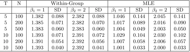
Table 1: Estimated coefficients for the non-dynamic panel
T N Within-Group MLE
β1= 1 SD β2= 2 SD β1= 1 SD β2= 2 SD
5 100 1.382 0.088 2.382 0.088 1.046 0.144 2.045 0.141 5 200 1.385 0.071 2.382 0.070 1.017 0.089 2.016 0.090 5 500 1.383 0.060 2.383 0.060 1.004 0.049 2.003 0.050 10 100 1.393 0.071 2.391 0.072 1.029 0.104 2.030 0.102 10 200 1.391 0.054 2.392 0.056 1.007 0.058 2.006 0.057 10 500 1.393 0.040 2.392 0.041 1.001 0.033 2.000 0.033
6 Simulation results
Non-dynamic panel. Data are generated according to (r = 2):
yit=δt+β1xit,1+β2xit,2+λ′ift+εit
xit,k =ι′λi+ι′ft+λ′ift+ξit,k, k= 1,2
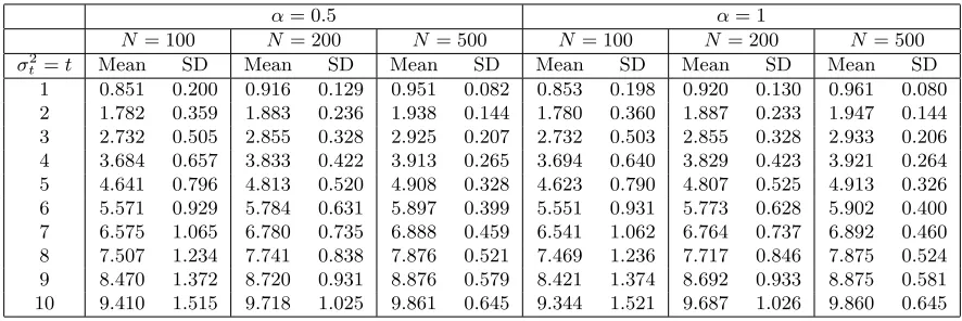
where εit ∼N(0, σt2) with σ2t =t, independent overt and i;ξit,k and the components ofλi and ft
are all iid N(0,1); ι′ = (1,1);β
1= 1, β2 = 2. So the regressors are correlated with the loadings, the
factors, and the their product. We consider heavy heteroskedasticity such that
D= diag(1,2, ..., T)
We set δt to zero, but time effects are allowed in the estimation.
While the usual within-group estimator is consistent under additive effects for non-dynamic models, it is inconsistent under interactive effects. To see the extent of bias, we also report the within-group estimator. The simulation results are reported in Table 1.
The columns are either the sample means (under the β coefficients) or the standard deviations (under SD) from 5000 repetitions. The within-group estimator is inconsistent since it cannot remove the correlation between the factor errors and the regressors. The MLE is consistent and becomes more precise as either N or T increases. The data generating process forxit (also admits a factor
structure) requires the projection of λi onto the entire path of xi. The usual Mundlak projection
on ¯xi is inconsistent. Not reported is the widely used Pesaran’s estimator, which does not perform
well. This corroborates the theory in Westerlund and Urbain (2013), who show that Pesaran’s estimator becomes inconsistent when the factor loadings in they equation are correlated with the factor loadings in the x equation. Our data generating process allows this correlation.
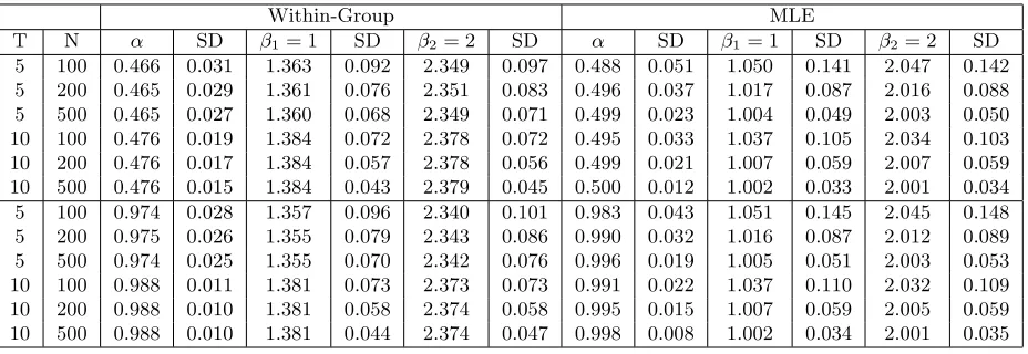
Dynamic panel. The y process is generated as (r= 2)
yit=δt+α yit−1+β1xit,1+β2xit,2+λ′ift+εit
all other variables are generated the same way as in the non-dynamic case. We again set δtto zero