Detecting Syntactic Change Using a Neural Part of Speech Tagger

Proceedings of the 1st International Workshop on Computational Approaches to Historical Language Change, pages 167–174 167

Detecting Syntactic Change Using a Neural Part-of-Speech Tagger

William Merrill,∗ †‡Gigi Felice Stark,∗ ‡ and Robert Frank‡

‡_{Department of Linguistics, Yale University, New Haven, CT, USA} †_{Allen Institute for Artificial Intelligence, Seattle, WA, USA}

[email protected]

Abstract

We train a diachronic long short-term memory (LSTM) part-of-speech tagger on a large cor-pus of American English from the 19th, 20th, and 21st centuries. We analyze the tagger’s ability to implicitly learn temporal structure between years, and the extent to which this knowledge can be transferred to date new sen-tences. The learned year embeddings show a strong linear correlation between their first principal component and time. We show that temporal information encoded in the model can be used to predict novel sentences’ years of composition relatively well. Comparisons to a feedforward baseline suggest that the tem-poral change learned by the LSTM is syntactic rather than purely lexical. Thus, our results suggest that our tagger is implicitly learning to model syntactic change in American English over the course of the 19th, 20th, and early 21st centuries.

1 Introduction

We define a diachronic language task as a stan-dard computational linguistic task where the in-put includes not just text, but also information about when the text was written. In particular, di-achronic part-of-speech (POS) tagging is the task of assigning POS tags to a sequence of words dated to a specific year. Our goal is to determine the extent to which such a tagger learns a repre-sentation of syntactic change in modern American English.

Our method approaches this problem using neu-ral networks, which have seen considerable suc-cess in a diverse array of natural language prosuc-cess- process-ing tasks over the last few years. Prior work usprocess-ing deep learning methods to analyze language change

∗

Authors (listed in alphabetical order) contributed equally.

†

Work completed while the author was at Yale Univer-sity.

has focused more on lexical, rather than syntactic, change (Hamilton et al.,2016;Dubossarsky et al.,

2017;Jo et al.,2017). One of these works,Jo et al.

(2017), measured linguistic change by evaluating a language model’s perplexity on novel documents from different years.

Previous work focusing on syntactic change uti-lized mathematical simulations rather than empir-ically trained models. Niyogi and Berwick(1995) attempted to build a mathematical model of syn-tactic change motivated by theories of language contact and acquisition. They found that their model predicted both gradual and sudden changes in a parameterized grammar depending on the properties of the languages in contact. In partic-ular, they used their simulation to study how verb-second (V2) order was gained and lost throughout the history of the French language. For several toy languages, their model found that contact be-tween languages with and without V2 would lead to gradual adoption of V2 syntax by the entire pop-ulation.

We use the Corpus of Historical American En-glish (COHA) (Davies, 2010-), an LSTM POS tagger, and dimensionality reduction techniques to investigate syntactic change in American En-glish during the 19th through 21st centuries. Our project takes the POS tagging task as a proxy for diachronic syntax modeling and has three main goals:

1. Assess whether a temporal progression is en-coded in the network’s learned year embed-dings.

2. Verify that the represented temporal change reflects syntax rather than simply word fre-quency.

2 Materials and Methods

2.1 Data

2.1.1 Corpus of Historical American English

The COHA corpus is composed of documents dat-ing from 1810 to 2009 and contains over 400 mil-lion words. The genre mix of the texts is bal-anced in each decade, and includes fiction works, academic papers, newspapers, and popular maga-zines. Because of computational constraints, we randomly selected 50,000 sentences from each decade for a total of 1,000,000 sentences. We se-lected an equal number of sentences from each decade to ensure a temporally balanced corpus. We put 90% of these into a training set and 10% into a test set. We also cut off all sentences at a maximum length of 50 words. We chose 50 words as our limit to avoid unnecessarily padding a large percentage of sentences. Only 6.95% of sentences in the full COHA corpus exceeded 50 words.

Texts in COHA are annotated with word, lemma, and POS information. The POS labels come in three levels of specificity, with the most specific level containing several thousand POS tags. We used the least specific label for our model, which still had 423 unique POS tags.

2.1.2 Word Embeddings

Our model utilized pre-trained 300-dimensional Google News (Mikolov et al.,2013) word embed-dings that were learned using a standard word2vec architecture. When there was no embedding avail-able for a word in the corpus, we assigned the word an embedding vector drawn from a nor-mal distribution, so that different unknown words would have different embeddings. Due to compu-tational constraints, we only included embeddings for the 600,000 most common words in the vo-cabulary. Other words were replaced by a special symbolUNK.

2.2 Methods

2.2.1 Network Architecture

We used a single-layer LSTM model.1 For a given sentence from a document composed in the year with embedding t, the model’s input for the ith

word in the sentence is the concatenation of the word’s embeddingxiandt. For example, consider

a sentencehello world!written in 2000. The input

1_{https://github.com/viking-sudo-rm/}

DiachronicPOSTagger

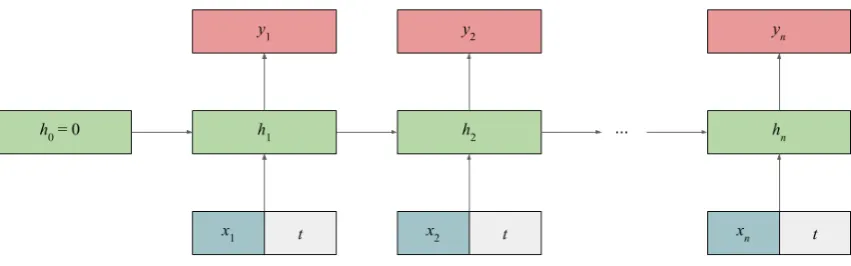
corresponding tohellowould be the concatenation of the embedding forhelloand the embedding of the year 2000. A diagram of this architecture can be seen inFigure 1.

An interesting feature of our approach is that a single model can learn information about differ-ent time frames. Thus, in principle, learning from sentences in any year can inform predictions about sentences in neighboring years.

The word embeddings were loaded statically. In contrast, year embeddings were Xavier-initialized and learned dynamically by our network. Thus, we did not explicitly enforce that the year embed-dings should encode any temporal progression.

We gave both the word embeddings and year embeddings a dimensionality of 300. We picked the size of our LSTM layer to be 512. Due to the size of our training set and our limited com-putational resources, we ran our network for just one training epoch. Manual tweaking of the learn-ing rate and batch size revealed that the network’s performance was not particularly sensitive to their values. Ultimately, we set the learning rate to 0.001 and the batch size to 100. We did not in-corporate dropout or regularization into our model since we did not expect overfitting, as we only trained for a single epoch.

In order to calibrate the performance of our LSTM, we trained the following ablation models:

• An LSTM tagger without year input

• A feedforward tagger with year input

• A feedforward tagger without year input

All taggers were trained with identical hyper-parameters to the original LSTM. For the feedfor-ward models, the LSTM layer was replaced by a feedforward layer of size 512. The lack of recur-rent connections in the feedforward models makes it impossible for these models to consider inter-actions between words. Thus, these models serve as a baseline that only considers relationships be-tween single words and their POS tags–not syntax.

2.2.2 Analyzing Year Embeddings

Figure 1: LSTM architecture. The input to the LSTM at each step is the concatenation of the current word’s embedding and the corresponding document’s year embedding. Each output is the predicted POS tag for the current word.

that requires no hyperparameter tuning. We cal-culated the correlation between the first principal component of the embeddings and time.

Both the LSTM and feedforward models cap-ture lexical information. However, due to its re-current connections, the LSTM model is also in-formed by syntax. To evaluate whether the rela-tionship between years and learned embeddings was due to syntax or simply word choice, we com-puted the correlation between the first principal component of the embeddings and time for both the LSTM and feedforward models. The differ-ence between the LSTM and feedforwardR2

val-ues reflects the degree to which the LSTM’s repre-sentation of time is informed by syntactic change.

2.2.3 Temporal Prediction

We evaluated the ability of our model to predict the years of composition of new sentences. Be-cause this task is difficult for a single sentence, we evaluated model performance at the aggregate level, bucketing test sentences by either year or decade. As the year grouping is much more nar-row, model performance when these buckets are used should be worse. We report both year and decade metrics to evaluate the extent to which our model is effective at different levels of specificity. We used our model to compute the perplexity of each sentence in a given bucket at every possible

year (1810-2009). We then fit a curve to perplex-ity as a function of year using locally weighted scatterplot smoothing (LOWESS). These curves provide clear interpretable visualizations that dis-count extraneous noise. We took the year cor-responding to the LOWESS curve’s global mini-mum as the predicted year of composition for the sentences in the bucket.

We compared the effectiveness of the LSTM and the feedforward taggers for temporal tion. For decade buckets, we quantified the predic-tive power of each model by calculating the aver-age distance across decades between each decade bucket’s middle year and predicted year of com-position. Similarly, for year buckets, we measured the average distance between the predicted and ac-tual years of composition. For both metrics, the naive baseline model assigns each bucket a pre-dicted year of 1910 (the middle year in the data set), which results in a metric value of 50.0 for both decade and year buckets.

3 Results

3.1 Tagger Performance

Feedforward LSTM

Year 82.6 95.5

No Year 77.8 95.3

Table 1: Test accuracies for all architectural variants. The networks differed in whether year information was included as input and whether the hidden layer had LSTM or feedforward connections.

Feedforward LSTM

Year 82.6 95.6

No Year 77.7 95.4

Table 2: Training accuracies for all architectural vari-ants.

relatively high test accuracy suggests that the tag-ger is legitimate. The LSTM without year input performed marginally worse with a 95.3% test ac-curacy (see Table 1). These results suggest that temporal information slightly aids tagging.

The feedforward taggers with and without year input had test accuracies of 82.6% and 77.8%, re-spectively (again, see Table 1). As feedforward networks, unlike LSTMs, do not take into account relations between words, it makes sense that their POS tagging performance is much lower. Addi-tionally, these results bolster the idea that year in-put improves tagging performance.

To justify not implementing dropout, regular-ization, or other techniques to combat overfitting, we calculated the training set accuracies of each model. For each type of the model, the training set accuracy was comparable to the test set accuracy (seeTable 2). Thus, our models did not overfit.

3.2 Analyzing Year Embeddings

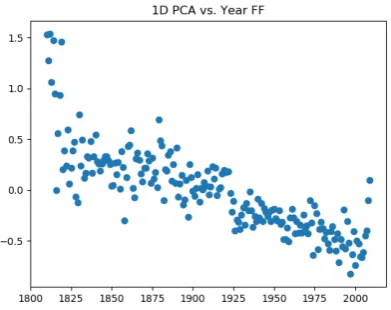
When we plotted the LSTM-learned year embed-dings using one-dimensional PCA, a clear linear relationship (R2 = 0.89) between the years and the first principal component emerged (see Fig-ure 2). These results suggest that the most signif-icant information in the year embeddings encodes the relative position of each year within a chrono-logical sequence. As the first principal compo-nent seems to encode temporal information well, we did not see a need to investigate additional principal components. This strong linear correla-tion suggests that, at the aggregate level, change is monotonic and gradual over time. Even if specific changes do not occur monotonically, the aggrega-tion of these changes allows the network to learn a

Figure 2: The first principal component of the LSTM year embeddings correlate strongly with time (R2 ₌

0.89).

Baseline Feedforward LSTM

Decade 50.0 26.6 12.5

Year 50.0 37.5 21.9

Table 3: Average distance between each time period’s center and the year that minimizes the perplexity value of the corresponding LOWESS curve. For the decade-level metric, the “center” is the middle year of the decade (1815 for 1810s). For the year-level metric, the “center” is the year itself (1803 for 1803).

Figure 4: The 1840s LOWESS curve for the LSTM. The year 1848 corresponds to the minimum perplexity.

monotonic representation of change.

The feedforward network’s temporal correla-tion was weaker (R2 = 0.68) (seeFigure 3). The discrepancy between the LSTM and feedforward

R2 values indicates that the LSTM does not only identify effects of lexical change, but also syntac-tic change.

3.3 Temporal Prediction

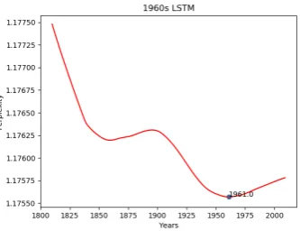
For both year and decade buckets, the LSTM pre-dicted the years of composition of new sentences much better than the feedforward neural network or the baseline (seeTable 3). We also confirmed our hypothesis that for both types of models the prediction error for decade buckets would be lower than for year buckets. Examples of some of the LSTM perplexity curves can be seen in Figures

4, 5, 6, 7, and8. Examples of some of the feed-forward curves can be seen in Figures 9 and10. For all decades, the feedforward year of composi-tion prediccomposi-tions tended to be skewed towards the middle years of the data set (late 1800s and early 1900s). These findings suggest that the represen-tation of syntactic change learned by the LSTM can be leveraged to date new text.

We examined sample sentences whose years of composition were predicted well. We

sam-Figure 5: The 1880s LOWESS curve for the LSTM. The LSTM’s prediction for this decade is weaker than for the other selected decades. The year corresponding to the minimum perplexity is 1859.

Figure 6: The 1920s LOWESS curve for the LSTM. The year 1929 corresponds to the minimum perplexity.

Figure 8: The 2000s LOWESS curve for the LSTM. The year 2009 corresponds to the minimum perplexity.

Figure 9: The 1820s LOWESS curve for the feedfor-ward tagger. For this decade, the feedforward net-work is somewhat off as the year 1883 corresponds to the minimum perplexity. For the feedforward network, there is an evident bias across decades towards the late 1800s and early 1900s, which are the middle years of the data set.

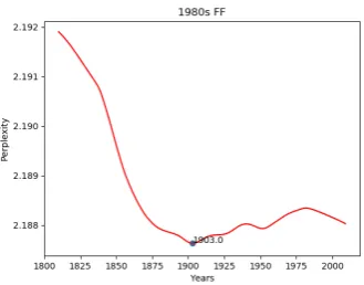
Figure 10: The 1980s LOWESS curve for the feedfor-ward tagger. The feedforfeedfor-ward network does not per-form well for this decade. The year corresponding to the minimum perplexity, 1903, is somewhat far from the 1980s. Again there is an evident bias in prediction towards the middle years of the data set.

pled 1,000 test data set sentences. Of sentences longer than five words, we examined the ten sen-tences with the smallest errors (distance between the LSTM-predicted year of composition and the actual year of composition). For each of these sen-tences, we also calculated the error assigned to the sentence by the feedforward model in order to de-termine the extent to which syntax aided these pre-dictions. These ten sentences are detailed in Ta-ble 4. Generally for these sentences, the feedfor-ward error was comparable to or larger than the LSTM error, which suggests that syntactic infor-mation improved prediction for these sentences.

Sentence 1 (again, see Table 4) was one of seven sentences whose year of composition was predicted perfectly. This sentence’s predicted year of composition was the same as its actual year of composition (1817). It makes sense that this sen-tence was predicted well since its syntax is qualita-tively archaic. For example, it uses the uninflected subjunctive formshinewhereas modern American English would prefershines.

4 Conclusion

Through our PCA analysis of the year embed-dings, we found that the LSTM learned to rep-resent years in a chronological sequence without any biases imposed by initialization or architec-ture. The LSTM also effectively predicted the year of composition of novel sentences. Relative per-formance on these tasks indicates that the LSTM learns a stronger representation of time than the feedforward baseline. Therefore, the diachronic knowledge learned by the LSTM must encompass syntactic–not just lexical–change.

Year Error

Sentence Pred True FF LSTM

1. it is of great consequence, that we adorn the religion we profess, and that our light shine more and more that we grow in grace as we advance in years, and that we do not resemble the changing wind or the inconstant wave.

1817 1817 86 0

2. what extenuations or omissions had vitiated his former or recent narrative; how far his actual performances were congenial with the

deed which was now to be perpetrated, i knew not. 1827 1827 0 0

3. that an unlimited power of making gifts could be narrowed down, by any process of reasoning, to the idea of a grant to an indian, a

reward loan informer, and much less to a mere sale for money. 1833 1833 16 0

4. “amiable, generous, kindhearted woman! thou wert anxious to procure for thy poor, afflicted, aged mother, all the repose which her advanced life seemed to require, to wipe away the tear from her dimmed eye and farrowed cheek, and as far as

1817 1817 10 0

5. count when shall we meet again? ther. _{1821 1821 11 0}

6. in some instances, upon killing them after a full year’s depriva-tion of all nourishment, as much as three gallons of perfectly sweet

and fresh water have been found in their bags. 1838 1838 21 0

7. that’s a good way to think about me.

1996 1996 12 0 8. the contention between the wife of abraham and her egyptian

handmaid, has already been the subject of animadversion; but although their histories are considerably blended, some features in the character of the latter, and some affecting circumstances of her life, have been hitherto omitted,

1816 1817 0 1

9. but what happens when your erotic adventure is stifled by an unwelcome companion, such as a roommate? masturbating in a UNK situation does pose some problems, but where there is a will, there is a way.

2003 2002 22 1

10. it is UNK in truth we are an united people it is true but we are, family united only for external objects; for our common defence, and for the purpose of a common commerce; sharing, in com mop, the UNK and privations of war

1826 1827 3 1

References

Enoch Olad Aboh. 2015. The Emergence of Hybrid

Grammars: Language Contact and Change.

Cam-bridge Approaches to Language Contact. CamCam-bridge University Press.

Mark Davies. 2010-. The corpus of historical Ameri-can English: 400 million words, 1810-2009.

Haim Dubossarsky, Daphna Weinshall, and Eitan Grossman. 2017. Outta control: Laws of semantic change and inherent biases in word representation

models. InProceedings of the 2017 Conference on

Empirical Methods in Natural Language Process-ing, pages 1136–1145, Copenhagen, Denmark. As-sociation for Computational Linguistics.

William L. Hamilton, Jure Leskovec, and Dan Jurafsky. 2016. Diachronic word embeddings reveal statisti-cal laws of semantic change. InProceedings of the 54th Annual Meeting of the Association for Compu-tational Linguistics (Volume 1: Long Papers), pages 1489–1501, Berlin, Germany. Association for Com-putational Linguistics.

Eun Seo Jo, Dai Shen, and Michael Xing. 2017. Back-prop to the future: A neural network approach to

linguistic change over time. Manuscript, Stanford

University.

Tomas Mikolov, Kai Chen, Greg Corrado, and Jeffrey Dean. 2013. Efficient estimation of word represen-tations in vector space.CoRR, abs/1301.3781.