Estimation for Nonnegative First-Order Autoregressive
Processes with an Unknown Location Parameter
Andrew Bartlett, William McCormick University of Georgia, Athens, USA
Email: [email protected]
Received September 10, 2012; revised October 10, 2012; accepted October 17, 2012
ABSTRACT
Consider a first-order autoregressive processes XtXt1Zt, where the innovations are nonnegative random vari-ables with regular variation at both the right endpoint infinity and the unknown left endpoint θ. We propose estimates for the autocorrelation parameter and the unknown location parameter θby taking the ratio of two sample values cho-sen with respect to an extreme value criteria for and by taking the minimum of XtˆnXt1 over the observed series, where ˆn represents our estimate for . The joint limit distribution of the proposed estimators is derived using point
process techniques. A simulation study is provided to examine the small sample size behavior of these estimates.
Keywords: Nonnegative Time Series; Autoregressive Processes; Extreme Value Estimator; Regular Variation; Point
Processes
1. Introduction
In many applications, the desire to model the phenomena under study by non-negative dependent processes has increased. An excellent presentation of the classical the- ory concerning these models can be found, for example, in Brockwell and Davis [1]. Recently, advancements in such models have shifted focus to some specialized fea- tures of the model, e.g. heavy tail innovations or non- negativity of the model. In this paper we examine the behavior of traditional estimates under conditions leading to non-Gaussian limits. For example, the standard ap- proach to parameter estimation within the AR(1) process is through the Yule-Walker estimator;
1
1 1
2 1 1
1
ˆ ,
1
where .
n
t t
t
LS n
t t
n t t
X X X X
X X
X X
n
(1.1)
A slightly different approach presented in Mathew and McCormick [2] used linear programming to obtain esti- mates for and under certain optimization con- straints. While there are many established methods to estimate the autocorrelation coefficient in an AR(1) mo- del, there are just a few approaches on estimating the unknown location parameter in an AR(1) model. One,
was mentioned in McCormick and Mathew [2] where they considered
1
range range 1 range
1
ˆ ˆ , where ˆ t j ,
j j
t j
X X
X X
X X
t and j provides the index of the maximal and minimal Xi respectively for 1 i n.
In this paper we examine estimation questions and asymptotic properties of alternative estimates for and respectively, relating to the model
1 , 1,
t t t
X X Z t
where 0 1, 0 and
Zt is an i.i.d. sequenceof nonnegative random variables whose innovation dis- tribution F is assumed to be regularly varying at infinity with index and regularly varying at with index , where , denotes the unknown but positive left endpoint. As a result of not restricting the innovations
Zt to be bounded on a finite range, we can firstestimate the autoregressive parameter through re- gular variation at infinity and then estimate the positive but unknown location parameter through regular vari- ation at , the left endpoint.
dure had a major contribution on the estimation of posi- tive heavy tailed time series. With these considerations in mind, Raftery [3] determined the limiting distribution of the maximum likelihood estimate for the autocorrelation coefficient . As a result, the estimator
1 1
ˆ n t ,
n t
t
X X
∧
(1.2)was considered. The realization of this estimator was the stepping stone for the work done in this paper along with Davis and McCormick [4] which first considered this alternative estimator and used a point process approach to obtain the asymptotic distribution of the natural esti- mator ˆn. This was done in the context that the in-
novations distribution F varies regularly at 0, the left endpoint, and satisfy some moment condition.
The work presented in this paper is an extension of the work done in Davis and McCormick [4] including the following contributions to dependent time series with heavy-tail innovations. The first contribution involves the development of estimates for the autocorrelation coeffi- cient and unknown location parameter under regular vari- ation at both endpoints, with a rate of convergence
1n n , where is slowly varying function. The second contribution involves using an extreme value method, e.g. point processes to establish the asymptotic distribution of the proposed estimators and weak con- vergence for the asymptotically independent joint dis- tribution. An initial observation is that our estimation procedure is especially easy to implement for both and . That is, the autoregressive coefficient in the causal AR(1) process is estimated by taking the mini- mum of the ratio of two sample values while estimation for the unknown location parameter was achieved through minimizing Xt ˆnXt1 over the observed series.
This naturally motivates a comparison between the estimation procedure presented in this paper and the standard linear programming estimates mentioned above, since within a nonnegative AR(1) model the linear programming estimate reduces to the estimate proposed, namely, min1 t n
X Xt t1
, where
Xt denotes theAR(1) process. This comparison along with the com- parison between Mathew and McCormick’s [2] opti- mization method and Bartlett and McCormick [5] extreme value method was performed through simulation and is presented in Section 3. The results found appear to demonstrate a favorable performance for our extreme value method over the 3 alternative estimators.
The main proofs in this paper rely heavily on point process methods from extreme value theory. The essen- tial idea is to first establish the convergence of a se- quence of point processes based on simple quantities and then apply the continuous mapping theorem to obtain
convergence of the desired statistics. More background information on point processes, regular variation, and weak convergence can be found in Resnick [6]. Also, a nice survey on linear programming estimation proce- dures and nonnegative time series can be found in Anděl [7], Anděl [8], and Datta and McCormick [9], whereas more applications on modeling the phenomena with heavy tailed distributions and ensuing estimation issues can be found in Resnick [10].
The rest of the paper is organized as follows: asympto- tic limit results for the autocorrelation parameter , unknown location parameter , and joint distribution of
, are presented in Section 2, while Section 3 is concerned with the small sample size behavior of these estimates through simulation.2. Asymptotics
The following point process limit result is fundamental. Since the result makes no use of an ARMA structure, we present it for more general linear models subject to usual summability conditions on the coefficients. In that regard
for this result, we assume that is the sta-
tionary linear process given by
, 0
n X n
j
0
n j n
j
X c Z
with
0 j
j
c
for some 0 , 1. Further-more for this result we may relax our assumptions on the innovation distribution and we require that Z1 has a regularly varying tail distribution, i.e.,
1
,P Z x x x x0 for a slowly varying fun-
ction and the innovation distribution is tail balanced
11
11
and as .
P Z x P Z x
p q
P Z x P Z x
x
Define point processes
1
1,
1
, 1
n k k n
n b X Z
k
n
and let 1 jk
k
denote PRM
on 0
0 where has Radon-Nikodym derivative with respect to Lebes- gue measure
1 0,
1 ,0
d
1 1
d x p x x q x x .
Let
Zi k, ,i0,k1
be an iid array with , 1d i k
Z Z
and independent of 1 jk
k
. Define , ,
1 0 c j Zi k i k
k i
Our basic result is to show that Mp
0 with the topology of vague convergence
equipped
in d n
which is close in statement and spirit to Theorem 2.4 in Davis and Resnick [11]. In view of the commonality of the two results, we present only the needed changes to the Davis and Resnick proof to accommodate the current setting. Aside from keeping track of the time when points occur, i.e. large jumps, the difference in the point pro- cesses considered here with those in Davis and Resnick [11] is the inclusion of marks, i.e. the second component
of the point
1 . This complication induces an1,
n k k
b X Z
.
additional weak dependence in the points which is addressed in Lemma 2.2 through a straight forward blocking argument. First, we establish weak convergence of marked point processes of a normalized vector of in- novations. For a positive integer m define
1 1
, , ,
m
k Z Zk k Zk m
Z
and point process
1 1 , 1 , 1 m n k k
n m
n b Z
k n
Z Let denote the standard
basis vectors for . Define an associated marked point process with the first component placed on an axis by
0, ,1, , 0 ,1
i i m
e
m
1 ,
1 1 n k i k i n m
m
n b Z e Z
k i
In the following Lemma, we show that and
are asymptotically indistinguishable in the following sense. Let
m n
n m
0 0
m m
and . Consider
the class of rectangles 0
Em
1 , : , , and , i i m iR x R c d
x R x
E Lemma 2.1. As n tends to infinity
m
m
p 0 for alln B n B B
.
Proof. Following the proof presented in Proposition 2.1 of Davis and Resnick [11], suppose that B
i
is
such that for some 1 , i As
noted in Davis and Resnick [11] for all , one has . Observe that
i m B e
i .
i
d
0 i
c
1
1 , 2
, ,
, ,
n k i k i
m m
n n i i
n i
i i
b Z Z
k i
B c d
c d x
e x (2.1)Similarly let and .
Then
0 i i i
c c d i idi0
, , , , , , m n mn i i
m
n i i
m
n i
i i
B
c d c d c d x
c d x
E x
, (2.2)where y
y1, , ym
Ei according to yi
c d,and yi
c di, i
. Note that
1 1
,
1 , 1
1 . m
n i
i i
n n
E E x
nP Z c d Z c d
b b o (2.3)
Thus from (2.1)-(2.3) we obtain
1
1
2 1 1 1
as .
m m
n n
i i
n
E B B
i P Z c d o o
b n (2.4)
Then the result follows as in Davis and Resnick [11], Proposition 2.1, completing the proof. □
Lemma 2.2. Let and be the point pro-
cesses on the space defined by
m n
E
m
m 0
1 , ,
1 1
and
m m
n k k m k k
n
m m
n b Z Z j Y
k k
where
Yk m,k1
is an iid sequence with
1 1, ,
d m
m
Z Z
Y and is independent of
1 jk
k
. Thenin Mp
E , m d m.
n
Proof. We employ a blocking argument to establish this result. Let be a sequence of integers such that rn
n
r r as n and r o n
. Let h n r and l m . Define blocks
, , , 11 1, , ,
1, ,
for 1 and 1, , .
n s
n s
n h
I r s rs l
J rs l rs
s h J rh n
Then it is clear that for s t
, , , ,0 , ,0k i n s
k i n t
Z k I i m
.
Z k I i m
Write 1 1 , , , ,
, m and , m
n k k m n k k m
n s n s
m m
n s n t
b Z b Z
k I k J
Then
1
,
1 1
.
h h
m m
n n s
s t
n t,m
B
(2.5)
Let BE be a disjoint union of rectangles
1
j i i
B
(2.6) where Bi
c di, i
Ri with 1
,
m
i l il il
R
x y . LetF F
denote the mean measure ofwhich is PRM
m
on . To complete the proof we
first show that for all sets of the form given in (2.6) that
E B
lim m 0 exp .
n
nP B B
(2.7)
The above limit result follows from the easily veri- fiable relations:
,1 , ,1 0 0 ; m mn n h
m h
n
P B B
P B
(2.8)
2, , 1 2
for 1 ;
m m
n s k n s l
r
P B B O
n
k l j
(2.9)
, 1 2 , 2 1 1 1 ; j mn s i
i
j m n s i i
P B
r
P B O
n
(2.10)
,1 1
1
m
n i i
r
P B B o
n
1 ; (2.11)
and
1 , 1
0 as .
h m p n t t B n
B (2.12)Indeed, in view of (2.5) and (2.12), (2.7) is equivalent to showing
, 1
lim h m 0 exp
n s
nP s B
(2.13)and the above relation holds by (2.8), (2.10), and (2.11), viz.
, ,1 1 1 10 1 1
1
exp .
h h
m m
n s n
s h j i i j i i
P B P B
r B o r n
n B
It is immediate that for a rectangle
, 1
,
m
i i i
B c d
x y E we have m
lim n .
nE B B (2.14) Therefore the result is seen to hold by (2.7) and (2.14) by application of Theorem 4.7 in Kallenberg [12]. □
Lemma 2.3. Let n m and be point processes
m
m
on the space E0
1 , 1 , , 1 1
, 1 and
m i i k
n k k
n m
m m
n b Z j e Zk
k k n
Z 1 i
Then in Mp
E , m d m.
n
Proof. We begin by applying the argument used in Theorem 2.2 of Davis and Resnick [11] with the modi- fication that the relevant composition of maps of point processes is given by
1 1 1 1 , , , , ,
1 1 1
, , 1 1 , . 1 1 , , , , k mk k k mk k k
k k k m mk
k i ik
u v v u v u v
k k k
u e v u e v
k k
m
u e v k i
Each map being continuous, the composition is a con- tinuous map from Mp
0m
to
0
m p
M
with each space being equipped with the topology of vague convergence. Therefore by the continuous mapp- ing theorem and Lemma 2.2 we obtain
1 , , ,
1 1 1 1
.
k i i k n k i k i
m m
m d
n b Z e Z j Z
k i k i
m
e
(2.15)
Finally we complete the proof by Lemma 2.1 and (2.15) arguing as in Davis and Resnick [11].
We are now ready to present our fundamental result.
Theorem 2.1. Let n and be the point processes
on the space E0 defined by
1
,
1, ,
1 1
, 1 and
i k i k n k k
n
n b X Z c j Z
k k n
0 i
where 1 jkk
is PRM
and
isan iid array with
, , 0, 1
i k
Z i k
, 1
d i k
Z Z and independent of
1 jk
k
. Then in Mp ,
E. d n
Remark. Apart from considering a time coordinate
Cormick [2] consider essentially the same point process limit result. However, their result gave a wrong limit point process. This error is corrected in the current paper.
Proof. Observe that the map
1 1
10
, , , m
k k k m i k i
i
z z z c z
0
m
induces a continuous map on point processes given by
1 1 1 1 1 0
, , , ,
,
1 1
. m
k k k m k
j k j k j
z z z z
c z z
k k
Thus we obtain from Lemma 2.3 that
1
1 ,
1 0
1 , . ,
1 1
.
m
i k i k n i k i k
i
n
d
c j Z
b c Z Z
k k i
(2.16)The result now follows from (2.16) by the same argu- ment in Davis and Resnick [11] to finish their Theorem 2.4.
Returning to the AR(1) model under discussion in this paper and the estimate ˆn given in (1.2), we obtain the following asymptotic limit result.
Theorem 2.2. Let be the stationary solu-
tion to the AR(1) recursion
, 0
t
X t
t
1
t t
X X Z and
1
1
ˆ t
n
t
n t
X X
∧
. Under the assumptions that 0 1 and the innovation distribution F has regularly varying right tail with index and finite positive left endpoint,
ˆ
lim e x EW for all 0,
n n
n P b x x
where i 0 ii
Z W
∧
and bn F
1 1n
.
Proof. For x0 define a subset
21 2 1 2
1
, : , 0,
x
x
Q x x x x x
x .
Then note that for the point processes
1 1,1 n k k
n
n b X Z
k
, we have
1 1
1
ˆ
0 .
n k
n x k n n
n k
Z
Q x b
b X
∧
xApplying Theorem 2.1 in the case of an AR(1) process
so that i, 0, we have
i
c i
, ,
1 0
. k i k
d
n i j Z
k i
Note that as a subset of E
0,
,
, the set xQ is a bounded continuity set with respect to the limit point process so that
,
1 0 1
ˆ
lim n n x 0
n
i k k
i
k i k
k k
P b x P Q
Z W
P x P
j j
x
∧∧
∧
where
0 i , , 1
k i i k
W Z k
∧
is an i.i.d. sequence in-dependent of
j kk, 1
. Let ,
1 . k k
j W k
(2.17)
Then by Proposition 5.6 in Resnick [10], we have that if G denotes the distribution of W1, then is a
Poisson random measure on E with mean measure
G
, where
d 11
0, d
x x x x
. Using
(2.17) we can write
1 0 exp
k
x x
k k W
P x P Q Q
j
∧
.Since
Qx x EW , the result follows.Corollary 2.1. Under conditions given in Theorem 2.2,
.
ˆ a s .
n
Proof. Since bn F
1 1 n
we have
ˆ p
n
. But this implies ˆ a s. .
n
since ˆn and is non-increasing.
Let us now define our estimate of :
1
ˆ ˆ ,
n
n t I Xt nXt
∧
where we define the index set
:1 and 1
n t
I t t n X a bn n
where 0 1
is a fixed value.
Lemma 2.4. Under the assumptions that F is regularly
varying with index at its positive left endpoint and F is regularly varying with index at infinity,
its right endpoint, and , then
1 ˆ 0, as ,
n
p
n n t
t I
a Z n
∧
where anF
1n . Furthermore, for any y0
1
1 1 ˆ lim
lim e .
n n
n
n
y
n t
n t
P a y
P a Z y
∧
Proof. Since , we have limna bn n . Therefore since
bn
ˆn
,n1
is a tight sequenceby Theorem 2.2 and since maxt InXt 1
a bn n
1
with
1 1 ˆ 0. n pn n t I t
a X
∨
The first statement now follows since
1 1
1
ˆ ˆ .
n n
n n t I t n n t I t
a Z a
∧
∨
X
0
For the second statement observe
1 1 1 1 1 1 1 1 1 0 1 0 and 1 . n n nn t I t n t t
n
n t t n t I t
t n n n t
t n
n n n
P a Z y P a Z y
P a Z y a Z
P X a b a Z y
nP X a b P Z a y o
∧
∧
∧
∧
(2.18) The result for the second statement now follows from (2.18) and the first part of the lemma. Finally, the iden- tification of the limit distribution is well known. □A useful observation follows from this lemma which we state as a corollary.
Corollary 2.2. Under the assumptions of Lemma 2.4
for any x y, 0
1 1 1 ˆ ˆ lim , ˆ ,n n n n
n
n
n n n t t
Pb x a y
P b x a Z y
∧
Proof. By Lemma 2.4 we have
1 1 ˆ ˆ lim , ˆ , nn n n n
n
n n n t I t
P b x a y
P b x a Z y
∧
0The result then follows from
1 1 1 1 1 1 ˆ 0 1 1 1 . n n n n nn t I t n t t
n
n t I t n t t
E b x
a Z y a Z y
P a Z y P a Z y
∧
∧
∧
∧
□Corollary 2.2 allows a simplification in determining the joint asymptotic behavior of
ˆ ˆn, n by allowing us to replace ˆn with min1 t nZt. The next lemma will provide another useful simplification—this time on ˆn.For a positive integer m define
1
0 . m m i t t i i
X Z
Lemma 2.5. Let Un m and Un be defined as
1
1 1 1 1 1 and . n n
m t t
n t m n t
n t n t
Z Z
U U
b X
b X
∧
∧
Then for any 0
lim lim nm n 0.
m n P U U
Proof. We first note for any positive M that
2
1 1
1 1
.
m m
n n n n m
n n m n m n n
P U U P U U
U U
P M P U M
U U
In order to calculate 1 m 1 n n P U U
we partition
t
X . That is, we write
m m
t t t
X X X
where m j
t t
j m j
X Z
, so that
1 1
1 1 1
0 .
m m
n n n
t t t
t t t
t t
X X X
Z Z Z
∨
∨
∨
1t
i m
Define point processes
1
,
1 , ,
1 1
and i
m
k i k n t t
n
m m
n j Z
b X Z
t k
where
j kk, 1
and
Zi k, ,k1,i0
ihave the dis- tributional properties given in Theorem 2.2. Applying Theorem 2.2 with ci for i and equal to 0
otherwise, we obtain
m
ci
m d m. n
Then letting for x0
, : 0, ,and , xu
u v u v x
v we have
1 1 1 limlim 0 0 .
n
m
n t t
n t
m m
n x x
n
P b X Z x
P P
∨
Setting , 1 , and m k k i m mk i m j V
we have
1 0 0 , mx k k k
m x
P P j V
P
∨
m x. where
, : 0, ,and
x u v u v uvx
Since m is Poisson random measure with mean
measure m Hm where and
1
m m
V H
1 ,
m m x x E V
we obtain
1 1 1 1lim exp .
n
m m
n t t
n P t b X Z x x E V
∨
Next since 1 1 11 1 n m ,
n t m t n t n b X U Z U
∨
we have for large n that
12 1 2
1 2 1 2 1 1 1
2 1 exp
2 . m n n t m t n t n m m b X
P M P
U Z
U
M E V
M E V
∨
MTherefore, since 1
m m
V ,
2
1 1
lim lim m 0.
m n n n P M U U
Next, note that from the limit law for the maximum obtained above, by replacing 1 with
m t
X 1
m t
X and by
taking reciprocals, we derive the limit law for minimum,
1 1 1 lim 1 exp n m tn t m
n
n t
m Z
P U x
b X x EW
∧
(2.19)where Wm has the distribution of
∧
mi01Zi k, i. Thus,for any integer m1,
lim m 1 exp .
n
n P U x x
Thus for any 0, we have for M large enough that
1 lim sup sup m
n
n m
P U M
completing the proof. □
With Lemma 2.5 in hand we can now focus our atten- tion to the limiting joint distribution of
, 1
.m n
n t t
U
∧
ZThis will be accomplished by a blocking argument. To that end for a fixed positive integer , let k rn n k
and define blocks for i1, , n rn by
1 1, ,
and 1, ,
i n n
i n n
,
J i r ir q
J ir q ir
where is a positive integer greater than . Further- more, let
q m
0 n n 1, , .
J r n r n
Now we define the events
1
1 1
: or
1, ,
l
i i m n l
n l
n
Z
l J x a Z y
b X i l , and
1
1 1
: or
0, ,
l
i i m n l
n l
n
Z
l J x a Z y
b X i l ,
where ln n rn. We begin by showing that the events
i
are negligible.
Lemma 2.6. For anyx y, 0
0
lim n 0.
l i n i P
Proof. Observe that
1 1 1 1 1 0 1 l m mn l n l
m i i Z
nP x nP x
b X b X
x x
(2.20)
and
1
.n l
nP a Z y y (2.21)
Thus for some constant and any c n1,
=0 n
l i i
P c
k nestablishing the lemma.
Define events Ai and Bi by
1 1 1 :and : .
l
i i m
n l
i i n l
Z
A l J x
b X
B l J a Z y
The following result provides the asymptotic behavior of the probability of these events.
Lemma 2.7. For any x0,y0, we have as k
1
lim i m andlim i .
n n
y
P A x EW P B
k k
Proof. Since the events Ai are independent, we have
1 1 1 1 1 1 , , . k l i m
i n l
k l
m
n l
Z
P x l
b X
Z
P x l J
b X
J
Using Lemma 2.6 we have that
1 1 1 1 1 1 1 1 1 1 , 1 , . n l m l n l k l i m
i n l
k l m n l Z P x b X Z
P x l J
n b X
Z
P x l J O
n b X
∧
O From (2.19) we showed that
1 1 1 lim1 exp .
n m t n m n t n t m Z
P U x
b X x EW
∧
Hence using this limit law on
1
1 1
m n
t Z b Xt n t
∧
, weobtain
1 1 1lim lim ,
exp . k l m k n n l m Z
P x l
b X
x EW J Thus,
lim i m ,as .
n
x
P A EW k
k
(2.22)
Similarly using the result of Lemma 2.4, we obtain
lim i ,as .
n
y
P B k
k
(2.23)
Hence the lemma holds. □
Lemma 2.8. For some constant c
i i
.
i iP AB cP A P B
Remark. Since the cardinality of Ji depends on
which depends on and the events n
r
k Ai and de-
pend on , and i
B
n P A
i
P B
i depend on k and n.The conclusion of this lemma provides that for all and , there is a constant dependent on no parameters for which the inequality stated there holds.
k n
Proof. To calculate the intersection we define the following sets
1 1,i 1, 2 : ,1 2 iand 2 1 1 ,1
K K l l l l J l l m l
and
2 2,i 1,2 : ,1 2 i and 2 1 1 ,1 .
K K l l l l J l l m l Now for l1 1 m l2 l1 1 and n sufficiently large,
2 1 1 1 1 2 2 1 1 1 1 1 1,0 1 1 . l n l m n l l il i n
i l l i m
l n
Z
x a Z y
b X
Z
Z b
x
Z a y
It then follows from (2.20), (2.21), and independence that
1 1 1 2 2 1 1,0 1 2 1 1 . l il i n
i l l i m
l n
Z
P Z b
x
Z a y
O n
If l1 l2 l, we have
1 1
1
1 1 2
1 d . n l n l m n l a y m l n Z
P x a Z
b X
z
P X F z O
b x n
yTherefore, for some constant c
12
1 2 2 1
1 1 , 1 . l n l m
l l K n l
Z
P x a Z
b X c nk
y
In order to handle set K1, observe from construction
of the blocks Ji and set K1 that if then
the events
1 2
1,
l l K
1 2 1 1 1 1 and l n l m n l Zx a Z y
b X
are independent. Thus, if we define
as anindependent copy of
, i
Z i
1 21 2 1 1
1
2
1 2 1 1
1 1 , 1 1 1 , 1 2 l n l m
l l K n l
l
n l
m
l l K n l
i i i i
Z
P x a Z
b X
Z
P x a Z
b X
P A B P A P B c k
y y ywhere and where we
used Lemma 2.7 in the last step. Thus, we have that for some constant
: 1
i i n l
B l J a Z
c
21 2 1 1
2
1 2 2 1
1 1 1 , 1 1 1 1 , 1 2 , i i l n l m
l l K n l
l
n l
m
l l K n l
i i
P A B
Z
P x a Z
b X
Z
x a Z y
b X
c k O P A P B
y
which completes the proof in view of Lemma 2.7. □
Lemma 2.9. For any x0,y0,
1 1 1 1 1 lim , exp . n n t n t mn t t
n t
m
Z
P x a Z
b X
x EW y
∧
∧
yas that
Proof. First from Lemma 2.6, we have n
1 1 1 1 1 1 i i N xt by (2.22), (2.23) , 1 . n n t n t m t t n t k c Z
P x a Z y
b X P o
∧
∧
e , and Lemma 2.8 we obtain that
as k tends to infinity
1
lim i .
nP k x EWm y
Therefore, we obtain
1
1
lim lim lim 1
exp .
k k
c
i m
k n i k
m
P x EW
k
x EW y
y
Hence
1 1 1 1 1 lim , exp . n n t n t mn t t
n t
m Z
P x a Z
b X
x EW y
∧
∧
y
□
Theorem 2.3. Let
X tt, 1
denote the stationaAR(1) pr u
ry ocess such that the innovation distrib tion F
satisfies FisRV atinfinity andFisRV at .
If then for any x0,y0 we have
ˆ 1 ˆ
lim ,
e ,
n n n n
n
x EW y
P b x a y
where 0
j
j j
W
∧
Z .Proof. Let us first observe that for 0
1 1 1 1 1 1n n t t
> , > >
> , >
> , > .
n
m m
n n t t n n
n
n n t t
n m
P U x a Z y P U U
P U x a Z y
P U x a Z y
∧
∧
∧
Thus by Lemma 2.9 we obtain
1 1 1 1 exp lim suplim inf ,
lim sup ,
exp . m m n n n n
n n t
n t
n
n n t t
n
m
x EW y
Letting m tend to infinity in the abov m Lemm
x EW y
P U U
P U x a Z y
P U x a Z y
∧
∧
e and then
tend to btain fro a 2.5 and
0, we o
m m
lim EW EW that
The theorem now follows from this and Corollary 2.2.
t
1 1 lim , exp . nn n t
n P U x a t Z y
x EW y
∧
3. Simulation Study
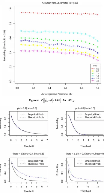
In this section we assess the reliability of our extreme value estimation method through a simulation study. This included a comparison between our estimation procedure and that of three alternative estima ion procedures for both the autocorrelation coefficient and the unknown location parameter under two different innovation distributions. Additionally, the degr of appr mation for the empirical probabilities of ˆmin
ee oxi
and ˆmin to its re
To study the pe the estimators
spective limiting distribution was reported. rformance of
min 1
1
t t
ˆ n Xt
X
ted 5000 replic bution at with index of regular variation and regular varying at 1 with a fixed index 1, whereas in case ii) the innovation distribution F2 is
regular varying at and with no restriction on or .
spectively, we genera ations for the non-
negative time series
X X0, 1, , Xn
r two differentsample sizes (500,1000), where
fo
tX is an AR(1)
process satisfying the difference equation
, for 1 and .
Xt Xt 1Zt t n Zt First we examine the simulation results for 0.9
under F1 for each of the six different values con-
sidered by computing 5000 estimates using
The autoregressive parameter is taken to be in the range from 0 to 1 guaranteeing a nonnegative time series and the unknown cation parameter lo is positive when
the innovations Zt min 1 max 1 range 1
1 1
ˆ n t ,ˆ t ,ˆ t j
t
t t t j
X X
X X
X X X X
∧
,are taken to
.
n let
ar
be
, if 1,
1 , if 1
c z z
F z
d z z
where t and j provides the index of the maximal and minimal Xi respectively for 1 i n, and
For this innovation distributio and d be non-
negative constants such that c d 1, then this dis- tribution is regularly varying at both endpoints with in- dex of regular v iation
c
at infinity and index of re-
gular variation at . For this simul
1
2 1
1 1
2 1
1 1
ˆ
,if 0 1
,if 1 3
LS
n n
t t t
t t
n n
t t t
t t
X X X
X X X X X X
ati udy two
distributions w onsi
on st
ere c dered:
1, 0, 1, ) 2, 0.5, 0.5.
F c d ii F c d
Now observe in case i) the innovation distribution 1
)
i where t1 t
n
X
X n. The means and standard de-viations (written below in parentheses), of these esti- mates are reported in Table 1 along with the average F
[image:10.595.65.536.392.737.2]is a Pareto distribution with a regular varying tail distri-
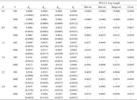
Table 1. Comparison of estimators for = 0.9 under F1.
95% C.I. Avg. Length
n
min ˆ
ˆmax ˆrange ˆLS Min est. Max est. Range est. LS est.
0.2 500 0.9000 0.9002 0.9002 0.8988 <0.0001 <0.0001 <0.0001 0.0288
(<0.0001) (0.0015) (0.0016) (0.0219) - - - -
1000 0.9000 0.9001 0.900