Explaining the Persistent Effect of Demand Uncertainty on Firm Growth

Munich Personal RePEc Archive

Explaining the Persistent Effect of

Demand Uncertainty on Firm Growth

Bricongne, Jean-Charles and Gigout, Timothee

Collège de France, Banque de France

1 May 2019

Online at

https://mpra.ub.uni-muenchen.de/97563/

Explaining the Persistent E

ff

ect of Demand

Uncertainty on Firm Growth

Jean-Charles Bricongne

_{Timothee Gigout}

May 30, 2019

Abstract

We study the effect of demand uncertainty on firm growth. We use product-level bi-lateral trade data to build an exogenous firm-level measure of the uncertainty of demand shocks. We match it with exhaustive custom and fiscal data between 1996 and 2013. An increase in uncertainty has a negative and persistent impact on the growth of exposed firms. This suggests a different underlying mechanism from a simple real-option effect. Financially constrained firms experience a much sharper and longer slowdown. Sectoral comovement is also a key factor explaining the persistent effect of uncertainty.

JEL classification:F23, D81, D22, F61

Keywords:Uncertainty; demand shock; Firm-level; Dynamics; Heterogeneity.

Acknowledgement: We thank participants of the 18th Doctoral Meetings in International

Trade and International Finance, the 2018 Meetings of the French Economic Associa-tion, the Banque de France PhD seminar and the 2018 CREA-IZA Workshop. In par-ticular, we are grateful to Clement Malgouyres, Antonin Bergeaud, Simon Ray, Matthieu Lequien, Nicolas Coeurdacier, Jose De Sousa, Gonzague Vannoorenberghe, Matthieu Bus-sière, Michel Beine and Thierry Mayer.

*_{Banque de France - Commission Européenne - Sciences-Po Paris, LIEPP - Université de Tours, LEO, Email:}

[email protected].

1

Introduction

The increase in cross-border trade and financial linkages since the 1990’s has led to a greater

exposure of domestic agents to shocks abroad. More firms are now dependent on inherently

uncertain demand conditions. In this paper, we investigate how the uncertainty around the

real-ization of demand shocks affects the growth dynamic of French manufacturing firms between

1996 and 2013. We build a measure of demand uncertainty by computing the dispersion of

estimated demand shocks from the highly dis-aggregated BACI bilateral trade database. We

then document the effect of an increase in demand uncertainty on employment and investment

growth using French fiscal data. A striking result is the persistent negative effect of a one-time

uncertainty shock. The effect lasts for up to 5 years for both investment and employment. It is

not followed by a period of compensation which makes those losses permanent. We find that

losses are magnified for financially constrained firms and firms with high correlation to their

industry.

The starting point of our paper is to compute a firm-level measure that captures the

uncer-tainty of demand shocks. Some studies use aggregate measures of unceruncer-tainty (Baker et al.

(2016),Julio and Yook(2012) orBussiere et al.(2015))). Others use stock market based

firm-level measures (Bloom et al.(2007), Barrero et al.(2017) orHassan et al.(2017)). We choose

instead to measure uncertainty using the firm exposure to the dispersion of estimated foreign

demand shocks. It has three distinct advantages. First, it allows us to focus on one properly

identified form of uncertainty, i.e. demand uncertainty. Second, it provides an exogenous

firm-level measure that we can causally link to the firm outcomes. Lastly, we obtain a wider and

more representative sample than one obtained using publicly listed firms.

To compute this measure, we follow a recent strand of literature relying on the computation

of foreign demand shocks. See Esposito(2018) for a review. Using the highly disagregated

database BACI (Gaulier and Zignago,2010), we first estimateproduct×exporting-country×

importing-country×yearidiosyncratic demand shocks. We then aggregate those shocks by

measuring their mean and dispersion at thesector×importing-country×yearlevel. We

use the dispersion as a proxy for uncertainty. Exports from France are excluded to prevent

en-dogeneity in the variations of those measures. To illustrate, the country-sector with the highest

demand uncertainty in our sample is the manufacture of coke and petroleum in Nigeria in 2010

which coincides with the death of the sitting president and the beginning of the first major terror

attacks by Boko Harram. We typically observe the highest values for other emerging countries

(Mali, Syria, Central African Republic) in raw material transformation sectors (manufacture of

wood, manufacture of other transport equipment, manufacture of paper, etc.). Finally, to obtain

a firm-level measure, we use a weighting scheme instrument as in Aghion et al. (2017) and

Mayer et al.(2016). We exploit differences in the firms’ initial exposures to the mean and

dis-persion of shocks associated with their own sector in any given importing country. The mean

represents the firm specific foreign demand, whereas the dispersion represents the firm specific

uncertainty of this demand.

We then regress several outcomes related to firm growth (Employment, investment, debt,

etc.) on this measure of uncertainty. We use Local Projections methods (Jordà,2005) to assess

the persistence of the effect a one time change in uncertainty. Local Projections have recently

been introduced for micro data where they provide a parsimonious and tractable alternative to

VAR models to compute impulse response functions in the presence of potential non-linearities

(seeFavara and Imbs(2015), Crouzet et al.(2017) and Cezar et al.(2017)). We find that

fol-lowing a one standard deviation increase in uncertainty, firms lower their investment growth

by -0.453 (s.e.= 0.114) percentage point and their employment growth by -0.581 (s.e.= 0.095)

percentage point. The negative effect lasts for 5 years for both investment and employment.

It does not exhibit any evidence of post-shock compensation (i.e. a positive value of the

co-efficient of uncertainty). Taken together, those results show that uncertainty has a permanent

negative effect on firm growth. Our key result contrasts with a central prediction from the

real-option theory. The value of the real-option of waiting should only temporally increase while there

is uncertainty about future outcomes. In this model, firms should then postpone investment

and compensate once the uncertainty is resolved (Bernanke,1983). We show that some of the

finan-cial frictions. However, even non finanfinan-cially constrained firms still experience a slight growth

slowdown. The ability to reverse the decision to scale up by selling the newly acquired

pro-duction capacity on a secondary is another candidate explanation. We also find that firms with

low irreversability (measured by the correlation of the firm with the sales of its industry) do

not suffer persistent effects from uncertainty. Whereas firms with high correlation experience a

much longer downturn.

A tangential benefit of our approach of using foreign demand shocks is to allow us to

mea-sure the effect of the transmission of uncertainty abroad on the growth of domestic firms. Our

study contributes to the debate of the effect of trade on firm dynamics. Many studies have now

documented the importance of idiosyncratic demand shocks to aggregate fluctuations. Garin

et al.(2017) investigate the impact of idiosyncratic foreign demand shocks on firm output and

workers individual wages. di Giovanni et al. (2017) show how idiosyncratic shock drives

ag-gregate fluctuations through large firms. Hummels et al.(2014) find that an exogeneous rise

in foreign demand increases employment and wages for both skilled and non skilled workers.

Other studies have focused on how idiosyncratic shock uncertainty affects exporters’ behavior.

It leads to lower than optimal size of supplier to allow for diversification (Gervais,2018). Only

large firms really benefit from diversification opportunities (Vannoorenberghe et al., 2016).

WhileEsposito(2018) shows that risk diversification leads to wellfare gains. Vannoorenberghe

(2012) shows that higher export share implies higher volatility of domestic sales. De Sousa

et al. (2016) find that expenditure uncertainty reduces exports. Especially, more productive

firms tend to abandon market shares in volatile destinations to less productive firms. Our study

complements those results by showing that losses caused by a 2nd _{moment shock (i.e. higher}

uncertainty) may potentially offset gains from a 1st _{moment shock (i.e. higher demand). We}

show that the uncertainty of demand has long lasting consequence for the growth of

manufac-turing firms. The failure to take into account demand uncertainty could lead to overestimating

gains from trade.

The reminder of the paper is organized as follows. Section 2 describes the data and our

methodology to compute the uncertainty of idiosyncratic demand shocks. Section3provides

our empirical results regarding the effect of uncertainty on firm growth. We show the robustness

of our results in Section4. Section5concludes.

2

Data

In the following subsections, we describe our data sources as well as the construction of our

variables of interest. We then provide some stylized facts concerning our new variables.

2.1

Data Sources

We build a database of matching fiscal, export and employment benefit data of French firms

between 1995 and 2013. We use export data from the French customs database to compute

firm-level exposure to foreign demand shocks and uncertainty. Firm accounting data come

from the French fiscal database FARE and FICUS. We use it to compute most of our control

(eg. productivity, cash flow, etc.) and dependent variables (investment, employment). It also

provides us with the firm primary sector of activity. Employee level data comes from the annual

social data declaration DADS. It allows us to decompose how firms arbitrage between

work-force size, structure and wages. It contains one observation per work contract with information

regarding the type of contract and various employee (age, gender, etc.) plus firm characteristics

(size, county, etc.). We calculate individual hourly wage growth rates then we average them

at the firm level. We use LIFI to control whether the firm belongs to a group. We use BACI

(Gaulier and Zignago, 2010) to compute import demand moments, including our uncertainty

proxy. BACI is a product-level bilateral trade database maintained by the CEPII. Finally, we

collect various country characteristics from the World Bank, the International Monetary Fund

and a few other ancillary sources. We present summary statistics in Table1. We follow about

Table 1:Firm characteristics

Outcome Variables Mean Std.Dev. P25 P50 P75

∆Capital_s,t 0.022 0.536 -0.156 -0.032 0.119

∆Tangible K_s,t 0.011 0.536 -0.196 -0.048 0.133

∆Intangible Ks,t 0.021 0.920 -0.141 0.000 0.048

∆Employment_s,t 0.086 0.346 0.000 0.051 0.167

∆White-collars_s,t 0.020 0.443 -0.105 0.000 0.167

∆Blue-collarss,t 0.005 0.417 -0.105 0.000 0.118

Control Variables

Log Total Assetss,t 15.040 1.735 13.835 14.876 16.064

Log Ks,t 12.658 2.111 11.302 12.575 13.947

Log Ls,t 3.241 1.385 2.303 3.135 4.007

Log Total Saless,t 15.101 1.667 13.959 14.964 16.097

Log Value Addeds,t 13.989 1.590 12.950 13.908 14.914

Log Productivitys,t 10.736 0.592 10.433 10.725 11.034

Log Debts,t 14.076 1.716 12.894 13.904 15.090

CashFlows,t

As,t−1 0.084 0.146 0.017 0.057 0.112

Leverages,t 1.762 3.361 0.387 0.728 1.453

Ages,t 21.723 13.820 11.000 19.000 31.000

♯Dests,t 9.686 14.140 1.000 4.000 12.000

ForeignS aless,t

T otalS aless,t 0.196 0.251 0.007 0.081 0.301

Variables of Interest

Demands,t 0.002 0.017 -0.000 0.000 0.002

Demand Uncertaintys,t 0.140 0.304 0.016 0.043 0.120

dDemand Uncertaintys,t 0.011 0.634 -0.104 -0.002 0.089

Observations 446590

NOTES: All outcome and control variables are computed using either fiscal (FARE, FICUS), social (DADS) or customs databases.

∆ Capitals,t is the log difference of the stock of non financial capital assets net of depreciation. ∆ Employments,t is the log difference of the number of employees (fiscal data). ∆Hourly Wages,t is the log difference of the firm average hourly wage. Log Productivitys,tis the log value added per worker. Log Ks,t is the log of tangible assets. Log Ls,t is measured in full-time equivalent workers at the end of the year. CashFlows,t

As,t−1 is the cash flow measured by operating income over lagged total assets. Leverages,t is the

leverage ratio measured by debt over equity. Log Debts,t is the log of total debt liabilities. Ages,t is in years.ForeignS aless,t

T otalS aless,t is the share of exports relative to total sales. ♯Dests,t is the number of foreign markets serviced by the firm. The variables of interest are computed using the bilateral product level database BACI. See Section2.2for the construction of the moments of the distribution of demand shocks. sandtindex firms

and years respectively..

2.2

Demand shocks and Uncertainty

The first step is to isolate demand shocks in the bilateral trade data. We follow a methodology

similar toGarin et al.(2017) andEsposito(2018). We have a set of countries J that import a

set of products Pfrom a set of countries I \ {i = FRA}. Let Vp,i,j,t be the imports of product

p from country i by country j in year t and ∆Vp,i,j,t be its log 1st difference. Then υp,i,j,t is

the idiosyncratic demand shock, computed as the residual of estimating the following equation

country by country:

∆Vp,i,j,t =β j

1∆Vp,i,t+β j

2∆Vp,j,t+α j j,t

| {z } Market Fundamentals

+ α_pj_,i,j

|{z}

Bilateral Product Trend

+υp,i,j,t

|{z}

Idiosyncratic Demand Shock

(1)

The intuition behind this 1st_{stage is the following}1_{. The fixed effectα}j

p,i,jremoves any bilateral

product trend that could generate increasing dispersion within an industry while being perfectly

"certain". For instance, it controls for heterogeneity between technologies: demand for old

products may decline relatively to new ones. The two aggregate growth rates can be thought

off as the market fundamentals on the demand and supply side for any particular year and

product. ∆Vp,j,t controls for the growth rate of imports of product pfrom the rest of the world

by country j. We are interested in the specific demand from j to i relative to that aggregate

fluctuation. All other things equal, the greater the residualυp,i,j,t, the more jwants pfromias

opposed to pfrom the rest of the worldI\ {i}. ∆Vp,i,t controls for the growth of exports ofiof

p to the rest of the world. All other things equal, if igets better at producing p, the residual

will be smaller. It therefore controls for supply shocks in i. The αj_j,t fixed effect controls for

aggregate conditions in the importing country jin yeart.

The residualsυp,i,j,t are by construction the variance that cannot be explained by either the

relevant trend or market fundamentals. Their first moment corresponds to the intensity of the

demand signal originating from that market. Their dispersion then tells us its noisiness, that

is how uncertain the signal would appear to an outside observer. We use this variable as our

time and country varying proxy for demand uncertainty. We compute the mean (DM1

k,j,t) for each

sector-import-year.Pp∈k,i,t is a counter for the number of non-zero trade flows in that triplet. Let

υ_kp_,j,t be the pth_{percentile of the distribution of allυ}

h,i,_FRAfor each sector-importer-year (k, j,t).

LetDM2

k,j,t be the 2

nd _{moment of the distribution of the idiosyncratic demand shocks of product}

pfrom sectorkin countryi(excluding France) into country j:

Mean: D_kM_,j1_,t = 1

Pp∈k,i,t−1

X

i,_FRA,p∈k

υp,j,i,t (2)

Dispersion: D_kM_,j2_,t = υ75_k,j,t−υ25_k,j,t (3)

This step provides robust and fairly intuitive measures of the shape of the distribution of demand

shocks. The higherDM1

k,j,t , the more intense the signal from that market. The higher the value

ofDM2

k,j,t, the wider the distribution and the nosier the signal. We compute alternative measures

using the spread betweenυ10_k,j,tandυ90_k,j,torυ5_k,j,tandυ95_k,j,tand confirm that our results are virtually

the same.

We now transform our sector-country-year measures into firm-year specific variables. We

follow the standard method in the literature (SeeAghion et al.(2017), Mayer et al.(2016) or

Berthou and Dhyne(2018)). We weight each of our demand distribution variable by the firm

initial market share and export intensity. The weights are necessary to account for the across

firms variations in market diversification. However by using the initial firm weights, we

en-sure that any across time fluctuations are only caused by variations of the demand distribution

measures and not by any endogenous firm reaction. In equation (4), we first weight our

sures on the initial share of country j in firm f export portfolio (Xj,f,t₀

Xf,t₀ ). We then average this

firm-destination level weighted variable across the export portfolio of firm f (Jf_{). Finally, we}

weight this measure over the initial export intensity of the firm (computed as Foreign Sales

(X∗

f,t0) over Total Sales (Y

∗ f,t0).

DM_f,t{1,2}= X ∗ f,t0 Y∗_f,t0

|{z}

1 Jf

! Jf

X

j=1

         

Xj,f,t0 Xf,t0

|{z}

D_kM₌{_k1,2}

f,j,t

         

Export Intensity Country Weight

(4)

2.3

Stylized Facts

Table2reports the 10 highest value of Demand Uncertainty in our sample. The country sector

with the highest value is the manufacture of coke and petroleum in Nigeria in 2010. It coincides

with the death of the sitting president and the beginning of the first major terror attacks by

Boko Harram. The next two values are Manufacture of other transport equipment in Iran 1997

(two massive earthquakes and a presidential election) and Rwanda 2010 (contested presidential

election). In Figure1, we plot the median value of the time series of each sector-by-country

panel. The color of the cell indicates the decile of uncertainty the country-sector belongs to.

Bright red indicates higher uncertainty and dark blue low uncertainty. Some countries like

Iran or Irak have a high demand uncertainty across most of their sectors while others like most

island nations have typically low demand uncertainty. Sectors like the machine manufacturing

industry (28), the car industry (29) and transport equipment industry (30) usually exhibit high

uncertainty across countries (SeeA.0.3for a list of all manufacturing sectors). There is however

plenty of variations within country or within sector.

In Figure2a, we plot the distribution of those idiosyncratic demand shocks for the car

p

Figure 1:Heatmap of the median value of demand uncertainty by sector and country

Afgha nist_an Al geri_a Andorra Angui lla Arge ntina Aruba Aust ria Baha mas Bangl ade_sh Bela_rus Beli_ze Berm_uda Bol ivia Bra zil Brune i Burki na Fa so Cam_bodi a Cana_da Caym an Isl ands Cha_d Chi_na Coc_{os Isl}

ands Com oros Cook Isl ands Cot e d'Ivoi re Cuba Cze_{ch R}

epubl ic De nm ark Dom inic_a Ecua_dor El Sa lva_dor Eritre_a Ethi_opi a Fiji Fra nce Ga_bon Ge orgi a Gha na Gre ece Gre nada Gua tem_ala Gui nea-B issa u Ha iti Hong Kong Iceland Indone sia Ira_q Isra el Jam aica Jorda n Ke_nya Kuwa it Laos Leba_non Libya Ma cao Ma daga scar Ma laysi a Ma li Ma rsha ll Isl ands Ma uri tius Mi crone sia Mongol ia Mont serra t Moz am bique Na_uru Ne the rlands Ne w C aledoni a Ni cara_gua Ni geri_a Nort h Kore a Om an Pa lau Pa nam_a Pa ragua y Phi lippi nes Port uga l Rom ani_a Rwa_nda Sa int Ki tts a nd Ne vis Sa int Pi erre and Mi que lon Sa moa Sa_{o T} om

e and Pri ncipe Se nega_l Sierra Leone Slova k R epubl ic Sol om on Isl ands Sout h Afri ca Sout h Suda n Sri Lanka Suri nam_e Swi tzerl_and Tajiki stan Tha iland Togo Trini dad a nd T oba go Turke y Turks a nd C aicos Isl ands Uga nda Uni ted Ara b E mira_tes Uni ted St ates Uz beki stan Ve nezue_la Wal_{lis a}

nd Fut una Yugosl avi_a Zim babwe Albani a Ameri can Sa moa Angol a Antigua and B arbuda Armeni a Austral ia Azerba ijan Bahra in Barba dos Belgi um Benin Bhut an Bosni a and He

rzegovi na

British Vi rgin Isl

ands Bulgari a Burundi Came roon Cape Ve

rde Centra l Afri can R epubl ic Chile Christm as Isl ands Colom bia Congo Costa R

ica Croa

tia Cyprus

Democ ratic R

epubl ic of C

ongo Djibout i Domini can R epubl ic Egypt Equa

torial Gui nea Estoni a Falkl and Isl ands Finland French Pol

ynesia Gambi a Germ any Gibra ltar Greenl and Guam Guinea Guya na Hondura s Hunga ry India Iran Ireland Italy Japan Kazakhst an Kiriba ti Kyrgyz Republ ic Latvi a Liberia Lithua nia Macedoni a Malawi Maldi ves Malta Mauri tania Mexic o Moldova Mont enegro Moroc co Myanm ar Nepal Nethe rlands Ant

illes New Z

ealNiand ger Niue Norwa y Pakist an Palest ine Papua New Gui

nea Peru Poland Qatar Russi a Saint Helena Saint Lucia Saint Vince

nt and t he Gre

nadines San Ma

rino Saudi Arabia Seyche lles Singa pore Slove nia Somali a South Kore

a Spain Suda n Sweden Syria Tanza nia Timor Tonga Tunisia Turkm enista n Tuva lu Ukra ine

United Ki ngdom Urugua y Vanua tu Vietna m Yeme n Zambi a

10 15 20 25 30

Sector (NAF 2-digit Code) 1 2 3 4 5 6 7 8 9 10

NOTE: See Section2.2for the construction method and the appendix for the description of the NAF sectors.

Table 2:Top 10 uncertain markets

D_kM_,2_j,t

1996 - Yemen - Manufacture of paper and paper products 9.62

1997 - Iran - Manufacture of other transport equipment 10.42

2002 - Cameroon - Manufacture of wood and of products of woo (...) 9.74

2003 - Central African Republic - Manufacture of other trans (...) 9.87

2007 - Equatorial Guinea - Manufacture of wood and of produc (...) 9.83

2009 - Vanuatu - Manufacture of other transport equipment 9.86

2010 - Nigeria - Manufacture of coke and refined petroleum p (...) 13.31

2010 - Rwanda - Manufacture of other transport equipment 10.17

2013 - Mali - Manufacture of wood and of products of wood an (...) 9.86

2013 - Syria - Manufacture of other transport equipment 10.14

in the USA and Germany mostly follows a normal shaped density function while it fluctuates

across time. Whereas demand from Columbia and China appears much noisier. We exploit

those time and geographical variations in the uncertainty of demand shocks to identify them.

Figure 2:Time-varying distribution of demand shocks for the car industry (1996-2015)

(a)3d density plot

Demand Shocks 1 25 De nsi ty 501996 2005 2015 4 5 6 USA Demand Shocks 1 25 De nsi ty 501996 2005 2015 4 5 6 DEU Demand Shocks 1 25 De nsi ty 501996 2005 2015 4 5 6 COL Demand Shocks 1 25 De nsi ty 501996 2005 2015 4 5 6 CHN

(b)Dispersion and Skewness

-.3 -.2 -.1 0 .1 .2 2 2.2 2.4 2.6 2.8 3

1995 2000 2005 2010 2015

USA -.3 -.2 -.1 0 .1 .2 2 2.2 2.4 2.6 2.8 3

1995 2000 2005 2010 2015

DEU -.3 -.2 -.1 0 .1 .2 2 2.2 2.4 2.6 2.8 3

1995 2000 2005 2010 2015

COL -.3 -.2 -.1 0 .1 .2 2 2.2 2.4 2.6 2.8 3

1995 2000 2005 2010 2015

CHN

Demand Uncertainty Idiosyncratic Demand Skewness

NOTE: Those figures show the time-varying shape of the distribution of demand shocks in the car industry for four countries. The left sub-figure presents the density for every duo-percentile of the distributions of demand shocks (eg. 25 is the median) for every year. The right sub-figure shows the 2nd and 3rd moment of the same distributions. See Section2.2for the construction method.

To illustrate our firm-level measure of demand uncertainty, Figure 3 plots the time series

of DM_f,t2 for three synthetic firms. We see that because of their different initial exposure to

foreign markets, each firm is experiencing a different evolution of demand uncertainty. Firm

Figure 3:Firm Level Demand Uncertainty 1996 1996 1996 1996 1996 1996 1996 1996 1996 1996 1997 1997 1997 1997 1997 1997 1997 1997 1997 1997 1998 1998 1998 1998 1998 1998 1998 1998 1998 1998 1999 1999 1999 1999 1999 1999 1999 1999 1999 1999 2000 2000 2000 2000 2000 2000 2000 2000 2000 20002001200120012001200120012001200120012001

2002 2002 2002 2002 2002 2002 2002 2002 2002 20022003200320032003200320032003200320032003

2004 2004 2004 2004 2004 2004 2004 2004 2004 2004 2005 2005 2005 2005 2005 2005 2005 2005 2005 2005 2006 2006 2006 2006 2006 2006 2006 2006 2006 2006 2007 2007 2007 2007 2007 2007 2007 2007 2007

2007200820082008200820082008200820082008_{200820092009201020092009200920092009200920092009}201020102010201020102010201020102010 2011 2011 2011 2011 2011 2011 2011 2011 2011 20112012201220122012201220122012201220122012

2013 2013 2013 2013 2013 2013 2013 2013 2013 20132014201420142014201420142014201420142014

1996 1996 1996 1996 1996 1996 1996 1996 1996 1996 1997 1997 1997 1997 1997 1997 1997 1997 1997 1997 1998 1998 1998 1998 1998 1998 1998 1998 1998 1998 1999 1999 1999 1999 1999 1999 1999 1999 1999 1999 2000 2000 2000 2000 2000 2000 2000 2000 2000 2000 2001 2001 2001 2001 2001 2001 2001 2001 2001

200120022002200220022002200220022002200220022003200320032003200320032003200320032003_{2004200420042004200420042004200420042004} 2005 2005 2005 2005 2005 2005 2005 2005 2005 20052006200620062006200620062006200620062006

2007 2007 2007 2007 2007 2007 2007 2007 2007 2007 2008 2008 2008 2008 2008 2008 2008 2008 2008 2008 2009 2009 2009 2009 2009 2009 2009 2009 2009 20092010201020102010201020102010201020102010

2011 2011 2011 2011 2011 2011 2011 2011 2011 20112012201220122012201220122012201220122012

2013 2013 2013 2013 2013 2013 2013 2013 2013 2013 2014 2014 2014 2014 2014 2014 2014 2014 2014 2014 1996 1996 1996 1996 1996 1996 1996 1996 1996 1996 1997 1997 1997 1997 1997 1997 1997 1997 1997 1997 1998 1998 1998 1998 1998 1998 1998 1998 1998 19981999199919991999199919991999199919991999

2000 2000 2000 2000 2000 2000 2000 2000 2000 20002001200120012001200120012001200120012001

2002 2002 2002 2002 2002 2002 2002 2002 2002 2002 2003 2003 2003 2003 2003 2003 2003 2003 2003 2003 2004 2004 2004 2004 2004 2004 2004 2004 2004 2004 2005 2005 2005 2005 2005 2005 2005 2005 2005

20052006200620062006200620062006200620062006_{20072007200820072007200720072007200720072007}2008200820092008200820082008200820082008200920092009200920092009200920092009 2010 2010 2010 2010 2010 2010 2010 2010 2010 2010 2011 2011 2011 2011 2011 2011 2011 2011 2011 2011 2012 2012 2012 2012 2012 2012 2012 2012 2012 201220132013201320132013201420132013201320132013201420142014201420142014201420142014

.05 .1 .15 .2

1995 2000 2005 2010 2015

Synthetic Firm n°1 (export intensity 1995 = 16.79%) Synthetic Firm n°2 (export intensity 1995 = 21.34%) Synthetic Firm n°3 (export intensity 1995 = 17.15%)

NOTE: This figure shows our firm-level measure of demand uncertainty (DM2_f,t) for three synthetic

firms. In order to satisfy anonymity requirements, each point is computed as the average value of uncertainty for 10 firms selected based on their closeness to the sample mean in terms of size and growth.

crisis. no_{2 then deals with high uncertainty throughout the entire period. Meanwhile, firm}

no1’s uncertainty returns to a more moderate level, with spikes around 2004, 2006 and 2013.

Whereas, firmno3 exhibits a much lower level of uncertainty as well as lower volatility.

3

Impact of Demand Uncertainty on Firm Growth

In this section, we first provide estimates of the firm growth path around an increase in demand

uncertainty using local projections. We then show how financial constraints and irreversibility

compound the effect of uncertainty.

3.1

Baseline Regressions

We use the Local Projections (LP) method as inJordà(2005) to recover the dynamic effect of

demand uncertainty on firm growth. We estimate its impact at up to 8 years after the initial

impulse and 6 years prior. Our variable of interest is the first simple difference of Demand

Uncertainty: dDM2

f,t. This variable has little correlation. We show the absence of

auto-correlation in FigureA.0.13for the same three synthetic firms as in Figure3. We confirm this

in a more generalized way with the Auto-Correlation Function in Figure A.0.14). The weak

auto-correlation dDM_f,t2 allows us to measure the effect of a one time increase in uncertainty.

Let:

Gf,t ={Capital,Employment}

then:

∆Gf,t+h =log

Gf,t+h

Gf,t−1

= αh

1Xf,t−1+αh2DMf,t1+β h

1dDMf,t2+γ

h k,t+γ

h

f +ǫf,t+h (5)

forh ∈ {−6,8}and where∆Gf,t+h denotes the cumulative change in outcome variableG from

time t to t + h. We use the log difference as in Bloom et al. (2007). We add a vector of

lagged controlsXf,t−1to capture relevant firm characteristics for investment (e.g. Gilchrist and

Himmelberg(1995),Bloom et al.(2007) andGala and Julio(2016)). By default, we include the

log ofGf,t−1, the lagged growth rate and level of foreign sales and the lagged level of demand

uncertainty (DM_f,t2₋₁). We also control for the current foreign demand signal (DM_f,t1). We add a

firm fixed effect to capture the time-invariant heterogeneity of firm dynamics. Finally, we add

a sector-time fixed effect to capture the sector business cycle. We cluster the standard errors at

the firm-level to account for potential within firm serial correlation in the error term (Bertrand

et al.,2004).

Figure4shows the effect of a one-standard deviation increase from the mean value ofdDM2

f,t

for investment and employment relative to the year before the shock. Both outcomes exhibit

little anticipatory response to the shock. On the left panel of Figure4, the impact on the stock

Figure 4: Demand Uncertainty and Firm Growth

(a)Investment

-0.09 0.05

-0.08 0.16 0.17

0.00

-0.45 -0.48 -0.22 -0.25

-0.31 0.02

-0.07 0.05

-0.20

-1 -.5 0 .5

-6 -4 -2 0 2 4 6 8

(b)Employment

0.01 0.11

0.06 0.09

0.05 0.00

-0.47 -0.39 -0.33

-0.19

-0.25 0.02

-0.03 -0.02

-0.11

-.6 -.4 -.2 0 .2 .4

-6 -4 -2 0 2 4 6 8

NOTE: Those figures present estimates of the coefficientβh

1∗100 associated with demand uncertainty from estimating this equation:∆Gf,t+h=αh₁Xf,t−1+αh₂DM1_f,t +βh₁dDM2_f,t +γh_k,t+γh_f+ǫf,t+h. 90%, 95% and 99% error

bands, computed with robust standard errors clustered at the firm-level, are displayed in shades of blue. The size of the shock is set at one standard deviation. E.g.: a one standard deviation uncertainty shock decreases investment growth by 0.45 percentage point the year of the shock.

However, only the first two years are significantly different from zero. It then reverts back to

approximately zero until the end of the eight-year window. A standard deviation size increase in

uncertainty results in a contemporaneous 0.45 percentage point lower growth rate of investment

(compared to a sample mean growth rate of 2.2%). Four years later, this increase still results in

a 0.31 p.p. lower growth rate. The effect on employment growth is negative until the fifth year

while it slowly reverts back to zero. It then remains at zero until the end of the time-window.

The contemporaneous effect is equal to 0.47 percentage point lower growth rate (compared to

a sample mean of 8.6% and an effect of -0.25 p.p. four years later).

Figure A.0.15presents the result from the same specification on other outcome variables.

The effect on tangible investment is stronger than the effect on intangible. The effect on debt

growth follows a very similar pattern as the effect on investment. We confirm the pattern and

magnitude of our result on employment by using data from the DADS social declarations rather

than from the fiscal declarations. We also find that the employment of white-collar workers is

somewhat more sensitive to uncertainty than the employment of blue-collar workers.

This persistent negative effect from a one time increase in uncertainty contrasts with the

wait-and-see effect predicted by the literature. We now examine two potential explanations. In

the next section, we show that this persistence is partially explained by firms facing financial

constraints prior to the shock. Then, we present results indicating that differences across firms

in the irreversibility of the growth decision is also driving some of the dynamic of the effect of

uncertainty.

3.2

Persistent E

_ff

ect of Uncertainty under Financial Constraint

As we are interested in how firm-level financial frictions may change the firm response to

uncertainty and explain the persistence of its effect, we interact our variable of interest with two

different measures indicating that the firm was financially constrained in the previous period.

The ability to generate cash-flow is a strong indicator of the ability to self-finance growth

or access external financing (Gala and Julio, 2016). Additionally, cash-flows can be used as

insurance against future shocks. The more financially constrained a firm is, the stronger and

more persistent its reaction to demand uncertainty should be. If a firm fears that drawing a

bad demand shock could lead to its default then its return on the option of waiting is higher. It

should therefore increase the effect of uncertainty. We estimate the following equation:

∆Gf,t+h =αh1Xf,t−1+αh2DMf,t1

+βh

1dDMf,t2+β h

2(dDMf,t2×CFf,t−1)+βh3CFf,t−1

+γh k,t+γ

h

f +ǫf,t+h

(6)

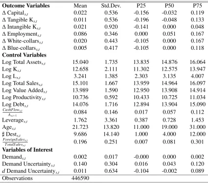
In Figure 5, we present the effect of demand uncertainty at various levels of the cash-flow

distribution. We use lagged cash-flow normalized over lagged assets trimmed at the 0.5 and

99.5 percentile. It excludes any observation where this measure is bellow -47% and above

46%. We then follow the methodology detailed byHainmueller et al. (2019). We allow the

coefficient βh

2 to vary across each quintiles of lagged cash-flow over assets. We then show

the effect of a standard deviation uncertainty shock estimated at the median of each quintile.

We focus once again on investment (first row) and employment (second row). The lower the

Figure 5:Demand Uncertainty and Cash Constraint High Low (a)Investment 0.00 -0.71 -0.75 -0.75 -1.18 -0.80 -0.53 -0.26 -3 -2 -1 0 1 2

0 2 4 6

Quintile n°1 0.00 -0.37 -0.62 -0.13 -0.44 -0.15 0.08 0.13 -3 -2 -1 0 1 2

0 2 4 6

Quintile n°2 0.00 -0.43 _-0.48 -0.04 0.19 -0.28 -0.47 _-0.55 -3 -2 -1 0 1 2

0 2 4 6

Quintile n°3 0.00 -0.56 -0.58 -0.34 -0.05 -0.12 0.03 0.05 -3 -2 -1 0 1 2

0 2 4 6

Quintile n°4 0.00 -0.49 -0.10 0.17 -0.03 0.04 0.48 0.39 -3 -2 -1 0 1 2

0 2 4 6

Quintile n°5 (b)Employment 0.00 -0.74 -0.90 -0.71 -0.24 -0.18 -0.19 0.07 -1.5 -1 -.5 0 .5 1

0 2 4 6

Quintile n°1 0.00 -0.11 0.04 -0.08 -0.08 0.12 0.32 0.30 -1.5 -1 -.5 0 .5 1

0 2 4 6

Quintile n°2 0.00 -0.16 -0.23 -0.03 0.28 -0.18 0.21 0.08 -1.5 -1 -.5 0 .5 1

0 2 4 6

Quintile n°3 0.00 _-0.04 0.14 0.31 0.49 0.44 0.41 0.20 -1.5 -1 -.5 0 .5 1

0 2 4 6

Quintile n°4 0.00 -0.37 -0.25 0.09 -0.02 -0.00 0.12 0.16 -1.5 -1 -.5 0 .5 1

0 2 4 6

Quintile n°5

NOTE: Those figure present estimates ofβh

2from estimating this equation:∆Gf,t+h=αh₁Xf,t−1+αh₂DM1_f,t+βh₁dDM2_f,t+βh₂(dDM2_f,t×CFf,t−1)+βh₃CFf,t−1+γkh,t+γ h

f+ǫf,t+h. 90%, 95% and 99% error bands, computed with robust standard errors clustered at the firm-level, are displayed in shades of blue.

When we allow the coefficients βh

2 to vary depending on the firm ability to generate

cash-flow, we find that the most financially constrained firms experience a somewhat sharper and

longer slowdown. The contemporaneous effect on investment is moderately bigger (0.71 vs

-0.49 p.p. for the bottom and top quintile respectively) Firms in the lowest quintile are still 1.18

percentage p.p. bellow their counter-factual investment growth rate 3 years after the shock.

Meanwhile, firms in the rest of the distributions are no longer suffering any effects. For

em-ployment growth, losses appear once again to be concentrated in the lowest quintile. The

contemporeneous effect is -0.74 p.p. for the 1st quintile versus approximately 0 for the next

three quintiles and -0.37 for the top quintile. Whereas the impact either reverts back to 0 or

turns positive for the top 4 quintiles, it remains negative for at least 3 periods for the bottom

bin of the cash-flow distribution.

The ability to generate cash flow only represents one facet of being financially constrained.

To investigate further, we repeat the same exercise for the firm’s stock of debt. We divide all

firms in 5 quintiles based on their ex-ante debt-to-asset ratio. We trim the ratio at the 99.5

percentile level. It excludes any observations with a ratio above 153% . We then estimate the

following equation:

∆Gf,t+h= αh1Xf,t−1+αh2DMf,t1

+βh

1dDMf,t2+β h

2(dDMf,t2×DAf,t−1)+βh3DAf,t−1

+γh k,t +γ

h

f +ǫf,t+h

(7)

and we plot the results in Figure6. The higher the quintile, the more financially constrained the

firm is. The investment of firms in the 1st two bins experiences a contemporaneous effect that

is lower than the sample average estimated earlier (-0.42 and -0.30 vs -0.45 p.p.) whereas firms

in the next three bins experience losses ranging from 0.66 to 0.86 percentage point. Moreover,

the investment of firms in the highest debt-to-asset bin has not recovered by the end of the

6-year window. The employment growth of firms in the lowest bin does not suffer. Firms in the

shock. Firms in the top two bins suffer severe losses (from -0.33 to -0.55 p.p.) for 2 to 3 years.

The effect then dies out in the following years unlike for investment.

Controlling for various forms of financial constraints does not reduce the estimated effect

of uncertainty by any substantive amount. However, the response to uncertainty does exhibit

strong non-linearity along either the debt or cash to asset ratio. The contemporaneous response

is usually barely distinguishable from zero for low constraints firms and does not exhibit any

persistence. Those results support the view that financial frictions are at least one of the reasons

behind the lack of a rebound effect expected after the resolution of an uncertainty shock.

Figure 6: Demand Uncertainty and Debt Constraint Low High (a)Investment 0.00 -0.42 -0.23 -0.49 -0.71 -0.30 _-0.35 -0.90 -2 -1 0 1 2

0 2 4 6

Quintile n°1 0.00 -0.30 -0.41 -0.22 0.00 -0.71 -0.35 0.59 -2 -1 0 1 2

0 2 4 6

Quintile n°2 0.00 -0.66 -0.67 0.41 -0.02 0.22 0.37 0.18 -2 -1 0 1 2

0 2 4 6

Quintile n°3 0.00 -0.76 -0.38 -0.53 -0.11 -0.42 0.06 0.03 -2 -1 0 1 2

0 2 4 6

Quintile n°4 0.00 -0.86 -0.94 -0.70 -0.92 -0.77 -0.63 -0.56 -2 -1 0 1 2

0 2 4 6

Quintile n°5 (b)Employment 0.00 -0.11 -0.03 0.11 -0.10 0.11 _0.20 0.33 -1 -.5 0 .5 1

0 2 4 6

Quintile n°1 0.00 -0.34 -0.21 -0.04 0.11 0.13 0.36 0.38 -1 -.5 0 .5 1

0 2 4 6

Quintile n°2 0.00 -0.57 -0.19 -0.19 0.08 0.07 0.09 0.21 -1 -.5 0 .5 1

0 2 4 6

Quintile n°3 0.00 -0.33 -0.43 -0.41 0.09 -0.11 0.24 -0.05 -1 -.5 0 .5 1

0 2 4 6

Quintile n°4 0.00 -0.47 -0.55 -0.14 -0.06 -0.24 -0.07 -0.24 -1 -.5 0 .5 1

0 2 4 6

Quintile n°5

NOTE: Those figures present estimates of from estimating this equation: M1 M2 ₍ M2 ₁₎

3.3

Sectoral Comovement and the Persistent E

_ff

ect of Uncertainty

Another potential explanation to the persistence of the effect of an uncertainty shock lies in the

degree of reversibility of the decision to grow. The more irreversible the decision to grow is,

the higher the return on the option of waiting and the stronger the initial impact of uncertainty

should be. Firms that are positively correlated with their sector will find it harder to sell or buy

on the secondary market. All firms in that sector are also more likely to face the same

uncer-tainty. Therefore no firms should be able to take advantage of this situation to acquire market

shares. In such a situation, an uncertainty shock may even trigger a sector-wide downturn. The

persistence of the estimated effect of the 2nd moment shock may include the 1st moment of

the second round effects. Firms with a negative correlation to their sector should benefit from

having a low option value when facing uncertainty. At the same time, their competitors are less

likely to face a similar uncertainty and should therefore be in a position to acquire market share

at the expanse of the uncertain. This mechanism should prevent firm-level uncertainty from

generating any aggregate fluctuations. Finally, firms that are neither positively or negatively

correlated with their sector are both benefiting from a low option value of waiting and little risk

of an uncertainty generated aggregate downturn.

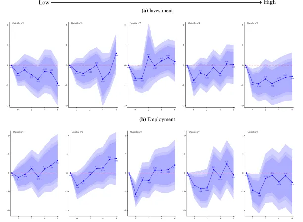
We followGuiso and Parigi (1999) to construct our measure of firm specific irreversibility

IRRf. We compute the correlation between the growth rate of the firm’s domestic sales and

the growth rate of the domestic sales of its industry. Formally, we compute for each firm-year

the average of the growth rate of sales for all other firms in the industry. Then, we compute

the pearson correlation coefficientIRRf = ρ(∆Yf,t,∆Ykf\f,t). This measure is bounded between

{−1,1}with 1 indicating a high irreversibility. As in the previous sections, we divide it in 5

quintiles and estimate the effect of uncertainty at the median of each quintile:

∆Gf,t+h =αh1Xf,t−1+αh2DMf,t1

+βh

1dDMf,t2+β h

2(dDMf,t2×IRRf)+βh3IRRf,t−1

+γh k,t+γ

h

f +ǫf,t+h

(8)

Our measure of irreversibility is not time-varying so its direct effect is absorbed by the firm fixed

effect. We plot the effect of its interaction with uncertainty in Figure7. Three striking results

emerge: (1) The investment and employment of firms with neither positive nor negative sectoral

co-movement (quintile no_{3) do not suffer much from an uncertainty shock, if anything they}

increase their employment in the longer run. (2) Firms with a negative correlation experience

a negative contemporaneous impact that quickly reverts back to zero. (3) Firms with high

sectoral correlation of their sales suffer from a more persistent slowdown. One explanation for

this would be that in a highly-correlated sector, the cost of drawing a bad demand shock would

be disproportionate as the firm would suspect that the other firms in the sector are drawing

similarly bad shocks. A rise in its uncertainty would make the firm cautious of the risk of a

sector-wide slowdown. In fact, if the other firms in the industry act in a similar fashion, it might

Figure 7:Demand Uncertainty and Sectoral Comovement

Negative Zero Positive

(a)Investment 0.00 -0.98 -0.55 -0.19 -0.58 -0.35 0.04 -0.17 -3 -2 -1 0 1 2

0 2 4 6

Quintile n°1 0.00 -0.58 -0.71 0.30 -0.68 -1.31 -0.56 -0.28 -3 -2 -1 0 1 2

0 2 4 6

Quintile n°2

0.00

-0.35 -0.38 -0.37 -0.21 -0.18 -0.35 -0.06 -3 -2 -1 0 1 2

0 2 4 6

Quintile n°3 0.00 -0.34 -0.80 -0.92 -0.54 -0.25 0.30 0.33 -3 -2 -1 0 1 2

0 2 4 6

Quintile n°4 0.00 -0.63 -0.54 -0.57 -0.57 -0.31 -0.15 -0.38 -3 -2 -1 0 1 2

0 2 4 6

Quintile n°5 (b)Employment 0.00 -0.56 -0.41 -0.28 0.23 0.05 0.52 0.28 -1 -.5 0 .5 1 1.5

0 2 4 6

Quintile n°1 0.00 -0.55 -0.40 _-0.30 -0.18 0.00 0.11 -0.07 -1 -.5 0 .5 1 1.5

0 2 4 6

Quintile n°2 0.00 -0.14 0.05 0.21 0.34 0.22 0.50 0.42 -1 -.5 0 .5 1 1.5

0 2 4 6

Quintile n°3 0.00 -0.29 -0.52 -0.38 _-0.41 -0.45 -0.12 0.05 -1 -.5 0 .5 1 1.5

0 2 4 6

Quintile n°4 0.00 -0.57 -0.49 -0.35 -0.42 -0.38 -0.28 -0.10 -1 -.5 0 .5 1 1.5

0 2 4 6

Quintile n°5

NOTE: Those figures present estimates ofβh

2from estimating this equation:∆Gf,t+h=αh₁Xf,t−1+αh₂DM1_f,t+βh₁dDM2_f,t+βh₂(dDM2_f,t×IRRf)+βh₃IRRf,t−1+γkh,t+γ h

f+ǫf,t+h. 90%, 95% and 99% error bands, computed with robust standard errors clustered at the firm-level, are displayed in shades of blue.

4

Robustness

4.1

Placebo Inference

In the baseline specification, we clustered standard errors at the firm level. This provided us

with standard errors that are asymptotically robust to serial auto-correlation in the error term.

Here we implementChetty et al.(2009)’s non-parametric permutation test2_ofβh>0

1 =0.

To do so, we randomly reassign the uncertainty time serie across firms and then we

re-estimate the baseline regression. We repeat this process 2000 times in order to obtain an

em-pirical distribution of the placebo coefficients ˆβh₁,p. If demand uncertainty had no effect on

firm growth, we would expect our baseline estimate to fall somewhere in the middle of the

distribution of the coefficients of the placebo coefficients ˆβh₁,p. Since that test does not rely

on any parametric assumption regarding the structure of the error term, it is immune to the

over-rejection of the null hypothesis highlighted byBertrand et al.(2004).

Figure 8: Distribution of Placebo Estimates

(a)Investment

-0.4 -0.2 0.0 0.2 0.4

-6 -4 -2 0 2 4 6 8

(b)Employment

-0.4 -0.2 0.0 0.2 0.4

-6 -4 -2 0 2 4 6 8

NOTE: Those figures present each half percentile of the distribution of 2000 estimates of the coefficient ˆβh₁,p

of Demand Uncertainty after performing a random permutation.

We plot the distribution of the placebo coefficients in Figure8. The figure confirms that our

coefficients of interestβh>0

1 (the blue connected markers) lie outside of the [p0.5,p99.5] interval

(the light blue lines) of the distribution of placebo coefficients. Meanwhile, the estimates of

βh<0

1 fall within the bounds of the distribution of placebos, albeit narrowly so in some cases.

This exercise confirms that uncertainty has a negative effect on firm growth.

4.2

Sensitivity

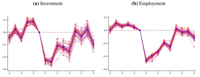
Since our sample includes events such as the Great Financial Crisis (2008 and 2009), we wish

to check whether our results are robust to the omission of any particular year. We run the same

baseline regressions while omitting turn by turn any year between 1996 and 2013. We plot the

results in Figure 10 in red. We find results that are quantitatively and qualitatively the same

as on the full sample. It shows that our specification satisfyingly accounts for the complex

dynamics of our sample period. We repeat this procedure for the sectors and plot the results

in purple in figure10. This estimate is also statistically highly significant and robust to taking

out any sectors (NAF 2 digit). Finally, we also demonstrate that this estimate is robust to the

inclusion of various observable characteristics in Figure9.

Figure 9:Sensitivity to sample selection

(a)Investment

-0.6 -0.4 -0.2 0.0 0.2

-6 -4 -2 0 2 4 6 8

(b)Employment

-0.6 -0.4 -0.2 0.0 0.2

-6 -4 -2 0 2 4 6 8

NOTE: Those figures present estimates of the coefficientβ₁of Demand Uncertainty after subtracting either a year or a sector at a time. We estimate the following equation:∆Gf,t+h=α1hXf,t−1+βh₁dDM2_f,t +γh_k,t+γh_f+ǫf,t+h.

4.3

Validation

To validate our measure of demand uncertainty, we check that an increase in demand has an

effect on firm growth. Given the existing literature on exports dynamics and productivity, we

Figure 10: Sensitivity to different specifications

(a)Investment

-0.60 -0.40 -0.20 0.00 0.20

-6 -4 -2 0 2 4 6 8

(b)Employment

-0.60 -0.40 -0.20 0.00 0.20

-6 -4 -2 0 2 4 6 8

NOTE: Those figures present estimates of the coefficientβ₁of Demand Uncertainty after adding one extra control variable at a time. We estimate the following equation:∆Gf,t+h=α₁hXf,t−1+βh₁dDM2_f,t+γ_kh_,t+γh_f+ǫf,t+h.

and add one of the following variable at a time: DM1_f,t, Lagged Cash-flow to asset ratio, a dummy variable

indicating whether the firm belongs to a group, lagged debt to asset ratio, lagged sales to asset ratio and lagged productivity.

suspect that the average firm’s response is not linear. We therefore regress firm capital and

employment growth on the 1st _{moment of foreign demand shocks interacted with lagged}

pro-ductivity (value-added over employees). We estimate the following equation:

Gf,t+h= αh1Xf,t−1+αh2DMf,t1+α h

3(DMf,t1×PRODf,t−1)+βh3PRODf,t−1+γh_k,t+γh_f +ǫf,t+h (9)

. We plot the results in Figure 11. The effect of a positive demand signal has little

short-run effect for investment. In the longer run (4 to 6 years), we see a sizable increase (about 1

percentage point per year for all terciles). The effect on employment is more contrasted. The

contemporaneous effect for firms in the lowest third of the productivity distribution is negative

(about 1/3rd of a p.p.). The effect then reverts back to zero and becomes positive in the next

3 years with a low statistical significance. The effect for the middle tercile is negative but

not significant for the first 2 years. It then becomes positive in the last 3 years. Firms with

the highest productivity increase their employment throughout the entire window. This result

matches the pattern highlighted byAghion et al.(2018). We therefore establish that firms react

Figure 11:Firm Growth, Foreign Demand Signal and Productivity

Low High

(a)Investment

-1 0 1 2 3

0 2 4 6

Tercile n°1

-1 0 1 2 3

0 2 4 6

Tercile n°2

-1 0 1 2 3

0 2 4 6

Tercile n°3

(b)Employment

-1 -.5 0 .5 1 1.5

0 2 4 6

Tercile n°1

-1 -.5 0 .5 1 1.5

0 2 4 6

Tercile n°2

-1 -.5 0 .5 1 1.5

0 2 4 6

Tercile n°3

NOTE: Those figures present estimates ofαh

3from estimating this equation:∆Gf,t+h=αh₁Xf,t−1+αh₂DM1_f,t+α₃h(DM1_f,t ×PRODf,t−1)+βh₃PRODf,t−1+γkh,t+γ h

f+ǫf,t+h. The 90% error band computed with robust standard errors clustered at the firm-level is displayed in blue.

5

Conclusion

The increase in cross-border trade and financial linkages since the 1990’s has led to a greater

exposure of domestic agents to shocks abroad. More firms are now dependent on inherently

uncertain demand conditions. In this paper, we investigate how the uncertainty around the

real-ization of demand shocks affects the growth dynamic of French manufacturing firms between

1996 and 2013. We build a measure of demand uncertainty by computing the dispersion of

esti-mated demand shocks from a highly dis-aggregated bilateral trade database. We then document

the effect of an increase in demand uncertainty on employment and investment growth using

French fiscal data. A striking result is the persistent negative effect of a one-time uncertainty

shock. The effect lasts for up to 5 years for both investment and employment. It does not

ex-hibit any evidence of post-shock compensation which makes those losses permanent. We find

that losses are magnified for financially constrained firms and firms with high sales correlation

with their sector.

Losses due to uncertainty are concentrated on the most financially constrained firms which

suggests that aggregate losses may be rather modest. However, our results show much more

persistent effect of uncertainty on the growth of firms than the temporary losses predicted by

the real-option theory. Policies that help reduce firm financial and information frictions would

therefore be an appropriate response to periods of high uncertainty by reducing permanent

losses among financially constrained firms, assuming those constraints are not correlated to

productivity. This implication seems particularly relevant given the current uncertainty around

A

Appendix

Figure A.0.12:Demand Signal to Noise

β = -0.014*** (s.e.= 0.005)

-5 0 5 10 De m and Unc ert ai nt y (st anda rdi ze d)

-10 -5 0 5 10 15

Demand Signal (standardized)

NOTE: This figure shows the correlation between the 1st and 2nd moment of the distribution of demand shocks. See Section2.2for the construction method.

Figure A.0.13:Firm Specific Demand Uncertainty - 1st difference

1997 1997 1997 1997 1997 1997 1997 1997 1997 1997 1998 1998 1998 1998 1998 1998 1998 1998 1998 1998 1999199919991999199919991999199919991999

2000 2000 2000 2000 2000 2000 2000 2000 2000 2000 2001 2001 2001 2001 2001 2001 2001 2001 2001 2001 2002 2002 2002 2002 2002 2002 2002 2002 2002 2002 2003 2003 2003 2003 2003 2003 2003 2003 2003 2003 2004 2004 2004 2004 2004 2004 2004 2004 2004 2004 2005 2005 2005 2005 2005 2005 2005 2005 2005 2005 2006 2006 2006 2006 2006 2006 2006 2006 2006 2006_{2007200720072007200720072007200720072007}

2008 2008 2008 2008 2008 2008 2008 2008 2008 2008 2009 2009 2009 2009 2009 2009 2009 2009 2009 2009 2010 2010 2010 2010 2010 2010 2010 2010 2010 2010 2011 2011 2011 2011 2011 2011 2011 2011 2011 2011 2012 2012 2012 2012 2012 2012 2012 2012 2012 2012 2013 2013 2013 2013 2013 2013 2013 2013 2013 2013 2014 2014 2014 2014 2014 2014 2014 2014 2014 2014 -.4 -.2 0 .2 .4

1995 2000 2005 2010 2015

Synthetic Firm n°1 (export intensity 1995 = 16.79%) Synthetic Firm n°2 (export intensity 1995 = 21.34%) Synthetic Firm n°3 (export intensity 1995 = 17.15%)

NOTE: This figures shows our firm-level measure of demand uncertainty (DM2_f,t) for three synthetic firms. In order to satisfy anonymity

Figure A.0.14: Demand Uncertainty Shock Local Projection

-.5 0 .5 1

-6 -4 -2 0 2 4 6 8

NOTE: This figure plots the coefficientsβh _{obtained from estimating the} local projection of the first difference of Demand Uncertainty dDM2_f,t+h =

βh_dDM2 f,t +γ

h k,t+γ

h

f +ǫf,t+h.

Figure A.0.15:Demand Uncertainty and Firm Growth (a)Debt 0.05 0.08 0.22 0.08 0.05 0.00 -0.47 -0.53 -0.37 -0.17 -0.24 -0.21 0.00 0.03 -0.10 -1 -.5 0 .5

-6 -4 -2 0 2 4 6 8

(b)Employment (Social Security sources)

-0.00 -0.06 -0.02 -0.13 -0.20 0.00 -0.58 -0.48 -0.36 -0.22 -0.17 0.08 -0.03 0.10 -0.01 -1 -.5 0 .5

-6 -4 -2 0 2 4 6 8

(c)White-collar -0.26 -0.18 -0.19 -0.07 -0.08 0.00

-0.40 _-0.45 -0.39 -0.13 0.08 -0.08 -0.28 -0.17 0.21 -1 -.5 0 .5 1

-6 -4 -2 0 2 4 6 8

(d)Blue-Collar

-0.07 -0.04

0.03 0.05 0.04 0.00

-0.40 -0.22 -0.26 -0.13 -0.16 0.04 -0.16 -0.10 -0.20 -1 -.5 0 .5

-6 -4 -2 0 2 4 6 8

(e)Tangible Investment

-0.19 0.04 -0.17 0.18 0.11 0.00 -0.54 -0.49 -0.44 -0.30 -0.12 0.13 -0.15 0.01 -0.03 -1 -.5 0 .5 1

-6 -4 -2 0 2 4 6 8

(f)Intangible Investment

0.41 0.48 -0.03 0.16 0.25 0.00 -0.50 -0.37 -0.16 -0.37 0.20 0.06 0.08 -0.36 0.01 -1.5 -1 -.5 0 .5 1

-6 -4 -2 0 2 4 6 8

NOTE: This figure presents estimates of the coefficientβh

1∗100 associated with demand uncertainty from estimating this equation:∆Gf,t+h=αh₁Xf,t−1+αh₂DM1_f,t +βh₁dDM2_f,t +γh_k,t+γh_f+ǫf,t+h. 90%, 95% and 99% error

Table A.0.3: List of Sectors

10 Manufacture of food products

11 Manufacture of beverages

12 Manufacture of tobacco products

13 Manufacture of textiles

14 Manufacture of wearing apparel

15 Manufacture of leather and related products

16 Manufacture of wood and of products of wood and cork, except furniture;

manufacture of articles of straw and plaiting materials

17 Manufacture of paper and paper products

18 Printing and reproduction of recorded media

19 Manufacture of coke and refined petroleum products

20 Manufacture of chemicals and chemical products

21 Manufacture of basic pharmaceutical products and pharmaceutical preparations

22 Manufacture of rubber and plastic products

23 Manufacture of other non-metallic mineral products

24 Manufacture of basic metals

25 Manufacture of fabricated metal products, except machinery and equipment

26 Manufacture of computer, electronic and optical products

27 Manufacture of electrical equipment

28 Manufacture of machinery and equipment n.e.c.

29 Manufacture of motor vehicles, trailers and semi-trailers

30 Manufacture of other transport equipment

31 Manufacture of furniture

32 Other manufacturing

References

Aghion, P., A. Bergeaud, M. Lequien, and M. Melitz (2017). The Impact of Exports on

Inno-vation: Theory and Evidence. Technical report, working paper.

Aghion, P., A. Bergeaud, M. Lequien, and M. J. Melitz (2018). The impact of exports on

innovation: Theory and evidence. Technical report, National Bureau of Economic Research.

Baker, S. R., N. Bloom, and S. J. Davis (2016). Measuring economic policy uncertainty. The

Quarterly Journal of Economics 131(4), 1593–1636.

Barrero, J. M., N. Bloom, and I. Wright (2017). Short and long run uncertainty. Technical

report, National Bureau of Economic Research.

Bernanke, B. S. (1983). Irreversibility, uncertainty, and cyclical investment. The Quarterly

Journal of Economics 98(1), 85–106.

Berthou, A. and E. Dhyne (2018). Exchange Rate Movements, Firm-Level Exports and

Het-erogeneity.

Bertrand, M., E. Duflo, and S. Mullainathan (2004). How much should we trust diff

erences-in-differences estimates? The Quarterly journal of economics 119(1), 249–275.

Bloom, N., S. Bond, and J. Van Reenen (2007). Uncertainty and Investment Dynamics. The

review of economic studies 74(2), 391–415.

Bussiere, M., L. Ferrara, and J. Milovich (2015). Explaining the Recent Slump in Investment:

The Role of Expected Demand and Uncertainty. Technical report, Banque de France

Work-ing Paper.

Cezar, R., T. Gigout, and F. Tripier (2017). FDI and Uncertainty: Evidence from French

Multinational Firms. Technical report, Working Paper.

Chetty, R., A. Looney, and K. Kroft (2009). Salience and taxation: Theory and evidence.

Crouzet, N., N. R. Mehrotra, et al. (2017). Small and Large Firms Over the Business Cycle.

Technical report.

De Sousa, J., A.-C. Disdier, and C. Gaigné (2016). Export decision under risk.

di Giovanni, J., A. A. Levchenko, and I. Mejean (2017). Large firms and international business

cycle comovement. American Economic Review 107(5), 598–602.

Esposito, F. (2018). Entrepreneurial Risk and Diversification through Trade.

Favara, G. and J. Imbs (2015). Credit supply and the price of housing. American Economic

Review 105(3), 958–92.

Gala, V. and B. Julio (2016). Firm Size and Corporate Investment.

Garin, A., F. Silverio, et al. (2017). How Does Firm Performance Affect Wages? Evidence

from Idiosyncratic Export Shocks. Technical report, Job Market Papers.

Gaulier, G. and S. Zignago (2010). BACI: international trade database at the product-level (the

1994-2007 version).

Gervais, A. (2018). Uncertainty, risk aversion and international trade. Journal of International

Economics 115, 145–158.

Gilchrist, S. and C. P. Himmelberg (1995). Evidence on the role of cash flow for investment.

Journal of Monetary Economics 36(3), 541–572.

Guiso, L. and G. Parigi (1999). Investment and demand uncertainty. The Quarterly Journal of

Economics 114(1), 185–227.

Hainmueller, J., J. Mummolo, and Y. Xu (2019). How much should we trust estimates from

multiplicative interaction models? Simple tools to improve empirical practice. Political

Analysis 27(2), 163–192.

Hassan, T. A., S. Hollander, L. van Lent, and A. Tahoun (2017). Firm-level political risk:

Measurement and effects. Technical report, National Bureau of Economic Research.

Hummels, D., R. Jørgensen, J. Munch, and C. Xiang (2014). The wage effects of offshoring:

Evidence from danish matched worker-firm data.American Economic Review 104(6), 1597–

1629.

Jordà, Ò. (2005). Estimation and inference of impulse responses by local projections.American

Economic Review 95(1), 161–182.

Julio, B. and Y. Yook (2012). Political uncertainty and corporate investment cycles.The Journal

of Finance 67(1), 45–83.

Khwaja, A. I. and A. Mian (2008). Tracing the impact of bank liquidity shocks: Evidence from

an emerging market. American Economic Review 98(4), 1413–42.

Mayer, T., M. J. Melitz, and G. I. Ottaviano (2016). Product mix and firm productivity

re-sponses to trade competition. Technical report, National Bureau of Economic Research.

Vannoorenberghe, G. (2012). Firm-level volatility and exports. Journal of International

Eco-nomics 86(1), 57–67.

Vannoorenberghe, G., Z. Wang, and Z. Yu (2016). Volatility and diversification of exports: