On the Effects of the BRICS on World Economic Growth

Munich Personal RePEc Archive

On the Effects of the BRICS on World

Economic Growth

Bosupeng, Mpho

University of Botswana

2017

On the Effects of the BRICS on World

Economic Growth

Author: Mpho Bosupeng

Email: [email protected]

This is the Accepted Version!

FINAL VERSION IS HERE:

On the Effects of the BRICS on World Economic Growth

Abstract

The purpose of this empirical study is to examine the potential effects of the BRICS on other economies’ economic growth over the period 1960-2013. This investigation deploys the

Saikkonen and L tkepohl cointegration methodology to validate long run relations between u

Brazil and China’s economic growth and other nation’s output growth. The study further uses the Toda and Yamamoto approach to Granger causality to examine long run causal links between the BRICS economic growth. The results show that all countries exhibit long run relations with China and Brazil’s economic growth. In addition, the results prove that Brazil’s economic growth is induced by South Africa, China and India’s economic growth.

Introduction

The acronym BRICS refers to a set of fast developing nations namely: Brazil, Russia, India, China and South Africa. Economic growth exhibited by these economics has been quite impressive in the last decades particularly for China and India. China’s economic growth has been exponential over the years. Today China is the second largest economy in the world. Additionally China’s influence has been robust in matters such as exports variety, carbon dioxide emissions, global sustainable development and skills transfer in many economies. Exponential economic growth is desirable but it has shortcomings. For instance the BRICS are currently concerned with reducing emissions without hampering economic prosperity. China is currently the largest emitter of carbon dioxide globally. India also registered the highest emissions growth recently. Nonetheless, the BRICS are leading world economic growth.

The common aspect among the BRICS is that they are industrialised exporters. Economists postulated that countries such as China and India are a clear example of the export-led growth hypothesis. Export-led growth economies rely heavily on exports to drive sectors of the economy. Mineral exporting economies such as South Africa have to consider the prudent use of their resources and economic development. Over the years many economies have relied on the BRICS for their imports. Numerous studies have been examined to investigate the influence of the BRICS in matters such as inflation spillovers and market returns. Sustainable development is desirable however countries need to cooperate for this endeavour to be realised. An economy cannot be self-sufficient in all sectors.

The question is how does economic growth of the BRICS affect a given economy? How do the BRICS interact in their attempts to reach sustainable development? This paper aims to answer all these questions. This study focuses on Brazil and China to determine the long run effects of these economies’ growth on other nations. The reason for focusing on China and Brazil are follows. China is currently the second largest economy and her global influence has multiplied. Brazil is also highly influential in South America. The other reason is geographical location. Brazil is located far west while China is in Asia. This is important to determine global influence of these economies without being biased to Asian economies only such as Russia, India and China. The second aim is to investigate the causal relations between members of the BRICS’s economic growth patterns. The reason for this aim is that the BRICS need to depend on each other in various sectors for their own sustainable development. In this way their global influence will be prodigious (synergy).

In this paper the cointegration method proposed by Saikkonen and L tkepohl (2000) as well u

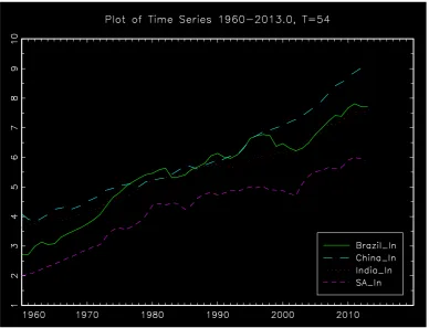
Figure 1: Progress of Economic Growth (1960-2013)

Note: The data has been converted to natural logarithms so that it is easy to monitor the volatility of the variables over the material period. Due to data unavailability Russia was not included in this analysis. Source: JMulti (4) statistical package.

Literature Review

Studies pertaining to economic growth have been numerous. Chang et al (2013) examined the effects of exports and globalization on economic growth using the corrected least square variable model for five South Caucasus countries (Azerbaijan, Armenia, Georgia, Russia and Turkey). The results of the study revealed that exports with higher energy content and globalization induce economic growth. Amador (2012) highlighted that the BRICS members Brazil, India and China possess high energy content in manufacturing exports. The authors noted that economic growth is dependent on other factors such as political and social integration. The results of this study are conceivable because political turmoil tends to disrupt economic growth in many economics especially in Africa. The problem with high energy content exports is the production of emissions in the manufacturing process. Carbon dioxide is not the only gas we should be concerned about. Sulphur dioxide is also a challenge and has detrimental effects on the environment and people. Chang et al (2013) argued that energy exports and globalisation are important determinants of economic prosperity in the South Caucasus region.

the results revealed that the real appreciation of the Rupee adversely affects India’s exports performance. Under this circumstance, economic growth is also affected because output depends on the positivity of net exports. As the Rupee appreciates, Indian exports become more expensive to importing economies thus registering a decline in demand. Tekin (2012) examined causation between real GDP, real exports and Foreign Domestic Investment (FDI) in least developed countries over the period 1970 to 2009.The results demonstrated that exports induce economic growth in Haiti, Rwanda and Sierra Leone. Such countries can be termed as export-led growth economies. Export export-led growth economies have to consider how they can reduce emissions without hampering economic growth. Economic growth was found to accelerate exports growth of the following economies: Angola, Chad and Zambia. FDI was found to Granger cause GDP in Benin and Togo.

A summary of the reviewed literature shows that economic growth is affected by several factors such as exchange rates, political and social integration. The BRICS are associated with high energy exports following (Amador, 2012). This study intends to determine the influence of the BRICS on other economies’ economic growth over the period 1960 to 2013. The investigation applies the recent cointegration method proposed by Saikkonen and L tkepohl (2000). The u

examination further uses the Toda and Yamamoto (1995) approach to determine the direction of causation between economic growths among the BRICS.

Materials and Methods

This study examines the relations between GDP for sixty different economies with the BRICS over the period 1960 to 2013. The data was obtained from a web source named The Global

Economy (http://www.theglobaleconomy.com/). Russia was not included in this analysis due

to absence of material data. Actual GDP was in billion dollars (U$). The actual data was converted to natural logarithms before proceeding with empirical analysis. The reason is technically, it is easier to monitor the volatility of logarithmic values over the material period as compared to using raw data. It is imperative that the data set is examined for unit roots. The Augmented Dickey Fuller test (see Dickey and Fuller, 1979) was selected to test for stationarity of the variables. The testing procedure of the ADF is derived from the following generalized model:

∆𝑦𝑡=𝛼+𝛽𝑡+𝛾𝑦𝑡 ‒1+𝛿∆𝑦𝑡 ‒1+⋯+𝛿𝑝 ‒1∆𝑦𝑡 ‒ 𝑝+ 1+𝜀𝑡,

The model applied in this study is:

∴ ∆𝑦𝑡=𝛼+𝛽𝑡+𝛾𝑦𝑡 ‒1+

𝑘

∑

𝑖= 1

𝛿𝑖∆𝑦𝑡 ‒1+ 𝜀𝑡.

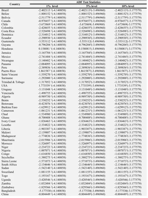
Table 1: Augmented Dickey Fuller (ADF) Test Results

ADF Test Statistics Country

1% level 5% level 10% level

Brazil -2.402113 1_{(-4.140858) -2.402113}2_{(-3.496960) -2.402113}3_(-3.177579)

Belize -1.808152 1_{(-4.140858) -1.808152}2_{(-3.496960) -1.808152}3_(-3.177579)

Bolivia -2.511779 1_{(-4.140858) -2.511779}2_{(-3.496960) -2.511779}3_(-3.177579)

Canada -0.978457 1_{(-4.140858) -0.978457}2_{(-3.496960) -0.978457}3_(-3.177579)

Chile -3.673869 1_{(-4.140858) -3.673869(-3.496960) -3.673869(-3.177579)}

Colombia -2.428655 1_{(-4.140858) -2.428655}2_{(-3.496960) -2.428655}3_(-3.177579)

Costa Rica -2.528498 1_{(-4.140858) -2.528498}2_{(-3.496960) -2.528498}3_(-3.177579)

Dominica -2.316012 1_{(-4.140858) -2.316012}2_{(-3.496960) -2.316012}3_(-3.177579)

Ecuador -2.290930 1_{(-4.140858) -2.290930}2_{(-3.496960) -2.290930}3_(-3.177579)

Guatemala -3.553112 1_{(-4.140858) -3.553112(-3.496960) -3.553112(-3.177579)}

Guyana -0.796204 1_{(-4.140858) -0.796204}2_{(-3.496960) -0.796204}3_(-3.177579)

Honduras 0.158081 1_{(-4.140858) 0.158081}2_{(-3.496960) 0.158081}3_(-3.177579)

Jamaica -3.165784 1_{(-4.140858) -3.165784}2_{(-3.496960) -3.165784}3_(-3.177579)

Mexico -2.741484 1_{(-4.140858) -2.741484}2_{(-3.496960) -2.741484}3_(-3.177579)

Nicaragua -3.140482 1_{(-4.140858) -3.140482}2_{(-3.496960) -3.140482}3_(-3.177579)

Panama -2.084095 1_{(-4.140858) -2.084095}2_{(-3.496960) -2.084095}3_(-3.177579)

Peru -2.389856 1_{(-4.140858) -2.389856}2_{(-3.496960) -2.389856}3_(-3.177579)

Puerto Rico 1.861587 1_{(-4.140858) 1.861587}2_{(-3.496960) 1.861587}3_(-3.177579)

Saint Vincent -1.559270 1_{(-4.140858) -1.559270}2_{(-3.496960) -1.559270}3_(-3.177579)

Suriname -1.292000 1_{(-4.140858) -1.292000}2_{(-3.496960) -1.292000}3_(-3.177579)

Trinidad & Tobago -1.317052 1_{(-4.140858) -1.317052}2_{(-3.496960) -1.317052}3_(-3.177579)

USA 1.773539 1_{(-4.140858) 1.773539}2_{(-3.496960) 1.773539}3_(-3.177579)

Uruguay -3.131048 1_{(-4.140858) -3.131048}2_{(-3.496960) -3.131048}3_(-3.177579)

Venezuela -1.498755 1_{(-4.140858) -1.498755}2_{(-3.496960) -1.498755}3_(-3.177579)

Algeria -0.989750 1_{(-4.140858) -0.989750}2_{(-3.496960) -0.989750}3_(-3.177579)

Benin -2.530252 1_{(-4.140858) -2.530252}2_{(-3.496960) -2.530252}3_(-3.177579)

Botswana -0.423076 1_{(-4.140858) -0.423076}2_{(-3.496960) -0.423076}3_(-3.177579)

Burkina Faso -1.629912 1_{(-4.140858) -1.629912}2_{(-3.496960) -1.629912}3_(-3.177579)

Cameroon -1.061231 1_{(-4.140858) -1.061231}2_{(-3.496960) -1.061231}3_(-3.177579)

Chad -1.534980 1_{(-4.140858) -1.534980}2_{(-3.496960) -1.534980}3_(-3.177579)

Ghana -0.700408 1_{(-4.140858) -0.700408}2_{(-3.496960) -0.700408}3_(-3.177579)

Ivory Coast -1.836463 1_{(-4.140858) -1.836463}2_{(-3.496960) -1.836463}3_(-3.177579)

Lesotho -2.334822 1_{(-4.140858) -2.334822}2_{(-3.496960) -2.334822}3_(-3.177579)

Liberia -1.903387 1_{(-4.140858) -1.903387}2_{(-3.496960) -1.903387}3_(-3.177579)

Malawi -2.139807 1_{(-4.140858) -2.139807}2_{(-3.496960) -2.139807}3_(-3.177579)

Madagascar -1.774836 1_{(-4.140858) -1.774836}2_{(-3.496960) -1.774836}3_(-3.177579)

Mauritania -2.015906 1_{(-4.140858) -2.015906}2_{(-3.496960) -2.015906}3_(-3.177579)

Morocco -1.526097 1_{(-4.140858) -1.526097}2_{(-3.496960) -1.526097}3_(-3.177579)

Niger -2.234723 1_{(-4.140858) -2.234723}2_{(-3.496960) -2.234723}3_(-3.177579)

Nigeria -1.007071 1_{(-4.140858) -1.007071}2_{(-3.496960) -1.007071}3_(-3.177579)

Congo -1.616850 1_{(-4.140858) -1.616850}2_{(-3.496960) -1.616850}3_(-3.177579)

Seychelles -1.380275 1_{(-4.140858) -1.380275}2_{(-3.496960) -1.380275}3_(-3.177579)

Sierra Leone -1.571073 1_{(-4.140858) -1.571073}2_{(-3.496960) -1.571073}3_(-3.177579)

South Africa -2.134646 1_{(-4.140858) -2.134646}2_{(-3.496960) -2.134646}3_(-3.177579)

Sudan -1.542140 1_{(-4.140858) -1.542140}2_{(-3.496960) -1.542140}3_(-3.177579)

Swaziland -1.881155 1_{(-4.140858) -1.881155}2_{(-3.496960) -1.881155}3_(-3.177579)

Togo -1.193167 1_{(-4.140858) -1.193167}2_{(-3.496960) -1.193167}3_(-3.177579)

Uganda -3.420546 1_{(-4.140858) -3.420546}2_{(-3.496960) -3.420546(-3.177579)}

Zambia -1.032484 1_{(-4.140858) -1.032484}2_{(-3.496960) -1.032484}3_(-3.177579)

Zimbabwe -1.829366 1_{(-4.140858) -1.829366}2_{(-3.496960) -1.829366}3_(-3.177579)

Hong Kong -0.593099 1_{(-4.140858) -0.593099}2_{(-3.496960) -0.593099}3_(-3.177579)

India -1.686225 1_{(-4.140858) -1.686225}2_{(-3.496960) -1.686225}3_(-3.177579)

Israel -1.830077 1_{(-4.140858) -1.830077}2_{(-3.496960) -1.830077}3_(-3.177579)

Japan -0.125997 1_{(-4.140858) -0.125997}2_{(-3.496960) -0.125997}3_(-3.177579)

Malaysia -1.651926 1_{(-4.140858) -1.651926}2_{(-3.496960) -1.651926}3_(-3.177579)

Nepal -2.366434 1_{(-4.140858) -2.366434}2_{(-3.496960) -2.366434}3_(-3.177579)

Oman -1.219531 1_{(-4.140858) -1.219531}2_{(-3.496960) -1.219531}3_(-3.177579)

Pakistan -2.469553 1_{(-4.140858) -2.469553}2_{(-3.496960) -2.469553}3_(-3.177579)

The ADF test statistics are reported above. The critical values are as follows: -[4.140858] is the critical value at 1% level; -[3.496960] is the critical value at 5% level and -[3.177579] is the critical value at 10% level.The numbers in brackets are critical values. Superscripts 1, 2, 3 indicate statistical significance at 1%, 5%, and 10% critical levels. The results are based on the model: ∆𝑦𝑡=𝛼+𝛽𝑡+𝛾𝑦𝑡 ‒1+∑𝑘_{𝑖= 1}𝛿𝑖∆𝑦𝑡 ‒1+ 𝜀𝑡. Eviews 7 was used to compute the ADF unit root test. The null hypothesis for the test is “series x, has a unit root”.

Saikkonen and L tkepohl (2000) Cointegration Model𝑢

In this study, it is important to examine the long run relations between the series. This paper applies the recent cointegration method proposed by Saikkonen and L tkepohl (2000). u

Cointegrated variables will be attracted to each other therefore resulting in long run affiliations. Even though the Johansen cointegration test and the Saikkonen and L tkepohl test are almost u

similar, there are technical differences. Firstly, the Saikkonen and L tkepohl test is different u

technically because it estimates the deterministic term first and then subtracts it from the time

series observations unlike the Johansen method. Saikkonen and L tkepohl (2000) commenced u

their model by considering a 𝑉𝐴𝑅(𝑝) process of the form:

𝑦𝑡=𝑣+𝐴1𝑦𝑡 ‒1+⋯+𝐴𝑝𝑦𝑡 ‒ 𝑝+𝜀𝑡 𝑡=𝑝+ 1,𝑝+ 2,…,

Following Saikkonen and L tkepohl (2000) allow to be u 𝐴_𝐽 𝑛×𝑛 coefficient matrices while 𝜀_𝑡 is an 𝑛× 1 is a stochastic error term assumed to be a martingale difference sequence with𝐸

. The non-stochastic positive definite conditional covariance matrix was

(

│

)

defined as𝐸

(

│

)

∆𝑦𝑡=𝑣+Π𝑦𝑡 ‒1+

𝑝 ‒1

∑

𝑗= 1

Γ𝑗∆𝑦𝑡 ‒ 𝑗+𝜀𝑡 𝑡=𝑝+ 1,𝑝+ 2,…,

The definition of terms is Π=‒

(

)

(

)

. The test validates if .

The Toda and Yamamoto (1995) Approach to Granger Causality

The aim of this paper is to investigate the long run causation between income series. However, in this study the other challenge is determining the direction of causal affiliations between income series of the BRICS. The Toda and Yamamoto (1995) approach is the most suitable because it does not require pre-tests for cointegration. The Granger causality test (see Granger, 1969) was not selected because not all data in this study is non-stationary (Bangladesh income series was stationary). The Toda and Yamamoto (1995) technique can apply even if the series does not have unit roots. Granger causality also has several limitations. Originally, if the variables under consideration are driven by a common third process with different lags, there is a possibility of failing to reject the alternative hypothesis of Granger causality. In addition, Granger causality is often based on the assumption that causal relations are a result of cointegration. The advantage of the Toda and Yamamoto (1995) approach is that the VAR’s formulated in the levels can be estimated even if the processes may be integrated or cointegrated of an arbitrary order. Wolde-Rufael (2005) observed that the Toda and Yamamoto (1995) approach fits a standard vector autoregressive model in the levels of the variables. In consequence, this minimizes risks associated with the likelihood of wrongly identifying the order of integration of the series (Mavrotas and Kelly, 2001).

The literature has developed a number of cointegration methods following the contributions of Saikkonen and L tkepohl (2000); Johansen and Juselius (1990); Johansen (1988b, 1991a); u Granger (1981); Granger and Weiss (1983); Engle and Granger (1987); Granger and Engle (1985); Stock (1987); Phillips and Durlauf (1986); Phillips and Park (1986); Phillips and Ouilaris (1986); Stock and Watson (1987); Park (1992a, 1990b); Phillips and Hansen (1990); Hovarth and Watson (1995); Saikkonen (1992) and Elliot (1998). Toda and Yamamoto (1995) noted that if economic variables are not cointegrated then the VAR should be estimated in first– order differences of the variables to validate the conventional asymptotic theory. In consequence, the Toda and Yamamoto (1995) approach is applicable even if the VAR may be stationary, integrated of an arbitrary order or cointegrated of an arbitrary order.

This study applies the Toda and Yamamoto (1995) approach as discussed by Wolde-Rufael

(2005). The testing procedure starts by augmenting the correct VAR order by the maximal 𝑘

order of integration _𝑑 (Wolde-Rufael, 2005). Following this, a th _{order of the}

𝑚𝑎𝑥 (𝑘+𝑑𝑚𝑎𝑥)

VAR is estimated and the coefficients of the last lagged 𝑑_𝑚𝑎𝑥 vector are ignored (Caporale and Pittis, 1999; Rambaldi and Doran, 1996; Rambaldi, 1997; Zapata and Rambaldi, 1997).

Denote two income series as LX and LY. The VAR system of the variables can now be shown

as:

𝐿𝑋𝑡=𝛼0+

𝑘

∑

𝑖= 1

𝛼1𝑖𝐿𝑋𝑡 ‒ 𝑖+

𝑑𝑚𝑎𝑥

∑

𝑗=𝑘+ 1

𝛼2𝑗𝐿𝑋𝑡 ‒ 𝑗+

𝑘

∑

𝑖= 1

∅1𝑖𝐿𝑌𝑡 ‒ 𝑖+

𝑑𝑚𝑎𝑥

∑

𝑗=𝑘+ 1

∅2𝑗𝐿𝑌𝑡 ‒ 𝑗+𝜆1𝑡

𝐿𝑌𝑡=𝛽0+

𝑘

∑

𝑖= 1

𝛽1𝑖𝐿𝑌𝑡 ‒1+

𝑑𝑚𝑎𝑥

∑

𝑗=𝑘+ 1

𝛽2𝑗𝐿𝑌𝑡 ‒ 𝑗+

𝑘

∑

𝑖= 1

𝛿1𝑖𝐿𝑋𝑡 ‒ 𝑖+

𝑑𝑚𝑎𝑥

∑

𝑗=𝑘+ 1

Empirical Results

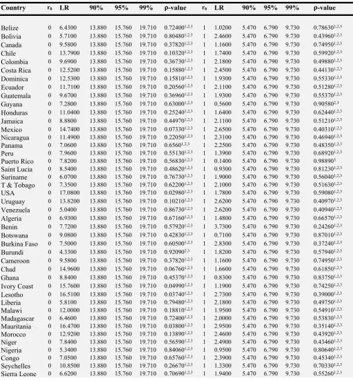
The Saikkonen and L tkepohl test was carried out at 90%, 95% and 99% critical levels using u

JMulti (4) statistical package. The results show that there is a long run relationship between all the countries’ economic growth and the two countries income (Brazil and China). Tables 2 and 3 represent the results of the cointegration test. Note that -values less than the critical levels ρ of 90%, 95% and 99% represent cointegration.

Table 2: Results of the Saikkonen and L tkepohl Cointegration Test (Brazil)𝐮

Country r0 LR 90% 95% 99% 𝛒-value r0 LR 90% 95% 99% 𝛒-value

Belize 0 6.4300 13.880 15.760 19.710 0.724001,2,3 _{1 1.0200 5.470 6.790 9.730 0.78630}1,2,3

Bolivia 0 5.7100 13.880 15.760 19.710 0.804801,2,3 _{1 2.4600 5.470 6.790 9.730 0.43960}1,2,3

Canada 0 9.5800 13.880 15.760 19.710 0.378201,2,3 _{1 1.1600 5.470 6.790 9.730 0.74950}1,2,3

Chile 0 13.7900 13.880 15.760 19.710 0.103201,2,3 _{1 1.7400 5.470 6.790 9.730 0.59920}1,2,3

Colombia 0 9.6900 13.880 15.760 19.710 0.367301,2,3 _{1 2.1800 5.470 6.790 9.730 0.49880}1,2,3

Costa Rica 0 12.5200 13.880 15.760 19.710 0.158801,2,3 _{1 2.4500 5.470 6.790 9.730 0.44130}1,2,3

Dominica 0 12.5300 13.880 15.760 19.710 0.158101,2,3 _{1 1.9300 5.470 6.790 9.730 0.55330}1,2,3

Ecuador 0 11.7100 13.880 15.760 19.710 0.205601,2,3 _{1 2.1100 5.470 6.790 9.730 0.51280}1,2,3

Guatemala 0 9.6700 13.880 15.760 19.710 0.369601,2,3 _{1 1.9300 5.470 6.790 9.730 0.55370}1,2,3

Guyana 0 7.2800 13.880 15.760 19.710 0.630001,2,3 _{1 0.5600 5.470 6.790 9.730 0.90580}2,3

Honduras 0 11.0400 13.880 15.760 19.710 0.252401,2,3 _{1 1.6400 5.470 6.790 9.730 0.62440}1,2,3

Jamaica 0 8.8800 13.880 15.760 19.710 0.449701,2,3 _{1 2.1100 5.470 6.790 9.730 0.51210}1,2,3

Mexico 0 14.7400 13.880 15.760 19.710 0.073301,2,3 _{1 2.6500 5.470 6.790 9.730 0.40310}1,2,3

Nicaragua 0 11.4900 13.880 15.760 19.710 0.220501,2,3 _{1 2.3100 5.470 6.790 9.730 0.46940}1,2,3

Panama 0 7.0600 13.880 15.760 19.710 0.65601,2,3 _{1 2.2500 5.470 6.790 9.730 0.48350}1,2,3

Peru 0 7.9600 13.880 15.760 19.710 0.551301,2,3 _{1 1.3900 5.470 6.790 9.730 0.68920}1,2,3

Puerto Rico 0 7.8200 13.880 15.760 19.710 0.568301,2,3 _{1 0.1400 5.470 6.790 9.730 0.98890}3

Saint Lucia 0 8.5400 13.880 15.760 19.710 0.486201,2,3 _{1 0.9300 5.470 6.790 9.730 0.81230}1,2,3

Suriname 0 6.0700 13.880 15.760 19.710 0.767301,2,3 _{1 1.9000 5.470 6.790 9.730 0.56040}1,2,3

T & Tobago 0 7.3500 13.880 15.760 19.710 0.622001,2,3 _{1 2.1000 5.470 6.790 9.730 0.51630}1,2,3

USA 0 17.0800 13.880 15.760 19.710 0.029801,2,3 _{1 1.7800 5.470 6.790 9.730 0.59080}1,2,3

Uruguay 0 13.8200 13.880 15.760 19.710 0.102101,2,3 _{1 2.6200 5.470 6.790 9.730 0.40970}1,2,3

Venezuela 0 5.0400 13.880 15.760 19.710 0.867301,2,3 _{1 2.6200 5.470 6.790 9.730 0.40940}1,2,3

Algeria 0 6.9300 13.880 15.760 19.710 0.671601,2,3 _{1 1.4800 5.470 6.790 9.730 0.66570}1,2,3

Benin 0 7.7200 13.880 15.760 19.710 0.579201,2,3 _{1 3.7300 5.470 6.790 9.730 0.24260}1,2,3

Botswana 0 9.0800 13.880 15.760 19.710 0.428301,2,3 _{1 0.7100 5.470 6.790 9.730 0.87010}1,2,3

Burkina Faso 0 7.5000 13.880 15.760 19.710 0.605001,2,3 _{1 2.8300 5.470 6.790 9.730 0.37240}1,2,3

Burundi 0 4.3300 13.880 15.760 19.710 0.920902,3 _{1 1.8200 5.470 6.790 9.730 0.57940}1,2,3

Cameroon 0 9.5800 13.880 15.760 19.710 0.378201,2,3 _{1 1.1600 5.470 6.790 9.730 0.74950}1,2,3

Chad 0 14.9600 13.880 15.760 19.710 0.067601,2,3 _{1 1.6600 5.470 6.790 9.730 0.61850}1,2,3

Ghana 0 8.8400 13.880 15.760 19.710 0.453701,2,3 _{1 0.8300 5.470 6.790 9.730 0.83750}1,2,3

Ivory Coast 0 15.7600 13.880 15.760 19.710 0.049901,2,3 _{1 1.1900 5.470 6.790 9.730 0.74250}1,2,3

Lesotho 0 16.5100 13.880 15.760 19.710 0.037401,2,3 _{1 2.7300 5.470 6.790 9.730 0.39000}1,2,3

Liberia 0 5.8100 13.880 15.760 19.710 0.794801,2,3 _{1 2.1800 5.470 6.790 9.730 0.49750}1,2,3

Malawi 0 12.0000 13.880 15.760 19.710 0.188101,2,3 _{1 1.9500 5.470 6.790 9.730 0.54910}1,2,3

Madagascar 0 6.4600 13.880 15.760 19.710 0.724001,2,3 _{1 2.0000 5.470 6.790 9.730 0.53830}1,2,3

Mauritania 0 16.4700 13.880 15.760 19.710 0.038001,2,3 _{1 2.9500 5.470 6.790 9.730 0.35140}1,2,3

Morocco 0 12.9200 13.880 15.760 19.710 0.138901,2,3 _{1 2.4600 5.470 6.790 9.730 0.43920}1,2,3

Niger 0 7.8400 13.880 15.760 19.710 0.565901,2,3 _{1 2.4900 5.470 6.790 9.730 0.43460}1,2,3

Nigeria 0 5.3400 13.880 15.760 19.710 0.840601,2,3 _{1 0.9500 5.470 6.790 9.730 0.80640}1,2,3

Congo 0 7.0500 13.880 15.760 19.710 0.657601,2,3 _{1 2.3900 5.470 6.790 9.730 0.45340}1,2,3

Seychelles 0 10.8500 13.880 15.760 19.710 0.266701,2,3 _{1 1.3300 5.470 6.790 9.730 0.70330}1,2,3

Note:1 _{shows statistical significance at 90% critical level;} 2 _{shows statistical significance at 95% critical level;} 3_{shows statistical}

significance at 99% critical level. Note that -values less than critical levels of 90%, 95% and 99% represent cointegration. ρ The test was carried out using JMulti 4 statistical package. The deterministic term of the VECM was defined as 𝐷_𝑡=𝑢_𝑜+𝑢_1𝑡. Superscripts 1, 2, 3 show statistical significance at 90%, 95%, and 99% critical levels. LR = Likelihood Ratio. Superscripts 1, 2, 3 show statistical significance at 90%, 95%, and 99% critical levels.

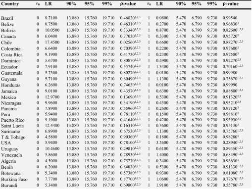
Table 3: Results of the Saikkonen and L tkepohl Cointegration Test (China)𝐮

South Africa 0 13.1100 13.880 15.760 19.710 0.130301,2,3 _{1 1.7300 5.470 6.790 9.730 0.60280}1,2,3

Sudan 0 6.0600 13.880 15.760 19.710 0.767701,2,3 _{1 2.5200 5.470 6.790 9.730 0.42890}1,2,3

Swaziland 0 10.8900 13.880 15.760 19.710 0.263401,2,3 _{1 1.8400 5.470 6.790 9.730 0.57600}1,2,3

Togo 0 16.2100 13.880 15.760 19.710 0.042101,2,3 _{1 2.7100 5.470 6.790 9.730 0.39380}1,2,3

Uganda 0 13.5300 13.880 15.760 19.710 0.113001,2,3 _{1 2.4000 5.470 6.790 9.730 0.45230}1,2,3

Zambia 0 8.5800 13.880 15.760 19.710 0.481601,2,3 _{1 0.9600 5.470 6.790 9.730 0.80180}1,2,3

Zimbabwe 0 10.3600 13.880 15.760 19.710 0.306501,2,3 _{1 2.4400 5.470 6.790 9.730 0.44440}1,2,3

Bangladesh 0 15.0900 13.880 15.760 19.710 0.064301,2,3 _{1 2.3200 5.470 6.790 9.730 0.46850}1,2,3

China 0 8.7100 13.880 15.760 19.710 0.468201,2,3 _{1 0.0800 5.470 6.790 9.730 0.99540}

Hong Kong 0 13.6300 13.880 15.760 19.710 0.109201,2,3 _{1 1.1700 5.470 6.790 9.730 0.74560}1,2,3

India 0 7.3600 13.880 15.760 19.710 0.621301,2,3 _{1 1.2300 5.470 6.790 9.730 0.73040}1,2,3

Israel 0 8.3500 13.880 15.760 19.710 0.507901,2,3 _{1 1.1300 5.470 6.790 9.730 0.75690}1,2,3

Japan 0 8.1500 13.880 15.760 19.710 0.529601,2,3 _{1 0.3400 5.470 6.790 9.730 0.95630}3

Malaysia 0 11.3400 13.880 15.760 19.710 0.230801,2,3 _{1 1.3200 5.470 6.790 9.730 0.70730}1,2,3

Nepal 0 7.6500 13.880 15.760 19.710 0.587201,2,3 _{1 2.3100 5.470 6.790 9.730 0.47130}1,2,3

Oman 0 12.7800 13.880 15.760 19.710 0.145701,2,3 _{1 0.7700 5.470 6.790 9.730 0.85270}1,2,3

Pakistan 0 13.2300 13.880 15.760 19.710 0.125001,2,3 _{1 2.6600 5.470 6.790 9.730 0.40140}1,2,3

Country r0 LR 90% 95% 99% 𝛒-value r0 LR 90% 95% 99% 𝛒-value

Brazil 0 8.7100 13.880 15.760 19.710 0.468201,2,3 _{1 0.0800 5.470 6.790 9.730 0.99540}

Belize 0 8.7500 13.880 15.760 19.710 0.463101,2,3 _{1 0.2700 5.470 6.790 9.730 0.96830}3

Bolivia 0 10.0500 13.880 15.760 19.710 0.333401,2,3 _{1 0.8700 5.470 6.790 9.730 0.82600}1,2,3

Canada 0 6.0400 13.880 15.760 19.710 0.770301,2,3 _{1 0.3300 5.470 6.790 9.730 0.95720}3

Chile 0 17.4500 13.880 15.760 19.710 0.025601,2,3 _{1 0.6600 5.470 6.790 9.730 0.88270}1,2,3

Colombia 0 6.6400 13.880 15.760 19.710 0.703901,2,3 _{1 0.2200 5.470 6.790 9.730 0.97680}3

Costa Rica 0 9.1900 13.880 15.760 19.710 0.417301,2,3 _{1 0.2300 5.470 6.790 9.730 0.97500}3

Dominica 0 5.6700 13.880 15.760 19.710 0.808701,2,3 _{1 0.4900 5.470 6.790 9.730 0.92270}2,3

Ecuador 0 7.9100 13.880 15.760 19.710 0.557401,2,3 _{1 1.3400 5.470 6.790 9.730 0.70160}1,2,3

Guatemala 0 5.7300 13.880 15.760 19.710 0.802701,2,3 _{1 0.0100 5.470 6.790 9.730 0.99980}

Guyana 0 5.7100 13.880 15.760 19.710 0.804901,2,3 _{1 1.1300 5.470 6.790 9.730 0.75670}1,2,3

Honduras 0 6.2600 13.880 15.760 19.710 0.746301,2,3 _{1 0.0100 5.470 6.790 9.730 0.99990}

Jamaica 0 9.0100 13.880 15.760 19.710 0.435701,2,3 _{1 0.6300 5.470 6.790 9.730 0.88800}1,2,3

Mexico 0 12.9700 13.880 15.760 19.710 0.136901,2,3 _{1 0.5300 5.470 6.790 9.730 0.91320}2,3

Nicaragua 0 9.9600 13.880 15.760 19.710 0.341901,2,3 _{1 0.4500 5.470 6.790 9.730 0.93210}2,3

Panama 0 7.8900 13.880 15.760 19.710 0.559601,2,3 _{1 0.2600 5.470 6.790 9.730 0.97120}3

Peru 0 5.9400 13.880 15.760 19.710 0.781101,2,3 _{1 0.1500 5.470 6.790 9.730 0.98810}3

Puerto Rico 0 9.1900 13.880 15.760 19.710 0.416401,2,3 _{1 0.4200 5.470 6.790 9.730 0.93930}2,3

Saint Lucia 0 12.4400 13.880 15.760 19.710 0.163101,2,3 _{1 0.3600 5.470 6.790 9.730 0.95130}3

Suriname 0 6.8900 13.880 15.760 19.710 0.675301,2,3 _{1 1.1300 5.470 6.790 9.730 0.75760}1,2,3

T & Tobago 0 4.5800 13.880 15.760 19.710 0.903602,3 _{1 0.1800 5.470 6.790 9.730 0.98280}3

USA 0 5.9400 13.880 15.760 19.710 0.781001,2,3 _{1 3.3600 5.470 6.790 9.730 0.28940}1,2,3

Uruguay 0 10.4600 13.880 15.760 19.710 0.298101,2,3 _{1 0.6100 5.470 6.790 9.730 0.89350}1,2,3

Venezuela 0 5.8600 13.880 15.760 19.710 0.789301,2,3 _{1 1.4000 5.470 6.790 9.730 0.68490}1,2,3

Algeria 0 4.5000 13.880 15.760 19.710 0.752701,2,3 _{1 0.3400 5.470 6.790 9.730 0.95630}3

Benin 0 6.2000 13.880 15.760 19.710 0.840301,2,3 _{1 0.5300 5.470 6.790 9.730 0.91330}1,2,3

Botswana 0 5.3400 13.880 15.760 19.710 0.573801,2,3 _{1 0.9300 5.470 6.790 9.730 0.81080}1,2,3

Burkina Faso 0 7.7700 13.880 15.760 19.710 0.877001,2,3 _{1 1.0600 5.470 6.790 9.730 0.77670}1,2,3

Note:1 _{shows statistical significance at 90% critical level;} 2 _{shows statistical significance at 95% critical level;} 3_{shows statistical}

significance at 99% critical level. Note that -values less than critical levels of 90%, 95% and 99% represent cointegration. ρ The test was carried out using JMulti 4 statistical package. The deterministic term of the VECM was defined as 𝐷_𝑡=𝑢_𝑜+𝑢_1𝑡. Superscripts 1, 2, 3 show statistical significance at 90%, 95%, and 99% critical levels. LR = Likelihood Ratio.

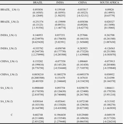
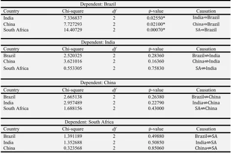
Eviews 7 was used to carry out the Toda and Yamamoto (1995) approach to causality. The results show that Brazil’s income is induced by China, South Africa and India’s economic growth. The countries registered -values less than the 5% critical level suggesting that we ρ have to reject the null hypothesis of non-causality. Table 4 is a presentation of the VAR estimates before the causality test. Table 5 presents the results of the Toda and Yamamoto (1995) causality test.

Cameroon 0 4.9200 13.880 15.760 19.710 0.740501,2,3 _{1 0.5900 5.470 6.790 9.730 0.89980}1,2,3

Chad 0 6.6900 13.880 15.760 19.710 0.692701,2,3 _{1 0.5700 5.470 6.790 9.730 0.90390}2,3

Ghana 0 6.3200 13.880 15.760 19.710 0.740501,2,3 _{1 0.6500 5.470 6.790 9.730 0.88340}1,2,3

Ivory Coast 0 6.7400 13.880 15.760 19.710 0.692701,2,3 _{1 1.8400 5.470 6.790 9.730 0.57630}1,2,3

Lesotho 0 7.5400 13.880 15.760 19.710 0.600701,2,3 _{1 0.5600 5.470 6.790 9.730 0.90740}2,3

Liberia 0 11.0600 13.880 15.760 19.710 0.250401,2,3 _{1 0.7000 5.470 6.790 9.730 0.87090}1,2,3

Malawi 0 9.0400 13.880 15.760 19.710 0.432501,2,3 _{1 0.4100 5.470 6.790 9.730 0.94000}2,3

Madagascar 0 5.0100 13.880 15.760 19.710 0.869401,2,3 _{1 2.0600 5.470 6.790 9.730 0.52490}1,2,3

Mauritania 0 6.2500 13.880 15.760 19.710 0.747701,2,3 _{1 1.1000 5.470 6.790 9.730 0.76630}1,2,3

Morocco 0 6.7800 13.880 15.760 19.710 0.688701,2,3 _{1 0.0600 5.470 6.790 9.730 0.99710}

Niger 0 7.9200 13.880 15.760 19.710 0.556701,2,3 _{1 0.6300 5.470 6.790 9.730 0.88870}1,2,3

Nigeria 0 6.4900 13.880 15.760 19.710 0.721701,2,3 _{1 1.5800 5.470 6.790 9.730 0.64020}1,2,3

Congo 0 8.2200 13.880 15.760 19.710 0.521501,2,3 _{1 2.4200 5.470 6.790 9.730 0.44840}1,2,3

Seychelles 0 8.1700 13.880 15.760 19.710 0.527401,2,3 _{1 0.6100 5.470 6.790 9.730 0.89520}1,2,3

Sierra Leone 0 8.5500 13.880 15.760 19.710 0.485601,2,3 _{1 1.6100 5.470 6.790 9.730 0.63200}1,2,3

South Africa 0 7.9700 13.880 15.760 19.710 0.550801,2,3 _{1 0.4700 5.470 6.790 9.730 0.92660}2,3

Sudan 0 6.3500 13.880 15.760 19.710 0.737001,2,3 _{1 0.2800 5.470 6.790 9.730 0.96690}3

Swaziland 0 8.8100 13.880 15.760 19.710 0.456901,2,3 _{1 0.5900 5.470 6.790 9.730 0.89900}1,2,3

Togo 0 8.0500 13.880 15.760 19.710 0.541801,2,3 _{1 0.5100 5.470 6.790 9.730 0.91750}2,3

Uganda 0 14.9200 13.880 15.760 19.710 0.068601,2,3 _{1 0.6000 5.470 6.790 9.730 0.89650}1,2,3

Zambia 0 7.0000 13.880 15.760 19.710 0.662701,2,3 _{1 0.6900 5.470 6.790 9.730 0.87340}1,2,3

Zimbabwe 0 9.9500 13.880 15.760 19.710 0.343001,2,3 _{1 0.1300 5.470 6.790 9.730 0.98990}3

Bangladesh 0 19.9800 13.880 15.760 19.710 0.008901,2,3 _{1 0.5400 5.470 6.790 9.730 0.91110}2,3

Hong Kong 0 7.2300 13.880 15.760 19.710 0.636701,2,3 _{1 1.7200 5.470 6.790 9.730 0.60530}1,2,3

India 0 6.0100 13.880 15.760 19.710 0.773701,2,3 _{1 0.4900 5.470 6.790 9.730 0.92320}2,3

Israel 0 6.5400 13.880 15.760 19.710 0.715201,2,3 _{1 0.4300 5.470 6.790 9.730 0.93640}2,3

Japan 0 8.5700 13.880 15.760 19.710 0.483401,2,3 _{1 0.4600 5.470 6.790 9.730 0.92920}2,3

Malaysia 0 5.3800 13.880 15.760 19.710 0.836101,2,3 _{1 0.6600 5.470 6.790 9.730 0.88220}1,2,3

Nepal 0 13.3600 13.880 15.760 19.710 0.119901,2,3 _{1 0.8800 5.470 6.790 9.730 0.82530}1,2,3

Oman 0 6.5800 13.880 15.760 19.710 0.710501,2,3 _{1 0.0300 5.470 6.790 9.730 0.99890}3

Table 4: Vector Autoregression (VAR) Estimates

BRAZIL INDIA CHINA SOUTH AFRICA

BRAZIL_ LN(-1) 0.893856 0.159168 -0.053817 0.09826 (0.14585) (0.10593) (0.10323) (0.14993) [6.12849] [1.50255] [-0.52131] [0.65779]

BRAZIL_LN(-2) -0.251374 -0.139890 -0.058306 0.020327 (0.13123) (0.09531) (0.09288) (0.13490) [-1.91556] [-1.46774] [-0.62774] [0.15068]

INDIA_LN(-1) 0.146953 0.857351 0.257046 0.262708 (0.234970) (0.170650) (0.166310) (0.241540) [0.625420] [5.02391] [1.545600] [1.087630]

INDIA_LN(-2) -0.555782 -0.050748 0.283923 -0.126563 (0.244730) (0.177750) (0.173220) (0.251580) [-2.270990] [-0.285500] [-1.639080] [-0.503070]

CHINA_LN(-1) 0.155202 -0.077558 1.090469 -0.073913 (0.199810) (0.145120) (0.141430) (0.205400) [0.776750] [-0.534440] [7.710570] [-0.359840]

CHINA_LN(-2) 0.0838210 0.1885270 -0.0493370 0.030952 (0.2085500) 0.151470 0.147610 0.214390 [0.401920 [1.244660] [-0.334230] [0.144370]

SA_LN(-1) 0.4900440 0.093754 0.0298370 1.066611 (0.174350) (0.126630) (0.123400) (0.179230) [2.810750] [0.740400] [0.241780] [5.951210]

SA_LN(-2) 0.030164 -0.055641 0.1072180 -0.313102 (0.183150) (0.133020) (0.129630) (0.188270) [0.164700] [-0.418300] [0.827100] [-1.663030]

Table 5: Toda and Yamamoto Causality Test Results

Dependent: Brazil

Country Chi-square df ρ-value Causation

India 7.336837 2 0.02550* India⇒Brazil

China 7.727293 2 0.02100* China⇒Brazil

South Africa 14.40729 2 0.00070* SA⇒Brazil

Dependent: India

Country Chi-square df ρ-value Causation

Brazil 2.520325 2 0.28360 Brazil⇎India

China 3.621016 2 0.16360 China⇎India

South Africa 0.553305 2 0.75830 SA⇎India

Dependent: China

Country Chi-square df ρ-value Causation

Brazil 2.665138 2 0.26380 Brazil⇎China

India 2.957489 2 0.22790 India⇎China

South Africa 1.688156 2 0.43000 SA⇎China

Dependent: South Africa

Country Chi-square df ρ-value Causation

Brazil 1.391189 2 0.49880 Brazil⇎SA

India 1.352688 2 0.50850 India⇎SA

China 0.323568 2 0.85060 China⇎SA

Note: The arrows signify the direction of causation. implies causality in a given direction; ⇒ ⇎ implies that there is no causality between the variables. The test was carried out at 5% significant level. The null hypothesis (H0) is that a given variable does not Granger cause the other (non-causality). Note that -values less than the 5% critical ρ level (ρ< 0.05) represent causality in a given direction. The null hypothesis is therefore rejected for -values less ρ than the significant level. Asterisks (*) represent a causal relationship at the 5% significant level. Eviews (7) was used to carry out the Toda-Yamamoto approach to Granger causality.

Discussion and Conclusion

This study aimed to determine the influence the BRICS have on other economies economic growth. The other objective of this empirical investigation was to determine the causal relations between the BRICS’s economic growth. Economic growth exhibited by the BRICS has been impressive in the last decade. China is currently the largest economy after the US but her economic growth has been attached with shortcomings. Economic growth is every country’s major goal however there are environmental costs. The BRICS’s economic growth has been attributed to exports variety and industrialisation. This paper aimed to find out if such rapid growth could potentially affect economic growth of other nations. In this investigation the

Saikkonen and L tkepohl (2000) cointegration model has been applied to validate long term u

pattern. In addition, the causality test shows that South Africa, India and China induce Brazil’s economic growth.

The results of this study carry implications for future world economic growth. All economies under investigation revealed long term relations with China and Brazil’s economic growth. To a reasonable extent, this shows a state of dependency between the BRICS and such nations. China and Brazil need to export their goods and services to developing nations. Developing economies also require such goods and services for their own economic development and industrialisation attempts. Brazil’s economic growth is induced by other BRICS members namely South Africa, China and India. This suggests that economic and financial integration is required among the BRICS. If these economies heighten economic and financial cooperation, other developing economies will also benefit from this collaboration. Even though the BRICS are competing in terms of exports sales, economic and financial is still a necessity for high economic growth. In conclusion of this study, the BRICS are influential in world economic growth. However, their economic prosperity is also dependent on integration.

References

Amador, J. (2012). ‘Energy content in manufacturing exports: A cross country analysis’.

Energy Economics, Vol. 34, pp. 1074:1081.

Chang, Chun-Ping, Na Berdiev, A. and Lee, Chien-Chiang (2013). ‘Energy exports, globalization and economic growth: The case of South Caucasus’. Economic Modelling, Vol. 33, pp. 383-346.

Sharma, K. (2003). ‘Factors determining India’s export performance’. Journal of Asian Economics, Vol. 14, pp. 435-446.

Tekin, R. B. (2012). ‘Economic growth, exports and foreign direct investment in least developed countries: a panel Granger causality analysis’. Economic Modelling, 29: 868-878.

Asemota, O. M., and Bala, D. A. (2011). ‘A Kalman Filter approach to Fisher effect: Evidence from Nigeria’. CBN Journal of Applied Statistics,Vol. 2, No. 1, pp. 71-91.

Caporale, G. M., and Pittis, N. (1999). ‘Efficient estimation of cointegrating vectors and testing for causality in vector autoregressions’. Journal of Economic Issues, Vol. 13, pp. 3-35.

Chang, Chun-Ping., Berdiev, A. N., and Lee, Chien-Chiang. (2013) ‘Energy exports,

globalization and economic growth: The case of South Caucasus’. Economic Modelling, Vol.

33, pp.383-346.

Dickey, D. A., and Fuller, W. A. (1979). ‘Distribution of the estimators for autoregressive time series with a unit root’. Journal of the American Statistical Association, Vol. 74, No. 366, pp. 427-431.

Elliott, G. (1998). ‘On the robustness of cointegration methods when regressors almost have a unit root’. Econometrica,Vol. 66, No.1,pp. 149-158. doi:10.2307/2998544.

Granger, C. J. (1981). ‘Some properties of time series data and their use in econometric model

specification’. Journal of Econometrics, Vol. 55, pp. 251-276.

doi:10.1016/0304-4076(81)90079-8.

Granger, C. W. J. and Engle, R. F. (1985). ‘Dynamic model specification with equilibrium constraints’. University of California, San Diego.

Granger, C. W. J., and Weiss, A. A. (1983). ‘Time series analysis of error correction models’. In Karlim, S; Amemiya, T., and Goodman, L. A. Studies in Economic Time Series and Multivariate Statistics, (Academic Press: New York). doi:10.1016/b978-0-12-398750-1.50018-8.

Granger, C. W. J. (1969). ‘Investigating causal relations by econometric models: cross spectral

methods’. Econometrica,Vol. 37, No. 3,pp. 424- 438. doi:10.2307/1912791.

http://www.theglobaleconomy.com/ (Retrieved 11 January 2016).

Hovarth, W., and Watson, M. (1995). ‘Testing for cointegration when some of the cointegrating

vectors are prespecified’. Econometric Theory, Vol. 11, No.5, pp. 984-1014.

doi:10.1017/s0266466600009944.

Johansen, S. (1991a). ‘Estimation and hypothesis testing of cointegration vectors in Gaussian

Vector Autoregressive models’. Econometrica, Vol. 59, No. 6, pp. 1551-1580.

doi:10.2307/2938278.

Johansen, S. (1988b). ‘Statistical analysis of cointegration vectors’. Journal of Economic Dynamics and Control,Vol. 12, pp. 231-254. doi:10.1016/0165-1889(88)90041-3.

Johansen, S., and Juselius, K. (1990). ‘Maximum likelihood estimation and inference on

cointegration with applications to the demand for money’. Oxford Bulletin of Economics and

Statistics,Vol. 52, No. 2, pp. 169-210. doi:10.1111/j.1468-0084.1990.mp52002003.x.

Mavrotas, G., and Kelly, R. (2001). ‘Old wine in new bottle: testing causality between savings

and growth’. The Manchester School Supplement, pp. 97-105.

Park, J. Y. (1992a). ‘Canonical cointegration regression’. Econometrica,Vol. 60, pp.119-144.

Park, J. Y. (1990b). ‘Testing for unit roots and cointegration by variable addition’. Advances in Econometrics,Vol. 8,pp. 107-133.

Phillips, P. C. B and Durlauf, S. N. (1986). ‘Multiple time series regression with integrated processes’. Review of Economic Studies, Vol. 53,pp. 473-495. doi:10.2307/2297602.

Phillips, P. C. B., and Hansen, B. E (1990). ‘Statistical inference in instrumental variable with I(1) processes’. Review of Economic Studies, Vol. 57, pp. 99-125. doi:10.2307/2297545.

Phillips, P. C. B., and Ouilaris, S. (1986). ‘Testing for cointegration’. Cowles Foundation Discussion Paper,No. 809.

Phillips, P. C. B., and Park, J. Y. (1986). ‘Asymptotic equivalence of OLS and GLS in regression with integrated regressors’. Cowles Foundation Discussion Paper,No. 802.

Phillips, P. C. B., and Perron, P. (1988). ‘Testing for a unit root in time series regression’.

Rambaldi, A. N. (1997). ‘Mutliple time series models and testing for causality and exogeneity: a review’. Working Papers in Econometrics and Applied Statistics, No. 96. Department of Econometrics, University of New England.

Rambaldi, A. N., and Doran, H. E. (1996). ‘Testing for Granger non-causality in cointegrated systems made easy’. Working Papers in Econometrics and Applied Statistics, No.88. Department of Econometrics, University of New England.

Saikkonen, P. (1992). ‘Estimation and testing of cointegrated systems by an autoregressive

approximation’. Econometric Theory, Vol. 8 No. 1, pp. 1-27.

doi:10.1017/s0266466600010720.

Saikkonen, P., and L tkepohl, H. (2000). ‘Testing for the cointegrating rank of a VAR process u with an intercept’. Economic Theory, Vol. 16, pp. 373-406.

Stock, J. H. (1987). ‘Asymptotic properties of least squares estimates of cointegration vectors’.

Econometrica, Vol. 55, No. 5, pp. 1035-1056. doi:10.2307/1911260.

Stock, J. H., and Watson, M. W (1987). ‘Testing for common trends’. Working Paper in Econometrics (Hoover Institution, Stanford, CA).

Toda., H. Y., and Yamamoto, T. (1995). ‘Statistical inference in vector autoregressions with possibly integrated processes’. Journal of Econometrics, Vol. 66, pp. 225-250.

Wolde-Rufael, Y. (2005). ‘Energy demand and economic growth: the African experience’.

Journal of Policy Modeling, Vol. 27, pp. 891-903. doi:10.1016/j.jpolmod.2005.06.003.