Embedding Methods for Fine Grained Entity Type Classification
Dani YogatamaLanguage Technologies Institute Carnegie Mellon University
Pittsburgh, PA 15213 [email protected]
Dan Gillick, Nevena Lazic
Google Research 1600 Amphitheatre Parkway
Mountain View, CA 94043
{dgillick,nevena}@google.com
Abstract
We propose a new approach to the task of fine grained entity type classifications based on label embeddings that allows for information sharing among related labels. Specifically, we learn an embedding for each label and each feature such that la-bels which frequently co-occur are close in the embedded space. We show that it out-performs state-of-the-art methods on two fine grained entity-classification bench-marks and that the model can exploit the finer-grained labels to improve classifica-tion of standard coarse types.
1 Introduction
Entity type classification is the task of assign-ing type labels (e.g., person, location,
organization) to mentions of entities in doc-uments. These types are useful for deeper natural language analysis such as coreference resolution (Recasens et al., 2013), relation extraction (Yao et al., 2010), and downstream applications such as knowledge base construction (Carlson et al., 2010) and question answering (Lin et al., 2012).
Standard entity type classification tasks use a small set of coarse labels, typically fewer than 20 (Hirschman and Chinchor, 1997; Sang and Meul-der, 2003; Doddington et al., 2004). Recent work has focused on a much larger set of fine grained labels (Ling and Weld, 2012; Yosef et al., 2012; Gillick et al., 2014). Fine grained labels are typ-ically subtypes of the standard coarse labels (e.g.,
artistis a subtype ofpersonandauthoris a subtype ofartist), so the label space forms a tree-structuredis-ahierarchy. See Figure 1 for the label sets used in our experiments. A mention la-beled with type artist should also be labeled with all ancestors of artist. Since we allow mentions to have multiple labels, this is a multi-label classification task. Multiple multi-labels typically
correspond to a single path in the tree (from root to a leaf or internal node).
An important aspect of context-dependent fine grained entity type classification is that mentions of an entity can have different types depending on the context. Consider the following example: Madonna starred as Breathless Mahoney in the film Dick Tracy. In this context, the most appropri-ate label for the mentionMadonnaisactress, since the sentence talks about her role in a film. In the majority of other cases, Madonnais likely to be labeled as amusician.
The main difficulty in fine grained entity type classification is the absence of labeled training ex-amples. Training data is typically generated au-tomatically (e.g. by mapping Freebase labels of resolved entities), without taking context into ac-count, so it is common for mentions to have noisy labels. In our example, the labels for the mention Madonnawould includemusician,actress,
author, and potentially others, even though not all of these labels apply here. Ideally, a fine grained type classification system should be ro-bust to such noisy training data, as well as capable of exploiting relationships between labels during learning. We describe a model that uses a rank-ing loss—which tends to be more robust to la-bel noise—and that learns a joint representation of features and labels, which allows for information sharing among related labels.1 A related idea to learn output representations for multiclass docu-ment classification and part-of-speech tagging was considered in Srikumar and Manning (2014). We show that it outperforms state-of-the-art methods on two fine grained entity-classification bench-marks. We also evaluate our model on standard coarse type classification and find that training em-bedding models on all fine grained labels gives better results than training it on just the coarse
1Turian et al. (2010), Collobert et al. (2011), and Qi et
al. (2014) consider representation learning forcoarselabel named entity recognition.
Figure 1:Label sets for Gillick et al. (2014)—left, GFT—and Ling and Weld (2012)—right, FIGER.
types of interest.
2 Models
In this section, we describe our approach, which is based on the WSABIE(Weston et al., 2011) model.
Notation We use lower case letters to denote variables, bold lower case letters to denote vectors, and bold upper case letters to denote matrices. Let
x∈RDbe the feature vector for a mention, where
Dis the number of features andxdis the value of the d-th feature. Lety ∈ {0,1}T be the corre-sponding binary label vector, whereT is the num-ber of labels. yt = 1 if and only if the mention is of typet. We useytto denote a one-hot binary vector of sizeT, whereyt= 1and all other entries are zero.
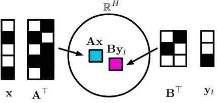
Model To leverage the relationships among the fine grained labels, we would like a model that can learn an embedding space for labels. Our model, based on WSABIE, learns to map both feature
vec-tors and labels to a low dimensional space RH (H is the embedding dimension size) such that each instance is close to its label(s) in this space; see Figure 2 for an illustration. Relationships be-tween labels are captured by their distances in the embedded space: co-occurring labels tend to be closer, whereas mutually exclusive labels are fur-ther apart.
Formally, we are interested in learning the map-ping functions:
f(x) :RD →RH
∀t∈ {1,2, . . . , T}, g(yt) :{0,1}T →RH
In this work, we parameterize them as linear func-tionsf(x,A) =Axandg(yt,B) =Byt, where
A∈RH×D andB∈RH×T are parameters. The score of a labelt(represented as a one-hot label vector yt) and a feature vectorxis the dot
A> B> yt
x
Ax Byt
RH
Figure 2: An illustration of the standard WSABIEmodel.
xis the feature vector extracted from a mention, andytis its label. Here, black cells indicate non-zero and white cells indicate zero values. The parameters are matricesAandB
which are used to map the feature vectorxand the label vec-torytinto an embedding space.
product between their embeddings:
s(x,yt;A,B) =f(x,A)·g(yt,B) =Ax·Byt For brevity, we denote this score bys(x,yt). Note that the total number of parameters is(D+T)×H, which is typically less than the number of pa-rameters in standard classification models that use regular conjunctions of input features with label classes (e.g., logistic regression) whenH < T. Learning Since we expect the training data to contain some extraneous labels, we use a ranking loss to encourage the model to place positive la-bels above negative lala-bels without competing with each other. LetYdenote the set of positive labels for a mention, and let Y¯ denote its complement. Intuitively, we try to rank labels inYhigher than labels inY¯. Specifically, we use the weighted ap-proximate pairwise (WARP) loss of Weston et al. (2011). For a mention{x,y}, the WARP loss is:
X
t∈Y X
¯ t∈Y¯
R(rank(x,yt)) max(1−s(x,yt) +s(x,y¯t),0)
where rank(x,yt) is the margin-infused rank of label t: rank(x,yt) = Pt¯∈Y¯I(1 + s(x,y¯t) >
[image:2.595.308.523.219.321.2]each mention can have multiple positive labels, we choose to optimize precision at k by setting
R(k) =Pki=1 1i. Favoring precision over recall in fine grained entity type classification makes sense because if we are not certain about a particular fine grained label for a mention, we should use its an-cestor label in the hierarchy.
In order to learn the parameters with this WARP loss, we use stochastic (sub)gradient descent.
Inference During inference, we consider the top-k predicted labels, where k is the maximum depth of the label hierarchy, and greedily remove labels that are not consistent with other labels (i.e., not on the same path of the tree). For example, if the (ordered) top-klabels areperson,artist, and location, we output only person and
artistas the predicted labels. We use a thresh-oldδ such thatyˆt= 1ifs(x,yt)> δ andyˆt = 0 otherwise.
Kernel extension We extend the WSABIE
model to include a weighting function between each feature and label, similar in spirit to We-ston et al. (2014). Recall that the WSABIE
scoring function is: s(x,yt) = Ax · Byt =
P
d(Adxd)>Bt, whereAdandBtdenote the col-umn vectors of A and B. We can weight each (feature, label) pair by a kernel function prior to computing the embedding:
s(x,yt) =
X
d
Kd,t(Adxd)>Bt,
where K ∈ RD×T is the kernel matrix. We use a N-nearest neighbor kernel2 and set K
d,t = 1 if Ad is one ofN-nearest neighbors of the label vector Bt, and Kd,t = 0 otherwise. In all our experiments, we setN = 200.
To incorporate the kernel weighting function, we only need to make minor modifications to the learning procedure. At every iteration, we first compute the similarity between each feature em-bedding and each label emem-bedding. For each label
t, we then set the kernel values for the N most similar features to 1, and the rest to 0 (updateK). We can then follow the learning algorithm for the standard WSABIE model described above. At
in-ference time, we fix K so this extension is only slightly slower than the standard model.
2We explored various kernels in preliminary experiments
and found that the nearest neighbor kernel performs the best.
The nearest-neighbor kernel introduces nonlin-earities to the embedding model. It implicitly plays the role of a label-dependent feature selector, learning which features can interact with which la-bels and turns off potentially noisy features that are not in the relevant label’s neighborhood.
3 Experiments
Setup and Baselines We evaluate our methods on two publicly available datasets that are man-ually annotated with gold labels for fine grained entity type classification: GFT (Google Fine
Types; Gillick et al., 2014) and FIGER(Ling and
Weld, 2012). On the GFT dataset, we compare
with state-of-the-art baselines from Gillick et al. (2014): flat logistic regression (FLAT), an
exten-sion of multiclass logistic regresexten-sion for multilabel classification problems; and multiple independent binary logistic regression (BINARY), one per label t∈ {1,2, . . . , T}. On the FIGERdataset, we
com-pare with a state-of-the-art baseline from Ling and Weld (2012).
We denote the standard embedding method by WSABIEand its extension by K-WSABIE. We fix
our embedding size toH = 50. We report micro-averaged precision, recall, and F1-score for each of the competing methods (this is calledLoose Mi-croby Ling and Weld). When development data is available, we use it to tune δ by optimizing F1-score.
Training data Because we have no manually annotated data, we create training data using the technique described in Gillick et al. (2014). A set of 133,000 news documents are automatically an-notated by a parser, a mention chunker, and an entity resolver that assigns Freebase types to en-tites, which we map to fine grained labels. This approach results in approximately 3 million train-ing examples which we use to train all the mod-els evaluated below. The only difference between models trained for different tasks is the mapping from Freebase types. See Gillick et al. (2014) for details.
Feature Description Example
Head The syntactic head of the mention phrase “Obama” Non-head Each non-head word in the mention phrase “Barack”, “H.” Cluster Word cluster id for the head word “59”
Characters Each character trigram in the mention head “:ob”, “oba”, “bam”, “ama”, “ma:” Shape The word shape of the words in the mention phrase “Aa A. Aa”
Role Dependency label on the mention head “subj”
Context Words before and after the mention phrase “B:who”, “A:first” Parent The head’s lexical parent in the dependency tree “picked”
[image:4.595.110.492.62.164.2]Topic The most likely topic label for the document “politics”
Table 1:List of features used in our experiments, similar to features in Gillick et al. (2014). Features are extracted from each mention. The example mention in context is... who Barack H. Obama first picked ....
GFTDev GFTTest FIGER
Total mentions 6,380 11,324 778
at Level 1 3,934 7,975 568
at Level 2 2,215 2,994 210
[image:4.595.83.282.215.269.2]at Level 3 251 335 –
Table 2:Mention counts in our datasets.
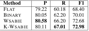
GFTevaluation There areT = 86fine grained
labels in the GFTdataset, as listed in Figure 1. The
four top-level labels are: person, location,
organization, andother; the remaining la-bels are subtypes of these lala-bels. The maximum depth of a label is 3. We split the dataset into a development set (for tuning hyperparameters) and test set (see Table 2).
The overall experimental results are shown in Table 3. Embedding methods performed well. Both WSABIE and K-WSABIE outperformed the
baselines by substantial margins in F1-score, though the advantage of the kernel version over the linear version is only marginally significant.
To visualize the learned embeddings, we project label embeddings down to two dimensions using PCA in Figure 3. Since there are only 4 top-level labels here, the fine grained labels are color-coded according to their top-level labels for readability. We can see that related labels are clustered to-gether, and the four major clusters correspond to to the top-level labels. We note that these first two components only capture 14% of the total variance of the full 50-dimensional space.
Method P R F1
FLAT 79.22 60.18 68.40
BINARY 80.05 62.20 70.01 WSABIE 80.58 66.20 72.68 K-WSABIE 80.11 67.01 72.98
Table 3:Precision (P), Recall (R), and F1-score on the GFT
test dataset for four competing models. The improvements for WSABIEand K-WSABIEover both baselines are
statisti-cally significant (p <0.01).
-0.4 -0.2 0.0 0.2 0.4 0.6 0.8
-0.6 -0.4 -0.2 0.0 0.2 0.4 0.6 PC1 P C2 organization company broadcastnews education government military music political_party sports_league sports_team stock_exchangetransit location celestial city country geography body_of_water island mountain park structure airport hospital hotel restaurant
sports_facilitytransittheater bridge railway road other art broadcast film music stage writing award body_part currency event accident election holiday natural_disaster sports_event violent_conflict food health malady treatment heritage internet language programming_language legal living_thinganimal product car computer mobile_phone software scientific sports_and_leisure supernatural person artist actor author director music athlete business coach doctor education teacher legal military political_figure religious_leader title organization location other person
Figure 3: Two-dimensional projections of label embed-dings for GFTdataset. See text for details.
FIGER evaluation Our second evaluation
dataset is FIGER from Ling and Weld (2012). In
this dataset, there areT = 112labels organized in a two-level hierarchy; however, only 102 appear in our training data (see Figure 1, taken from their paper, for the complete set of labels). The training labels include 37 top-level labels (e.g., person, location, product, art, etc.) and 75 second-level labels (e.g., actor,
city,engine, etc.) The FIGERdataset is much
smaller than the GFTdataset (see Table 2).
Our experimental results are shown in Ta-ble 4. Again, K-WSABIE performed the best,
followed by the standard WSABIE model. Both
of these methods significantly outperformed Ling and Weld’s best result.
Method P R F1
Ling and Weld (2012) – – 69.30 WSABIE 81.85 63.75 71.68
[image:4.595.105.257.661.714.2]K-WSABIE 82.23 64.55 72.35
Table 4: Precision (P), Recall (R), and F1-score on the FIGERdataset for three competing models. We took the F1 score from Ling and Weld’s best result (no precision and re-call numbers were reported). The improvements for WSABIE
and K-WSABIEover the baseline are statistically significant
Feature learning We investigate whether hav-ing a large fine grained label space is helpful in learning a good representation for feature vec-tors(recall that WSABIElearns representations for
both feature vectors and labels). We focus on the task of coarse type classification, where we want to classify a mention into one of the four top-level GFTlabels. We fix the training mentions and learn
WSABIE embeddings for feature vectors and
la-bels by (1) training only on coarse lala-bels and (2) training on all labels; we evaluate the models only on coarse labels. Training with all labels gives an improvement of about 2 points (F1 score) over training with just coarse labels, as shown in Ta-ble 5. This suggests that including additional sub-type labels can help us learn better feature embed-dings, even if we are not explicitly interested in the deeper labels.
Training labels P R F1
Coarse labels only 82.41 77.87 80.07 All labels 85.18 79.28 82.12
Table 5: Comparison of two WSABIEmodels on coarse type classification for GFT. The first model only used coarse
top-level labels, while the second model was trained on all 86 labels.
4 Discussion
Design of fine grained label hierarchy Results at different levels of the hierarchies in Table 6 show that it is more difficult to discriminate among deeper labels. However, it appears that the depth-2 FIGERtypes are easier to discriminate than the
depth-2 (and depth-3) GFTlabels. This may
sim-ply be an artifact of the very small FIGERdataset,
but it suggests it may be worthwhile to flatten the
othersubtree ini GFTsince many of its subtypes
do not obviously share any information.
GFT P R F1
LEVEL1 85.22 80.55 82.82
LEVEL2 56.02 37.14 44.67
LEVEL3 65.12 7.89 14.07
FIGER P R F1
LEVEL1 82.82 70.42 76.12
LEVEL2 68.28 47.14 55.77
Table 6: WSABIEmodel’s Precision (P), Recall (R), and F1-score at each level of the label hierarchies for GFT(top) and FIGER(bottom).
5 Conclusion
We introduced embedding methods for fine grained entity type classifications that outperforms state-of-the-art methods on benchmark entity-classification datasets. We showed that these
methods learned reasonable embeddings for fine-type labels which allowed information sharing across related labels.
Acknowledgements
We thank Andrew McCallum for helpful discus-sions and anonymous reviewers for feedback on an earlier draft of this paper.
References
Andrew Carlson, Justin Betteridge, Richard C. Wang, Estevam R. Hruschka Jr., and Tom M. Mitchell. 2010. Coupled semi-supervised learning for infor-mation extraction. InProc. of WSDM.
R. Collobert, J. Weston, L. Bottou, M. Karlen, K. Kavukcuoglu, and P. Kuksa. 2011. Natural lan-guage processing (almost) from scratch. Journal of Machine Learning Research, 12:2493–2537. George Doddington, Alexis Mitchell, Mark Przybocki,
Lance Ramshaw, Stephanie Strassel, and Ralph Weischedel. 2004. The automatic content extrac-tion (ACE) program tasks, data, and evaluaextrac-tion. In Proc. of LREC.
Kuzman Ganchev and Mark Dredze. 2008. Small sta-tistical models by random feature mixing. In Pro-ceedings of the ACL08 HLT Workshop on Mobile Language Processing, pages 19–20.
Dan Gillick, Nevena Lazic, Kuzman Ganchev, Jesse Kirchner, and David Huynh. 2014. Context-dependent fine-grained entity type tagging. In arXiv.
Lynette Hirschman and Nancy Chinchor. 1997. MUC-7 named entity task definition. InProc. of MUC-7. Thomas Lin, Mausam, and Oren Etzioni. 2012. No
noun phrase left behind: Detecting and typing un-linkable entities. InProc. of EMNLP-CoNLL. Xiao Ling and Daniel S. Weld. 2012. Fine-grained
entity recognition. InProc. of AAAI.
Yanjun Qi, Sujatha Das G, Ronan Collobert, and Jason Weston. 2014. Deep learning for character-based information extraction. InProc. of ECIR.
Marta Recasens, Marie-Catherine de Marneffe, and Christopher Potts. 2013. The life and death of dis-course entities: Identifying singleton mentions. In Proc. of NAACL.
Erik F. Tjong Kim Sang and Fien De Meulder. 2003. Introduction to the conll-2003 shared task: language-independent named entity recognition. In Proc. of HLT-NAACL.
Joseph Turian, Lev Ratinov, and Yoshua Bengio. 2010. Word representations: A simple and general method for semi-supervised learning. InProc. of ACL. Jason Weston, Samy Bengio, and Nicolas Usunier.
2011. Wsabie: Scaling up to large vocabulary im-age annotation. InProc. of IJCAI.
Jason Weston, Ron Weiss, and Hector Yee. 2014. Affinity weighted embedding. InProc. of ICML. Limin Yao, Sebastian Riedel, and Andrew McCallum.
2010. Collective cross-document relation extraction without labelled data. InProc. of EMNLP.