© 2019, IRJET | Impact Factor value: 7.211 | ISO 9001:2008 Certified Journal
| Page 5932
GDP Forecast for India using Mixed Data Sampling technique
Abanish S Vijay
1, Asok Kumar N
21
Department of Mechanical Engineering, College of Engineering Trivandrum
2
Assistant Professor, Department of Mechanical Engineering, College of Engineering Trivandrum
---***---Abstract -
Gross Domestic Product is the monetary measureof all the goods and service produced in a country in a given time period. GDP calculation is important as it helps in assessing the economic health of a country. By forecasting the GDP, policy makers of a country can make decisions so as to ensure that economic development progresses unhindered and to reduce the chances of economic recession. This project work attempts to develop an efficient method to forecast the GDP of India using Mixed Data Sampling Technique. The GDP of India is affected by various macroeconomic indicators which vary in quarterly, monthly, weekly or daily frequencies. A preliminary study was conducted in order to identify the macroeconomic indicators affecting the GDP of India. After identifying the indicators, the Dynamic Factor Modelling method was first used to identify the relevant predictors from large amounts of macroeconomic and financial data affecting Indian Economy. After identifying 22 relevant predictors, the Mixed Data Sampling Technique was implemented in order to obtain the GDP Forecast. . Both the forecasts were compared by calculating the Root Mean Square Forecast Error in order to ascertain the accuracy of the MIDAS technique. Then the Diebold Mariano test was conducted in order to identify whether there was a significant difference between the GDP Forecasts.
Key Words: Dynamic Factor Modelling, Mixed Data Sampling Technique, Root Mean Square Forecast Error, Linear Regression, Diebold Mariano Test.
1. INTRODUCTION
Gross Domestic Product(GDP) Forecast of India is done by several government entities such as Central Statistical Office, Niti ayog, Reserve Bank of India, International agencies such as World Bank, International Monetary Fund and Asian Development Bank and several private entities such as Fitch, Moody’s, standard and poor’s etc. The GDP forecast given by these entities usually have significant variation between each other. In order to avoid this situation and to get an accurate forecast, all the macroeconomic indicators affecting the GDP has to be used during the forecasting procedure.
After collecting all the macroeconomic indicators affecting the GDP of a country, the relevant predictors which have a bearing on the actual GDP has to be identified. If all the collected data is used for the forecast without an initial filtering, more errors can creep in to the forecast. In order to prevent this, a novel method called Dynamic Factor
Modelling (DFM) is used. After conducting DFM on the data collected, the relevant predictors which affect GDP can be identified.
The predictors which are obtained through DFM varies on a quarterly, monthly, weekly or daily basis. This variation in predictor frequency makes it difficult to obtain the GDP Forecast. In the currently followed traditional method of forecast, the predictors having higher frequency of occurrence are averaged to lower frequency and forecast is carried out at the lower frequency. For example, monthly economic indicators are averaged to obtain quarterly data and it is used for forecast along with quarterly economic indicators. This method of forecast has some draw backs as lot of valuable data are lost during averaging and frequency conversion. To counter this problem, Mixed Data Sampling (MIDAS) Technique can be used [1](Ghysels et al., 2004). By using MIDAS method, the need for averaging higher frequency indicators is eliminated and the forecast can be carried out including all the observations.
Literature survey revealed that, Dynamic Factor Modelling and Mixed Data Sampling Technique has not been implemented in the forecast of India’s GDP. Hence, this study was conducted with the objective of determining the relevant predictors affecting India’s GDP from a large number of macroeconomic indicators and to identify the GDP of India using MIDAS technique. The results of this study should be an appropriate basis to lay down a better GDP forecast methodology for India. The result obtained through the method will be compared with the result obtained through traditional methods in order to identify the advantage of the MIDAS technique. A hypothesis testing method is used to assess the superiority of the MIDAS method over the traditional regression method.
1.1 Importance of forecasting GDP
Gross domestic product (GDP) is arguably a key macroeconomic indicator, indicating where the economy is in the cycle and feeding very prominently into economic policymaking. In particular, appropriate policy formulation and implementation require not only to examine GDP’s historical development but also to predict its current and future path, to enable prompt responses to changes in economic conditions. Accurate and timely information on GDP is thus crucial.[2](Sathoshi Urasawa., 2014).
© 2019, IRJET | Impact Factor value: 7.211 | ISO 9001:2008 Certified Journal
| Page 5933
of business in general and of economics in particular. Theissues of GDP has become the most concerned amongst macro economy variables and data on GDP is regarded as the important index for assessing the national economic development and for judging the operating status of macro economy as a whole [3](Ning et al. 2010).
1.2 Dynamic Factor Modelling
The dynamic factor model (DFM) is applied to extract dynamic factors as predictors from large amounts of macroeconomic and financial data. The DFM has two advantages. First, the idiosyncratic parts of the DFM are allowed to be auto correlated and have heteroscedasticity in both the time and the cross-section dimension, which is especially suitable for the financial time series. Second, the DFM allows factor loadings to change with time, which can effectively solve the issue of instability that may exist in the data due to the nonstationary or the existence of structural breaks of the time series [4](Yu Jiang., 2017). The Dynamic Factor Model is given as follows.
(1.1) (1.2)
Where is a N× k lag polynomial matrix of degree p, is a k×1 vector containing k dynamic factors at time t, is a N × 1 vector of error terms, is a k × k lag polynomial matrix of degree q, is a K × 1 vector of error terms [5] (Zhiyuan Pan et al., 2018).
1.3 Mixed Data Sampling Technique
A typical time series regression model involves data sampled at the same frequency. The idea to construct regression models that combine data with different sampling frequencies is relatively unexplored. We discuss various ways to construct such regressions. We call the regression framework a Mi(xed) Da(ta) S(ampling) regression (henceforth MIDAS regression). At a general level, the interest in MIDAS regressions addresses a situation often encountered in practice where the relevant information is high frequency data, whereas the variable of interest is sampled at a lower frequency. One example pertains to models of stock market volatility. The low frequency variable is for instance the quadratic variation or other volatility process over some long future horizon corresponding to the time to maturity of an option, whereas the high frequency data set is past market information potentially at the tick-by-tick level. MIDAS regressions can also result from limitations to data availability. For example, some macroeconomic data are sampled monthly, like price series and monetary aggregates, whereas other series are sampled quarterly or annually, typically real activity series like GDP and its components. Take for instance the
relationship between inflation and growth. Instead of aggregating the inflation series to a quarterly sampling frequency to match GDP data, one can run a MIDAS regression combining monthly and quarterly data [6]( Stock et al., 2004). An h step ahead GDP forecast using MIDAS Technique is given by
(1.3)
Where is the order of lags of , is the order of lags of monthly predictors, ,α,β are the coefficients to be estimated and is the error term
2. METHODOLOGY
A preliminary study was conducted to identify the macroeconomic indicators affecting the GDP of India. After identifying the macroeconomic indicators, dynamic factor modelling is carried out to identify the relevant predictors which play a major role in determining the GDP forecast of India. The identified relevant predictors are used to forecast the GDP by using the MIDAS technique. A quarter ahead forecast is obtained and in order to ascertain the accuracy of the method, a forecast using traditional regression method is carried out [7] (Andreou .,2013). The forecast obtained using MIDAS method and traditional forecast method is compared together to ascertain the accuracy of the method. Root Mean Square Forecast Error (RMSFE) of the two forecast values are calculated to compare the accuracy of the method. After finding the RMSFE, Diebold-Mariano test is carried out to ascertain the significance of variation between the two forecasts.
2.1 Preliminary study to identify the Maroeconomic
indicators affecting the GDP of India
© 2019, IRJET | Impact Factor value: 7.211 | ISO 9001:2008 Certified Journal
| Page 5934
2.2 Data Collection
The GDP data for the period from 1996-2018 was collected from the Data Base of Indian Economy maintained by the Reserve Bank of India. Data on Consumer Price Index and Wholesale Price Index for the corresponding periods were collected from the Central Statistical Office (CSO) database. Data varying over weekly frequencies such as foreign currency assets, Gold reserves, Currency in circulation, Foreign Exchange Assets and Reserve Money was collected from the Data Base on Indian Economy. Daily varying data such as Collateralized Borrowing and Lending Obligation (CBLO) data and Market Repo data were also collected from the Data Base on Indian Economy. Each of the above said data variables had several components which constituted them and they were individually collected for the data analysis. A total of 38 macroeconomic indicators for the captioned period was collected from various sources.
2.3 Dynamic Factor Modelling
All the collected macroeconomic indicators cannot be used together for the GDP forecast. The relevant indicators which affect GDP are to be identified in order to get an accurate GDP Forecast. Dynamic Factor Analysis technique was used for identifying the relevant predictors. The data we have collected is a time series data and Dynamic Factor Analysis is most suited for analysing time series data. The mathematical model for Dynamic Factor Analysis was discussed in the literature review section [8]( Timmermann.,2006)
.
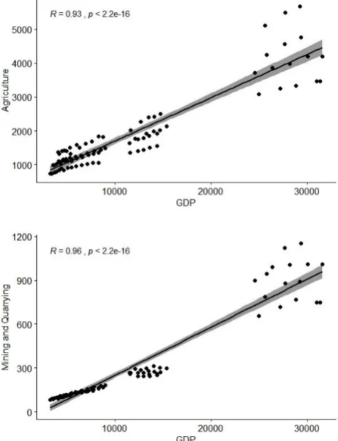
DFA relies on the fit of the data variables with the common trend. A Dynamic Factor Model can be seen as a regression model with the underlying assumptions namely, Normality, Independence and Homogeneity of the data points. Dynamic Factor Analysis involves transforming the data points in to a common time line and analysing the correlation coefficient for identifying homogeneity. If the analysis indicates a combination of non normality, heterogeneity and serial correlation of residuals the macroeconomic indicator is not a relevant predictor and can be rejected [9] (A.F. Zuur.,2003). All the 38 macroeconomic indicators were individually analysed using R software and by analysing the correlation coefficient, the relevant indicators which affect GDP forecast are identified. The result of the Dynamic Factor Analysis study conducted on the 8 quarterly components of GDP is given in figure 2.1 [image:3.595.311.557.102.423.2]It can be seen that even if the correlation coefficient is high, the plot might not be homogeneous, this will lead to rejection of the macroeconomic indicator as a relevant predictor. The plot should be homogeneous and converging in order for the indicators to be accepted as a relevant predictor. So for identifying the relevant predictor, the correlation coefficient and the convergence diagram is to be analysed together.
Fig -2.1: Dynamic Factor Analysis on components of GDP
It can be observed that the data indicators with the lowest correlation coefficient and the least linearity in their time series distribution are rejected. In this case, Agriculture, Mining and Quarrying and Transportation data are rejected because of their non-linear nature in comparison with the other data points. In a similar manner all the other macroeconomic indicators are analysed and the relevant predictors are identified. The result of the Dynamic Factor Analysis on Monthly Consumer Price Index data is given in figure 2.2.
© 2019, IRJET | Impact Factor value: 7.211 | ISO 9001:2008 Certified Journal
| Page 5935
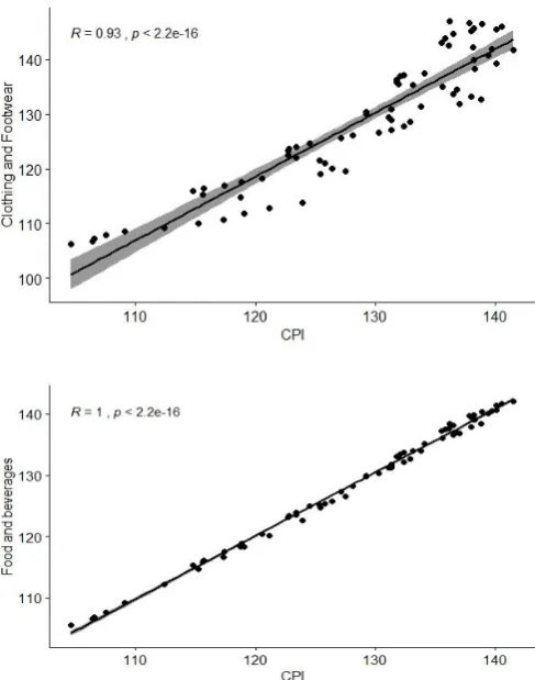
Fig-2.2:Dynamic Factor Analysis on Consumer Price IndexIn a similar manner Dynamic Factor Analysis was conducted on all the 38 macroeconomic indicators. The relevant predictors identified through this analysis are given below in Table 2.1
Table -2.1: Macroeconomic indicators selected for GDP Forecast
Sl.No Frequency Macroeconomic Indicators selected after DFA
1 Quarterly Manufacturing, Electricity, Construction, Finance, Public administration and Defence.
2 Monthly Clothing and Footwear(CPI),
Food and beverages(CPI), Housing(CPI),
Miscellaneous(CPI), Pan&Tobacco(CPI), Food Articles(WPI), Manufactured Products(WPI), Mineral Oils(WPI), Minerals(WPI), Non Food articles(WPI)
3 Weekly Foreign currency assets, Gold
reserves, Currency in
circulation, Foreign Exchange Assets, Reserve Money.
4 Daily Collateralized Borrowing and
Lending Obligation, Market Repo
2.3 Implementing Mixed Data Sampling
The collected Macroeconomic indicators are used for forecasting the GDP using MIDAS technique. The analysis is carried out with Econometric views software. The selected macroeconomic indicators are imported individually in to the user interface of the software and GDP Forecast using MIDAS technique is carried out. We give lags of one quarter in order to obtain the forecast. However while importing the data, they have to be separately specified based on the frequency in which they are distributed.
2.4 GDP Forecast using Averaging and Linear
Regression
In order to know the accuracy of MIDAS technique over traditional methods, GDP forecast was done after averaging the macroeconomic indicators to a common frequency and conducting linear regression.The data indicators distributed over monthly, weekly and daily frequencies were averaged to quarterly frequency and was then imported in to the EViews software. After this, linear regression was conducted in order to forecast the GDP. One quarter ahead GDP forecast was obtained through linear regression by giving a lag of one period[10](
Stock
et al.,2006)The results obtained through both of the methods are compared with each other.3 Results and Discussions
The results of the work are described below in the different sections. The results of GDP Forecast obtained through MIDAS method and linear regression method are described in detail. The results of comparison between the two forecasts are also given in subsequent sections.
3.1 GDP Forecast through MIDAS Technique
The data until the third quarter of 2018 was imported in to the EViews software. After processing the data in EViews, GDP growth rate for the period from first quarter of 2016 to the last quarter of 2018 was generated. Thus one quarter ahead forecast was obtained. The GDP forecasted through MIDAS technique is given in Table 3.1.
Table-3.1: GDP Forecast using MIDAS Technique
Quarter GDP growth rate
2016 Q1 2.987471
2016 Q2 2.019939
2016 Q3 -0.248808
2016 Q4 1.903544
2017 Q1 2.162267
2017 Q2 1.588072
2017 Q3 0.294494
2017 Q4 2.368801
© 2019, IRJET | Impact Factor value: 7.211 | ISO 9001:2008 Certified Journal
| Page 5936
2018 Q2 1.970872
2018 Q3 -0.71795
2018 Q4 2.800339
3.2 GDP Forecast through Linear Regression
The macroeconomic indicators which vary over daily frequencies were averaged over a period of 90 days, and those indicators which vary over weekly frequencies were averaged over a period of 16 weeks and those which varied in a monthly basis was averaged over a period of three months. This data was then fed in to the EViews software and the GDP Forecast from the first quarter of 2016 to the last quarter of 2018 was obtained. The generated values are given below in Table 3.2.
Table-3.2: GDP forecast using Linear Regression
Quarter GDP growth rate
2016 Q1 2.650684
2016 Q2 2.372294
2016 Q3 2.224945
2016 Q4 2.027771
2017 Q1 2.671941
2017 Q2 2.592534
2017 Q3 2.128170
2017 Q4 2.522358
2018 Q1 2.625201
2018 Q2 2.463240
2018 Q3 -0.218135
2018 Q4 2.455532
3.3 Root Mean Square Forecast Error
Root Mean Square Forecast Error helps in assessing the accuracy of the forecast. The actual value of GDP growth is calculated from the previously collected GDP data and the Root Mean Square Forecast Error (RMSFE) is calculated based on the equation given below.
RMSFE
=
(3.1)Where is the Forecasted GDP, is the actual GDP and ‘n’ is the number of observations in the GDP Forecast. The value of actual GDP and RMSFE for the GDP forecasted through two methods are given below in table 4.3
Table-3.3: Root Mean Square Forecast Error of the two forecasts.
Sl. No
Actual GDP Growth (AGi)
MIDAS Forecast (MGi)
Square of (AGi-MGi)
Regression Forecast (RGi)
Square of (AGi-RGi)
1 3.032 2.988 0.00203 2.6506 0.145816
2 2.040 2.0199 0.00042 2.3722 0.110102
3 -0.248 -0.249 9.5648E-08 2.2249 6.117925
4 1.922 1.904 0.00033244 2.0277 0.011235
5 2.186 2.162 0.00055444 2.6719 0.236318
6 1.601 1.588 0.0001607 2.5925 0.983638
7 0.295 0.294 1.8841E-07 2.12817 3.360776
8 2.397 2.368 0.0007997 2.522 0.015695
9 3.080 3.033 0.00216049 2.6252 0.206873
10 1.990 1.970 0.0003822 2.4632 0.223557
11 -0.715 -0.717 6.6108E-06 -0.218 0.24739
12 2.913 2.800 0.01265503 2.4555 0.209125
RMSFE 0.040317 0.9945
From the Root Mean Square values of the two forecasts, it can be observed that MIDAS forecast has less error as compared to Regression forecast. However in order to ascertain whether there is any significant difference in the forecasts, a Hypothesis Test can be carried out.
3.4 Diebold Mariano Test
In Diebold Mariano Test, we have to test the null hypothesis H0: E(dt) = 0 ∀t versus the alternative hypothesis H1 : E(dt) ≠ 0. The null hypothesis is that the two forecasts have the same accuracy and the alternative hypothesis is that the two forecasts have different levels of accuracy. Suppose that the forecasts are h>1 step ahead. In order to test the null hypothesis that the two forecasts have the same accuracy, Diebold Mariano test utilizes the following statistic
DM
=
(3.2)© 2019, IRJET | Impact Factor value: 7.211 | ISO 9001:2008 Certified Journal
| Page 5937
must be split such that 0.025 is in the upper tail and another0.025 in the lower. The z-value that corresponds to -0.025 is -1.96, which is the lower critical z-value. The upper value corresponds to 0.975 or (1-.025), which gives a Z-value of 1.96. The null hypothesis of no difference will be rejected if the computed DM statistic falls outside the range of -1.96 to 1.96. The DM test was carried out using R software after inputting the squared error values in the actual GDP and the forecasted GDP values. MultDM package in R was used for conducting the DM test. After conducting the test a P value of less than 2.2e-16 was obtained, this falls outside the range of -1.96 to 1.96. Based on this we are able to reject the null hypothesis that both of the forecasts have equal accuracy.
Now based on the results obtained from the calculation of Root Mean Square Forecast Error and Diebold Mariano test, we can conclude that GDP forecast using MIDAS technique is superior to that of traditional methods of forecasting.
4 CONCLUSIONS
GDP forecast is important for policy makers to make necessary decisions to ensure that the economic growth keeps moving forward. It enables policy makers to make necessary decisions such as fixing market repo rate, increasing or decreasing the interest rate etc so as to improve the economy of the country. It also enables policy makers to keep the price inflation in check so as to prevent uncontrollable rising of prices. If GDP forecast is standardized across all government agencies it can lead to long lasting advantages in terms of economic prosperity and growth.
Results of Dynamic Factor Analysis enabled us to identify the relevant predictors affecting GDP forecast from the large number of economic indicators which affects the economy of India. The relevant predictors seems to be an accurate indicator of the GDP growth rate in India. After finding the relevant predictors, the next problem was in calculating the GDP forecast with the relevant predictors which varied over different frequencies. MIDAS technique was helpful in overcoming this problem. After calculating the GDP using the MIDAS technique, the GDP was forecasted using linear regression method in order to ascertain the accuracy of the MIDAS method. In the linear regression method, the GDP was forecasted after averaging all the relevant predictors to a common data frequency. After both the forecasts were obtained, we tested the accuracy of the method using Root Mean Square Forecast Error and DM test method.
From the result of Root Mean Square Forecast Error, it was evident that GDP forecast using MIDAS method has less error as compared to the linear regression method. Further in order to ascertain the statistical significance of the variation in forecast accuracy, DM test was conducted. Based on the lower P Value obtained as a result of the DM test it can be concluded that the accuracy of both the forecasts are not the
same. The null hypothesis that both the accuracies were similar was rejected. This itself is an indicator that GDP forecast using MIDAS method is better than GDP forecast using traditional techniques. It can also be seen that the GDP forecast values obtained through MIDAS technique are closer to the actual GDP values than the traditional regression methods.
There is further scope for study in this topic as we have only used the Almon technique of MIDAS forecast. There are still other technique such as step MIDAS Forecast, Beta MIDAS forecast etc which can lead to different values of the forecast. These techniques can be used and the results can be compared to arrive at a more accurate forecast. It may also be noted that GDP is affected by a large number of variables, so further research can be conducted by incorporating more economic indicators in order to improve the accuracy of the forecast. A standardized method for GDP forecast in India can be developed through further research in the topic. This will be beneficial for the policy makers and to the nation in general.
REFERENCES
[1] Ghysels, E., Santa-Clara, P., Valkanov, R., 2004. The MIDAS Touch: Mixed Data Sampling Regressions. Mimeo. Chapel Hill
[2] Satoshi Urasawa (2014) Japan’s deflation: the role of wage costs, Applied Economics Letters, 21:11, 742-746 [3] Ning, W., Kuan-jiang, B. and Zhi-fa, Y. (2010), Analysis and forecast of Shaanxi GDP based on the ARIMA Model, Asian Agricultural Research, Vol. 2 No. 1, pp. 34-41. [4] Yu Jiang, Yongji Guo, Yihao Zhang. (2017). Forecasting
China's GDP growth using dynamic factors and mixed-frequency data, Economic Modelling, JEL C53 E17. [5] Zhiyuan Pan, Qing Wang, Yudong Wanga, Li Yang.
(2018). Forecasting U.S. real GDP using oil prices: A time-varying parameter MIDAS model, Energy Economic, Eneeco 3978.
[6] Stock, J.H., Watson, M.W. (2004). Combination forecasts of output growth in a seven country data set, Journal of Economic Forecast, 23, 405–430.
[7] Andreou, E., Ghysels, E., Kourtellos, A. (2013). Should macroeconomic forecasters use daily financial data and how, Journal of Business Economics, 31 (2), 240–251. [8] Timmermann, A. (2006). Forecast combinations,
Handbook of Economic Forecasting, vol. 1, pp. 136–196. [9] A.F. Zuur., I.D. Tuck., N. Bailey. (2003). Dynamic factor analysis to estimate common trends in fisheries time series, NRC Research Press Web site.
[10]Stock, J.H., Watson, M.W, 2006. Forecasting with many predictors. Handbook of Economic Forecasting, pp. 515– 554.