Synchronization controller for a 3 RRR parallel manipulator

warwick.ac.uk/lib-publications

Original citation:

Nguyen, Khoa Dang, Ha, Cheolkeun, Dinh, Quang Truong and Marco,

James (2018) Synchronization controller for a 3-RRR parallel manipulator. International

Journal of Precision Engineering and Manufacturing, 19 (3). pp.

339-347. doi:

10.1007/s12541-018-0041-z

Permanent WRAP URL:

http://wrap.warwick.ac.uk/101029

Copyright and reuse:

The Warwick Research Archive Portal (WRAP) makes this work by researchers of the

University of Warwick available open access under the following conditions. Copyright ©

and all moral rights to the version of the paper presented here belong to the individual

author(s) and/or other copyright owners. To the extent reasonable and practicable the

material made available in WRAP has been checked for eligibility before being made

available.

Copies of full items can be used for personal research or study, educational, or not-for profit

purposes without prior permission or charge. Provided that the authors, title and full

bibliographic details are credited, a hyperlink and/or URL is given for the original metadata

page and the content is not changed in any way.

Publisher’s statement:

“The final publication is available at Springer via

http://dx.doi.org/10.1007/s12541-018-0041-z

”

A note on versions:

The version presented here may differ from the published version or, version of record, if

you wish to cite this item you are advised to consult the publisher’s version. Please see the

‘permanent WRAP url’ above for details on accessing the published version and note that

access may require a subscription.

DOI: XXX-XXX-XXXX

NOMENCLATURE

t

K= torque factor constant (Nm/A)

b

K = back EMF constant (V/rad/s)

b= damping ratio(N.m.s)

J=moment inertia (kgm2₎

a

R=armature resistance()

a

L =armature inductance (H)

a

i =armature current (A) =angle of the rotor (rad)

a

V =input voltage (V)

RRR = revolute-revolute-revolute joint PRR = prismatic-revolute-revolute joint

1. Introduction

In industrial applications, robots can be mainly classified into two categories, serial and parallel. While serial robots use an open-loop manipulator with one link connecting to the ground and others being free in the workspace, parallel robots use closed-loop mechanism with all links connecting to a fixed base and a moving platform which is controlled by component actuators. A parallel

robot offers higher accuracy, rigidity and lower inertia1 _{than a serial} robot. Therefore, parallel robots have attracted significant interests from both researchers and designers in many years. Especially, 3-RRR-type parallel robot is realized as one of the best solutions for various applications such as laser cutters, 3D printers, ships and flights’ simulators.

Performance of a 3-RRR parallel robot depends on its chairs which are activated independently by actuators. Different types of actuators have been used including Pneumatic Artificial Muscles (PAMs),2 _{RC servo motors,}3,4 _{DC motors}5,6,7 _{and AC servo motors.}8 Among them, DC motors have been mostly used due to its advanced characteristics as low cost and easy for monitoring by the support of encoder.

For any tracking task using the traditional approach, the component actuators are controlled separately to follow their own references which are derived from the desired trajectory of the end-effector. Hence, two critical issues need to be addressed. First, it is necessary to have an accurate inverse kinematic model to derive properly the actuators’ trajectories. Many studies have been presented the kinematic model and determined singularity of a parallel mechanism.9-11 _{The inverse kinematics}12-15 _{was analysed an} in-depth for the 3-RRR parallel robot. Second, a controller is needed for each actuator to achieve its given task. Several control

Synchronization controller for a 3-RRR parallel

manipulator

Khoa Dang Nguyen

1

_{, Cheokeun Ha}

1#

_{, Truong Quang Dinh}

2

_,

_and

_{James Marco}

2

1 School of Mechanical and Automotive Engineering, University of Ulsan, Namgu, Mugeodong, Ulsan 680-749, Korea 2 Warwick Manufacturing Group (WMG), University of Warwick, Coventry CV47AL, UK # Corresponding Author / E-mail: [email protected], TEL: +82-52-259-2550, FAX: +82-52-259-1682

KEYWORDS: Synchronization, Slide mode, Neural network, Stability, 3-RRR parallel robot

A 3-RRR parallel manipulator has been well-known as a closed-loop kinematic chain mechanism in which the end-effector generally a moving platform is connected to the base by several independent actuators. Performance of the robot is decided by performances of the component actuators which are independently driven by tracking controllers without acknowledging information from each other. The platform performance is degraded if any actuator could not be driven well. Therefore, this paper aims to develop an advanced synchronization (SYNC) controller for position tracking of a 3-RRR parallel robot using three DC motor-driven actuators. The proposed control scheme consists of three sliding mode controllers (SMC) to drive the actuators and a supervisory controller named PID-neural network controller (PIDNNC) to compensate the synchronization errors due to system nonlinearities, uncertainties and external disturbances. A Lyapunov stability condition is added to the PIDNNC training mechanism to ensure the robust tracking performance of the manipulator. Numerical simulations have been performed under different working conditions to demonstrate the effectiveness of the suggested control approach.

Manuscript received: August XX, 201X / Revised: August XX, 201X / Accepted: August XX, 201X

solutions of planar parallel robots have been known as the PID controller,16 _{PID-like fuzzy logic controller,}17 _{semi-closed-loop} controller,5 _{simple fuzzy controller,}2 _{sliding mode controller.}18 Another trend is to design a control method based on dynamic model of 3-RRR parallel robots such as intelligent active force and fuzzy controller,19 _{the combination between PID and active force} controller(AFC),20,21 _{nonlinear computed torque controller(CTC),}22 nonlinear PD-CTC23 _{and nonlinear PD.}24

Although the developed control systems showed some interesting results, their applicability is limited due to following reasons. First due to the system nonlinearities and uncertainties, it is difficult to develop an accurate inverse kinematic model to compute references for the component actuators. Second, each actuator is independently controlled without any communication with others. Subsequently, any tracking error due to the actuator trajectory definition or the controller could lead to a significant tracking error of the end-effector. The final robot performance is therefore totally deteriorated.

To overcome the shortcomings of the traditional control approaches for parallel robots, synchronization (or SYNC) control is known as one of the most feasible solutions which have been drawn a lots of attention from researchers in recent years. In a SYNC control system, a main controller is designed to keep tracking trajectory for each actuator and the SYNC is developed to compensate the errors between the actuators. DuyKhoa et al.2 developed a synchronization controller using adaptive neuron fuzzy inference system (ANFIS) for a 3-RRR planar parallel robot. Yuxin et al.25,26_{presented a combination between PI synchronous control} and PD feedback control for a parallel manipulator. Luren27 developed a synchronization controller for a 3-DOF planar robot by using the convex combination method. JungHwan et al.28 _{used PD} synchronization controller to compensate the tracking errors in dual parallel motion stages. In another study, the trajectory tracking control of a pneumatic X-Y table29 _{was synchronously driven by a} neural network based PID control scheme.

Although the efficiency of using the control approaches proposed in these studies was well presented by both the simulation and real experiments, the stability of these SYNC algorithms has not been stated. To develop a robust SYNC control for a 3-PRR parallel robot, Luren et al.30-32 _{presented an adaptive} synchronization control based on the dynamic model and forward kinematics. Su et al.33 _{also used dynamic model to design an} nonlinear PD synchronized control. Nevertheless, in this case the robot needs to be equipped with a proper sensor to detect the moving platform to derive the SYNC error. Consequently, the system becomes complex and expensive solution which limits its applicability. As another solution, the master-slave method34 _has applied for CNC machine tools with dual driving systems. However, this method is not suitable for parallel robot which includes self-sufficient components. In these studies, the Lyapunov stability constraints were introduced based on dynamic model of the robot to prove the robustness of the controllers. Therefore, the stability is difficult to establish for the difference robots.

In this paper, an advanced SYNC control approach is designed

for tracking control of a typical 3-RRR parallel robot. The robot contains a moving platform which is operated by three DC motor-driven actuators. First, based on the inverse kinematic model, a sliding mode controller (SMC) is designed to keep the each actuator to track its desired trajectory. Second, a supervisory controller named PID-based neural network controller (PIDNNC) is robustly constructed using Lyapunov stability condition to compensate the SYNC errors between the actuators due to the system nonlinearities, uncertainties and external disturbances. The SYNC errors therefore can converge simultaneously to zero to ensure the robust tracking performance of moving platform.

The remainder of this paper is organized as follows: Section 2 is the problem definition and mathematical model of the 3-RRR parallel robot while the design of the proposed control scheme is introduced in Section 3. Numerical simulations are then performed in Section 4 to verify the control effectiveness. Finally, some concluding remarks are given in Section 5.

2. Problem description and system modeling

2.1 3-RRR parallel robot

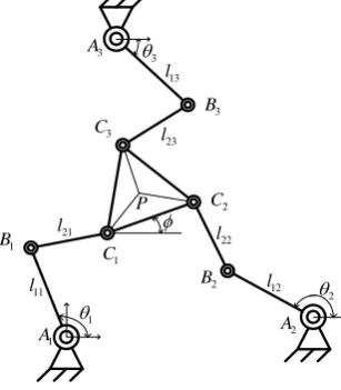
Configuration of the studied 3-RRR parallel robot is shown in Fig. 1. Herein, the robot contains a moving platform which is connected to a fixed base through three RRR serial chains and three rotating joints. Each chain includes two links with revolute joints and is driven by an active rotary actuator, such as electric servo motor.

The position and orientation of moving platform are in turn represented by P(x,y),



. For chain ith _{(i=1, 2, 3), let's define A}

i ,Bi ,Ci are the joints between the actuator-link1, link1-link2 and link2-moving platform, respectively; l1i , l2iare lengths of the link1 and link2, respectively;

  

₁, ,_{2 3} are the angular position of the three actuators.

1 

3 



11 l

21 l

12 l 22 l 23 l

13 l

2 

1

A A2

3 A

3 B

2 B 1

B

1 C

2 C 3

C

[image:3.595.353.507.483.659.2]

P

Fig. 1 Configuration of 3-RRR parallel robot

2.2 Mathematic model 3-RRR parallel robot

In order to design the controller for 3-RRR parallel robot, it is necessary to develop the inverse kinematics of the 3-RRR parallel robot to compute angular trajectory qi (i=1,2,3) of the actuators

DOI: XXX-XXX-XXXX

by the vector [ ]T

x y f .

i





1i

l

2i

l

i



i



P x y

 

,

i

A

i

B

C

i

[image:4.595.44.247.67.207.2]

3i

l

Fig. 2 Geometry of ith _{chain of 3-RRR parallel robot}

2  1 

3 

2

C

y

x

3

C

1

C

Fig. 3 Geometry of moving platform of 3-RRR parallel robot

The geometry for the ith _{chain of 3-RRR parallel robot are} described in Fig. 2. Let

 

_i, _iare angle of (AiBi, BiCi) and (BiCi, CiP), respectively; the (Aix, Aiy) and (Cix, Ciy) are the coordinate of pointA_iandC_i,respectively; And _iis angle of the x axis andPC_i

shown in Fig. 3.

The inverse kinematic of the 3-RRR parallel robot12 _{can be} presented by below equations:

2 2 2 1

2

i

F E F D

tan

D E



_  _    _

  

 

(1)

 

 



1 1



2 ,

i atan Ciy Aiy l sini i Cix Aix l cosi i i

         (2)

i i i i

     

     (3) where





2





2

2 2

2i 1i ix ix iy iy D  l l C A  C A





1

2 _{i ix ix}

E l C A (4)





1

2 _{i iy iy}

F l C A

3. Control design

The control goal of the 3-RRR parallel robot is to drive the moving platform to follow accurately any given trajectory in form of



x y, ,



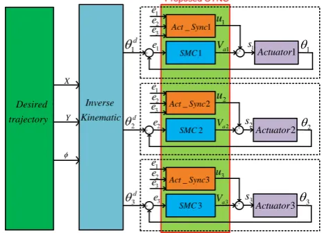
. By utilizing the inverse kinematic model presented in Section 2 to calculate the component reference profiles, a tracking controller is required to operate each component actuator to accomplish its given task. Nevertheless, in the parallel robots configuration and due to the model inaccuracy, system nonlinearities and uncertainties, the actuator operation without knowing the information from its neighbors could easily result in degradation of the end-effector performance or even make it unstable. To solve this problem, the synchronization controller is indispensable to compensate the error between the actuators and subsequently the overall robot performance can be significantly

improved.

Therefore, this paper proposes a schema control algorithm as shown in Fig. 4. Herein, three sliding mode control (SMC) modules are used to drive the component actuators to follow their desired trajectories while the three actuator synchronization modules (Act_Sync) are used to compensate the synchronization errors between these actuators. During the 3-RRR parallel robot operations, the actuator tracking errors are sent to the Act_Sync modules to evaluate the interaction between the actuators. The output from each Act_Sync is then added to the output of the corresponding SMC to drive its actuator to ensure the overall performance of the robot.

1

d



Inverse Kinematic X

1

SMC Actuator1

2

d



3

d

 Desired

trajectory Y



1  

_e1

2  



2

e

3  



3

e

1

a V

1 u

1

s

2

a

V 2 u

2 s

3

a V

3

u

3 s 2

SMC

3 SMC

2 Actuator

3 Actuator _ 1

Act Sync

2

e

3

e

1

e

_ 2

Act Sync

2

e1 e

3

e

_ 3

Act Sync

2

e

3

e

1

e

[image:4.595.312.546.209.377.2]

Proposed SYNC

Fig. 4 Proposed control scheme of 3-RRR parallel robot

3.1 Actuator controller design

In this section, the sliding mode controller is designed to ensure that each independent actuator could follow its given trajectory well. Without lost of generality, a DC motor driven actuator is selected for the control design. The mathematical model of the DC motor can be presented as.35,36

2

2

t a

d K b

i

dt J J

 _{  &} (5)

a a b a

a

a a a

di R K V

i

dt  L L L

& (6)

For a tracking reference of the motor, a sliding surface is defined as:



r



C r 

 &&   ₍₇₎ where_ris the position reference; C is a positive constant. Derivative of sliding surface is derived as

( ) K sign

&    (8)

where K is positive;

1 0

( ) 1 0

0 0

if

sign if

if



 

  



 _ 

 _



For stability analysis, the Lyapunov function is selected as follows:

2 1

1 2 V  

Talking derivative of this Lyapunov function, one has

2

1 . . 0

V& & K  

According to Lyapunov stability theorem, Eq. (8) is used to ensure the stability of the 3-RRR parallel robot.

[image:4.595.44.290.425.567.2]

r C r C

 

_& &&

 

& & &



(9) The term && can be obtained from Eqs. (5) and (6)

t a t a b t

a a

a a a

K L K R b K K

V i

R J R J R J

&&  &  & ₍₁₀₎

Therefore, Eq. (9) can be rewritten as

a b t t a t

r r a a

a a a

R b K K K L K

C C V i

R J R J R J

        

 

&& & & &

& (11)

Substitute Eq. (8) into the Eq. (11), the driving voltage from the SMC can be computed as

V

( )

a b t

r r

a a

a

t a t

a a

R b K K

C C

R J R J

K L K

i K sign

R J











                 _{ }        

&& & &

&

(12)

Assume that the angle and current DC motor are measured by the sensors. Eq. (12) can be calculated to configure the voltage for each actuator. In fact, the motors are often affected by the system uncertainties and disturbance. Therefore, the SMC cannot ensure the high accuracy. In the next section, the SYNC algorithm is presented to solve the shortcoming of SMC.

3.2 Synchronization controller design

The synchronization controller(SYNC) is used to compensate the error between the actuators. For design SYNC, the synchronization errors are defined as

 

t eA

 

t eB

 

t

   (13)

where e_A

   

t e, _B t are the actuators’ tracking errors, 

 

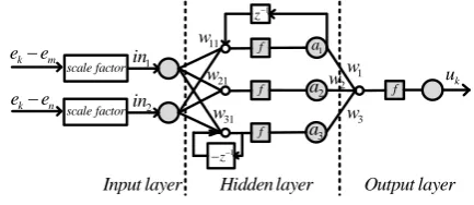
t is called the synchronization errors of SYNC.

The synchronization controller is then designed as the combination of the PID algorithm and a neural network. Structure of the PIDNNC is presented in Fig. 5.

1 in 2 in 11 w 21 w 31 w f f f 1 a 2 a 3 a

f uk

1 z 1 z  1 w 2 w 3 w

Input layer Hidden layer Output layer

k m

e e

k n

e e

[image:5.595.57.274.459.553.2]

scale factor scale factor

Fig. 5 Structure of PIDNNC

Here, the neural network includes an input layer, a hidden layer and an output layer. The input layer contains two input within range [-1 1] which are derived from the synchronization errors (ek-em)and (ek-en) by using scaling factors (ek , em , en are the tracking errors of kth _{, m}th _{and n}th

actuator, respectively; k,m,n

 

1 3; k ≠ m ≠ n). Using Eq. (13), the synchronization errors can be derived as

 

 

 

1 t e tk e tm



  (14)

 

 

 

2 t e tk e tn



  (15)

The input values of neural network can be defined as

 

2



 



1

j

j j

j j min

max min

in t



t















(16)

where

j j

j min max

 _{ }   are

th

j synchronization error ( j=1,2).

The hidden layer has three nodes which perform PID function. Therein, the 1st _{and 3}rd _{node use a delay factor z}-1 _{to perform the} integral and derivative terms while the 2nd _{node represents the} proportional term. The outputs of this layer can be computed by using the PID form as follows

 

   





 

   

 

   



 



2

1 1 1

1 2

2 2

1

2 2

3 3 3

1 1 1 1 1 j j j j j j

j j j j

j j

a t w t in t a t

a t w t in t

a t w t in t w t in t

           _         









(17)

wherewijare the weights of hidden layer



i1, 2,3 ; j1, 2



The output layer of the neural network has single node which is the adaptive control integrated to the control signal of each actuator to compensate the SYNC errors. By utilizing the PID algorithm, the network output is can be calculated as

 

3



   



1

k i i

i

u t w t a t







₍₁₈₎

wherew_iare the weights of output layer.

For updating the weights of the PIDNNC, back propagation algorithm37 _{is used to minimize the error between the desired input} and the output state of the robot system. Define an error function as:

 



 

 



₂



 

 



₂ 2

 

2 1

1 1 1

2 2 2

k k m k n j

j

E t e t e t e t e t  t



    



₍₁₉₎

where_j

 

t is synchronization error in Eqs. (14) and (15). In the step of time



t1



, the weights are turned using the back propagation learning algorithm as :



1



 

 

k

 

_{ }

ij ij ij

ij

E t

w t w t t

w t

 

  

 (20)

where_ij

 

t are the learning rates of the weightwijin the hidden

layer.

Using Eqs. (17),(18) and (19), one has

 

 

 

 

 

 

 

 

 

 

_{ }

   

2 1 2 1 j

k k k

j

ij j k ij

j

j i j

j k

y t

E t E t u t

w t y t u t w t

y t

t sgn w t in t u t         _  _        _{ }  _        _ _ _ __      





(21)

where y t₁

 

em

 

t ; y₂

 

t e tn

 

Therefore, the termw t_ij

 

is obtained from Eqs. (20) and (21)

 





 

 

 

 

_{ }

   

       

2 1 1

ij ij ij

j

ij j i j

j k

ij i j

w t w t w t

y t

t t sgn w t in t

u t

t p t w t in t

               _ _ _ __        



(22) where

 

2

 

 

_{ }

1

j j

j k

y t

p t t sgn

u t       _ _ __     



(23)

A Lyapunov function is defined as

 

2

 

2 2

1

1 2j j

V t  t







₍₂₄₎

DOI: XXX-XXX-XXXX obtained by

 





 







 



 

 



 



2 2 2

2 2 2

1 2 ₂ 1 1 1 1 2 1 2 j j j

j j j

j

V t V t V t t t

t t t

                 _    _  





₍₂₅₎

From Eq. (16), the term_j

 

t can be derived as

 



1



 

 

 

2

j j

max min

j t j t j t in tj Kj in tj

 

   

        (26)

where

2

j j

max min

j

K   (27)

Based on the structure of PIDNNC in Fig. 5, one has

 

2 3

 

_{ }

 

1 1

j

j il

l i il

in t

in t w t

w t        _ _  __     

 

(28)

Herein,

 

 

 

 

 

 

 

 

i

j il l

i

il ij

j

a t in t w t in t

a t

w t w t

in t   _  _    (29)

Substitute Eqs. (22) and (29) into Eq. (28),

 

 

_{         }

     

 

 

2 3 1 1 2 2 3 1 1 l

j il i l

l i ij

i l

il

l i ij

in t

in t t p t w t in t

w t

p t w t in t t w t              _ _ _           _ _ _    

 

 

(30)

Let

 

 

2



 



2

1

l l

q t p t in t







₍₃₁₎

By selecting the learning rates _ij

 

t as same as 

 

t . Eq. (30) becomes

 

 

_{ }

 



 



 

 

     

3 2 2 1 1 3 1 i j l

i ij l

i

i ij

w t

in t p t in t t

w t

w t

q t t w t       _{ }   _{  }        _ _  







(32)

Substitute Eq. (32) into Eq. (26),

 

3

 

_{     }

1

i

j j

i ij

w t

t K q t t

w t

 



 

  _ _





 (33)

Substitute Eq. (33) into Eq. (25),

 

 

 

_{     }

 

     

 

 

_{ }

   

 

 

   

3 2 1 2 2 3 1 1 2 3 1 1 2 2 3

2 2 2

1 1 1 2 1 2 i j j i ij j i j i ij i j j

j i ij

i j

j i ij

w t

t K q t t

w t V t

w t

K q t t

w t

w t

t K q t t

w t

w t

K q t t

w t                   _ _   _{ }             _ _ _ _   _{   }          _ _ _      _{ }     _ _  _{ }   















By using Lyapunov stability theorem, the stability of the closed-loop control system using the PIDNNC is guaranteed if V t2

 

0. The learning rate

 

t can be chosen by

 

 

 

_{ }

 

 

 

2 3 1 1 2 2 3 2 1 1 i j j

j i ij

i j

j i ij

w t t K

w t t

w t

K q t

w t           _ _  _{ }      _{ }   _{ }     _{ }   









(34)

[image:6.595.296.554.190.566.2]

Eq. (34) is essential for the stability of the system. Therefore, by regulating online the learning rate to satisfy Eq. (34), the SYNC errors can be asymptotically converged to zeros and therefore, the system is stable.

Fig. 6 Simulation model of 3-RRR parallel robot

4. Numerical simulations

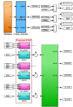
In this section, simulations have been carried out to evaluate the performance of the 3-RRR parallel robot using the proposed control approach.

First, a simulation model based on Solidwork and Matlab/Simulink was constructed as in Fig. 6. Herein, the 3D model of the robot was drawn in Solidwork and then the SimMechanics Link exporter toolbox was used to create the dynamic models from the 3D model for a capable of visualizing the system operation with the desired inputs and outputs in the Simulink environment.

[image:7.595.302.549.93.271.2]

parameters were properly selected from the experimental setup38 and the geometry dimensions of 3-RRR parallel robot were given in the analysis of manipulator.19

Table 1 Setting parameters for the 3-RRR parallel robot

Component Specification Value

Geometry

Length of first link 400mm Length of second link 600mm Dimension of the moving

platform

350mm

DC motor

t

K 0.0302Nm/A

b

K 0.0946V/rad/s

b 1.34e-5N.m.s

J 1.34e-5kgm2

a

R 0.316

a

L 0.00008H

Mass

First link 0.8kg

Second link 1.2kg

Moving platform 1.5kg

Second, the control algorithms were added to the developed model to drive the moving platform to track any desired trajectories. For a comparative study, the proposed control approach was presented in Section 3 and Fig. 4 (denoted as SYNC2) has been investigated with other two controllers which are a non-synchronization controller slide mode controller (denoted as NONSYNC) and a synchronization ANFIS-based fuzzy controller (denoted as SYNC1)2_.

The SYNC2 was implemented based on the design procedure introduced in Section 3 in which the gain for the sliding surface (Section 3.1) was chosen as K=10 and C=2 while the initial weights of synchronization control module (Section 3.2) were set as wi=1; wjk=0.1; (i,j=1,2,3; k=1,2). The NONSYNC was constructed as the three independent SMC controllers of the SYNC2 while the SYNC1 control structure and its parameters were designed and initialized based on the results from the previous study2_.

For the simulations, initial position of the moving platform was defined as x=0.5; y=0.35;



0; a reference trajectory of the moving platform is given as follows:

0.5 0.03 3

x  cos_



t_

 

0.35 0.03 3 y  sin_t_

 

0





where t is the simulation time; ( t=kt; t 0.01s; k=0, 1, 2 ...). By using the inverse kinematic model of the 3-RRR planar parallel robot derived in Section 2, the desired angle for each actuator can be computed based on the reference trajectory of the moving platform. In order to assess the capability of the compared controllers, different working conditions of the simulated system were generated by using two test cases established in Table 2. For the test cases 2, the disturbances were represented as load torques

[image:7.595.47.294.115.309.2]

which were externally added to the actuators as plotted in Fig. 7. Each simulations was then performed for a period of 6 seconds.

Table 2 Simulation test cases

Number of cases Content

1 Ideal condition - No disturbance 2 All of actuator have the disturbances

0 1 2 3 4 5 6

-1.0 -0.5 0.0 0.5 1.0

Load t

orque

(N

m

)

Time (s)

Added disturbance at joint 1 Added disturbance at joint 2 Added disturbance at joint 3

Fig. 7 Disturbance generation for 3-RRR parallel robot

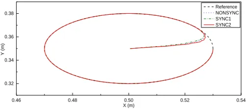
By employing the test case 1, the control tests were performed in the ideal condition to assess the actuators’ controller. As the result in Fig. 8(a), the moving platform could track accurately the desired trajectory by using any of the compared controllers. This indicates that the inverse kinematic model was well established to compute the targeted profiles for the actuators and the actuator controllers were properly designed to enhance their given tasks. The tracking results of the robot actuators were analyzed in Figs. 8(b) to 8(d). The system using the SYNC1 reached the stable performances lightly slower than those using the NONSYNC and SYNC2 (Fig. 8(b) and Fig. 8(c)). The reason was that the SYNC1 employed the fuzzy and ANFIS control modules to enhance the actuator tracking control and synchronization control, respectively. And both of these control modules needed more time to adjust their parameters during the operation to adapt to the working conditions. While the performance of the NONSYNC and SYNC2 were quite similar due to the same SMC use. By using the SYNC2 with the advanced control in which the learning rate was adaptively adjusted, the component actuators could follow well their paths (given by inverse kinematic model ) with the errors converged to zeros in the shortest times as depicted in Fig. 8(b) and Fig. 8(c). Due to working in the ideal condition, the sync errors reached to zeros simultaneously as well as the actuator errors (see Fig. 8(d)).

0.46 0.48 0.50 0.52 0.54

0.32 0.34 0.36 0.38

Y

(m

)

X (m)

Reference NONSYNC SYNC1 SYNC2

[image:7.595.307.558.624.735.2]

DOI: XXX-XXX-XXXX 2.10 2.15 2.20 2.25 2.30 Jo int 1 (r a d

) Reference _NONSYNC

SYNC1 SYNC2 3.9 4.0 4.1 Jo int 2 (r a d )

0 1 2 3 4 5 6

0.1 0.2 0.3 0.4 Jo int 3 (r a d ) Time (s) (b) Performance of actuators

0.00 0.05 0.10 Err o r Traj Jo int 1 (r a d

) NONSYNC

SYNC1 SYNC2 -0.01 0.00 0.01 Err o r Traj Jo int 2 (r a d )

0 1 2 3 4 5 6

-0.10 -0.05 0.00 0.05 Err o r Traj Jo int 3 (r a d ) Time (s)

(c) Trajectory errors of actuators

-0.10 -0.05 0.00 Syn c e rr o r e 12 (r a d ) NONSYNC SYNC1 SYNC2 -0.10 -0.05 0.00 0.05 0.10 Syn c e rr o r e 23 (r a d )

0 1 2 3 4 5 6

[image:8.595.44.564.60.649.2]

0.0 0.1 0.2 Syn c e rr o r e 31 (r a d ) Time (s) (d) Synchronization errors

Fig. 8 Response of 3-RRR parallel robot without disturbance using difference controllers

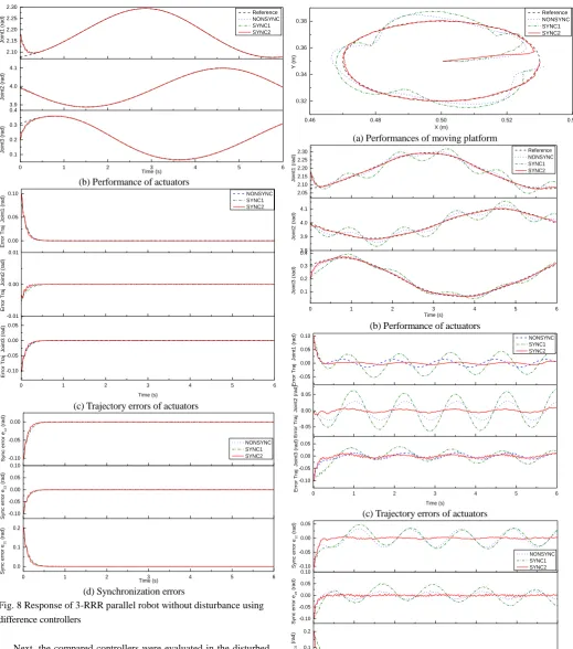
Next, the compared controllers were evaluated in the disturbed condition generated from the second test case. As displayed in Fig. 7, the actuators were influenced by three disturbances sources which were the sinusoidal signals with different frequencies. Furthermore, white noises were added to the first source to represent the actual working environment. Subsequently, the result obtained in Fig. 9(a) showed that the moving platform could not reach the desired goal by using the NONSYNC due to the lack of control compensation between the component actuators. The

0.46 0.48 0.50 0.52 0.54

0.32 0.34 0.36 0.38 Y (m ) X (m) Reference NONSYNC SYNC1 SYNC2

(a) Performances of moving platform

2.05 2.10 2.15 2.20 2.25 2.30 Jo int 1 (r a d

) Reference _NONSYNC

SYNC1 SYNC2 3.8 3.9 4.0 4.1 Jo int 2 (r a d )

0 1 2 3 4 5 6

0.1 0.2 0.3 0.4 Jo int 3 (r a d ) Time (s)

(b) Performance of actuators

-0.05 0.00 0.05 0.10 E rr o r Traj Jo int 1 (r a d ) NONSYNC SYNC1 SYNC2 -0.05 0.00 0.05 E rr o r Traj Jo int 2 (r a d )

0 1 2 3 4 5 6

-0.10 -0.05 0.00 0.05 E rr o r Traj Jo int 3 (r a d ) Time (s)

(c) Trajectory errors of actuators

-0.10 -0.05 0.00 0.05 Syn c e rr o r e 12 (r a d ) NONSYNC SYNC1 SYNC2 -0.10 -0.05 0.00 0.05 0.10 Syn c e rr o r e 23 (r a d )

0 1 2 3 4 5 6

0.0 0.1 0.2 Syn c e rr o r e 31 (r a d ) Time (s)

[image:8.595.297.553.97.712.2]

(d) Synchronization errors

disturbances caused unwanted impacts on the actuators(Fig. 9(b)(c)(d)). The SYNC1 with the synchronization between the actuators could not guaranteed the tracking performance, so that there existed large errors along the trajectory. The reason was there was no stability condition in the ANFIS-based synchronization design and updating mechanism. This led to the requirement to train the ANFIS before the utilization in order to achieve the higher control accuracy. Meanwhile, the SYNC2 could ensure the good tracking with remarkably small errors (Fig. 9(c)(d)). This came as no surprise because the proposed control scheme processes not only the adaptive actuator controllers but also the adaptive synchronization mechanism. The PIDNNC with the dynamic learning rate, regulated by the Lyapunov stability constraints allowed the system to response quickly to any changes. Consequently, the disturbances could be compensated effectively(Fig. 9(a)(b)). The result proved convincingly that the robot performance in terms of speed and accuracy could be maintained by employing the proposed control approach for the environment containing large noises and disturbances.

5. Conclusions

This paper presents the advanced synchronization controller to deal with the tracking problem of the 3-RRR parallel robot. The proposed controller is excellent combination of the two control techniques SMC and PIDNNC. Herein, the SMC is designed for each actuator to track the given trajectory while the PIDNNC-based synchronization controller is used to compensate the errors between actuators caused by noises and disturbances. As a result, the moving platform can track the desired target quickly with high accuracy even in the bad working conditions. The effectiveness of the proposed control method has been evidently provided through the series of comparisons with the other controllers in operating the 3-RRR robot by mean of simulations.

As the future work, an experimental 3-RRR parallel robot is now constructing for evaluating the control ability. Further research on how to improve the adaptation and tracking accuracy of the proposed control algorithm will be also considered as a next step.

REFERENCES

1. Balan, R., Maties, V., Stan, S., and Lapusan, C., “On the Control of a 3-RRR Planar Parallel Minirobot,” Journal of Romanian Society of Mechatronics, No. 4, pp. 20-23, 2005. 2. Khoa, L, D., Truong, D, Q., and Ahn, K, K., “Synchronization

controller for a 3-R planar parallel pneumatic artificial muscle (PAM) robot using modified ANFIS algorithm,” Mechatronics, Vol. 23, No. 4, pp. 462-479, 2013.

3. Lorena, S, F., and Carvalho, J, C, M., “Using the planar 3-RRR parallel manipulator for rehabilitation of human hand,” ABCM Symposium Series in Mechatronics, Vol. 6, pp. 535-542, 2014.

4. Guilherme, D, F., ClodoaldoSchutel, F, N., and Alexandre, C., “A servo controlled 3-RRR parallel robot operation modes and workspace safety,” 23rd ABCM International Congress of Mechanical Engineering, 2015.

5. Yong, L, K., Tsu, P, L., and Chun, Y, W., “Experimental and Numerical Study on the Semi-Closed Loop Control of a Planar Parallel Robot Manipulator,” Mathematical Problems in Engineering, 2014.

6. Ketankumar, H, P., Vinit, C, N., Yogin, K, P., and Patel Y, D., “Workspace and singularity analysis of 3-RRR planar parallel manipulator,” Proceeding of the 1st _{International and 16}th National Conference on Machines and Mechanisms, 2013. 7. Azadeh, D., Mohsen, H., Mehdi, T, M., and Masume, M, E., “An

experimental study on open-loop position and speed control of a 3-RRR planar parallel mechanism,” RSI International Conference on Robotics and Mechatronics, pp. 176-181, 2015.

8. Shao, Z., Tang, X., Chen, X., and Wang, L., “Inertia Match of a 3-RRR Reconfigurable Planar Parallel Manipulator,” Chinese Journal of Mechanical, Vol. 22, No. 6, pp. 791-799, 2009. 9. Jung, H, C., Tae, W, S., and Jeh, W, L., “Singularity Analysis of

a Planar Parallel Mechanism with Revolute Joints based on a Geometric Approach,” Int. J. Precis. Eng. Manuf., Vol. 14, No. 8, pp. 1369-1375, 2013.

10.Staicu, S., “Kinematics of the 3-RRR planar parallel robot,” Mechanical Engineering, Vol.70, No. 2, pp. 3-14, 2008. 11.Xuchong, Z., and Xianmin, Z., “A comparative study of planar

3-RRR and 4-RRR mechanisms with joint clearances,” Robotics and Computer-Integrated Manufacturing, Vol. 40, pp. 24-33, 2016.

12.Robert, L, W., and Brett, H, S., “Inverse kinematics for planar parallel manipulators,” ASME Design Technical Conferences, 1997.

13.Hamdoun, O., Baghli, F, Z., and Bakkali, L, E., “Inverse kinematic Modeling of 3RRR Parallel Robot,” French Congress of Mechanics Lyon, 2015.

14.Hamed, S, B., and Javad, E., “Direct Kinematics Solution of 3-RRR Robot by Using two difference Artificial Neural Network,” RSI International Conference on Robotics and Mechatronics, 2015.

15.Santos, J, C., Rocha, D, M., and Silva, M, M., “Performance evaluation of Kinematically redundant planar parallel manipulators,” ABCM Symposium Series in Mechatronics, Vol. 6, 2014.

16.Miguel, A, T., Garrido, R., and Alberto, S., “Stable Visual PID Control of Redundant Planar Parallel Robots,” InTech., pp. 27-50, 2011.

DOI: XXX-XXX-XXXX

18.Niu, X., G, Gao., Xinjun, L., and Zhiming, F., “Decoupled Sliding Mode Control for a Novel 3-DOF Parallel Manipulator with Actuation Redundancy,” Int. J. Advanced Robotic Systems, Vol. 12, No. 5, 2015.

19.Amin, N., Musa, M., and Ali Z., “Intelligent active force control of a 3-RRR parallel manipulator incorporating fuzzy resolved acceleration control,” Mathematical Modelling, Vol. 36, pp. 2370-2383, 2012.

20.Amin, N., Musa, M., and Ali, Z., “Active Force Control of 3-RRR Planar Parallel Manipulator,” International Conference on Mechanical and Electrical Technology, pp. 77-81, 2010. 21.Noshadi, A., and Mailah, M., “Active disturbance rejection

control of a parallel manipulator with self learning algorithm for a pulsating trajectory tracking task,” Mechanical Engineering, Vol. 19, No. 1, pp. 132-141, 2012.

22.Weiwei, S., and Shuang, C., “Nonlinear computed torque control for a high-speed planar parallel manipulator,” Mechatronics, Vol. 19, pp. 987-992, 2009.

23.Varalakshmi, K,V., and Srinivas, D, J., “Nonlinear Tracking Control of Parallel Manipulator Dynamics with Intelligent Gain Tuning Scheme,” Int. J. Mechanical, Electrical and Computer Technology, Vol. 6, pp. 2932-2942, 2016.

24.Shang, W., and Cong, S., “Robust nonlinear control of a planar 2-DOF parallel manipulator with redundant actuator,” Robotics and Computer-Integrated Manufacturing, Vol. 30, No. 6, pp. 597-604, 2014.

25.Su, Y., Sun, D., Ren, L., and Mills, K., “Integration of Saturated PI Synchronous Control and PD feedback for control of Parallel Manipulators,” IEEE Transaction on Robotics, Vol. 22, No. 1, pp. 202-207, 2006.

26.Su, Y, X., and Sun, D., “A Model Free Synchronization Approach to Controls of Parallel Manipulators,” International Conference on Robotics and Biomimetics, 2004.

27.Lu, R., James, K, M., and Dong, S., “Trajectory Tracking Control for a 3-DOF Planar parallel manipulator using the convex synchronized control method,” IEEE Transactions on Control Systems Technology, Vol. 16, No. 4, pp. 613-623, 2008. 28.Jung, H, B., “A Method of Synchronous Control System for Dual Parallel Motion Stages,” Int. J. Precis. Eng. Manuf., Vol. 13, No. 6, pp. 883-889, 2012.

29.Seung, H, C., “Trajectory Tracking Control of a Pneumatic XY Table Using Neural Network Based PID Control,” Int. J. Precis. Eng. Manuf., Vol. 10, No. 5, pp. 37-44, 2009.

30.Lu, R., James, K, M., and Dong, S., “Performance Improvement of Tracking Control for a Planar Parallel Robot Using Synchronized Control,” IEEE/RSJ International Conference on Intelligent Robots and Systems, pp. 2539-2544, 2006.

31.Lu, R., James, K, M., and Dong, S., “Adaptive Synchronization

Control of a Planar Parallel Manipulator,” Proceedings of the 2004 American Control Conference, Vol. 5, pp. 3980-3985, 2004.

32.Lu, R., James, K, M., and Dong, S., “Adaptive Synchronized Control for a Planar Parallel Manipulator Theory and Experiments,” Journal of Dynamic Systems, Measurement, and Control, Vol. 128, No. 4, pp. 976-979, 2005.

33.Su, Y, X., and Sun, D., “Nonlinear PD Synchronized Control for parallel manipulators,” Proceedings of the 2005 IEEE International Conference on Robotics and Automation, 2005. 34.Shih, M, W., Ren, J,W., and Shambaljamts, T., “A New

Synchronous Error Control Method for CNC Machine Tools with Dual-Driving Systems,” Int. J. Precis. Eng. Manuf., Vol. 14, No. 8, pp. 1415-1419, 2013.

35.Barna, G.,“Simulation Model of a Series DC Motor for Traction Rail Vehicle,” Int. Conference on Methods and Models in Automation and Robotics, pp. 531-536, 2016.

36.Esen, Z, I., Cakroglu, S., Sahin, M., and Kulunk, Z., “Modeling, Simulation and Validation of DC Motor with spring load system,” IEEE Int. Power Electronics and Motion Control Conference, pp. 732-736, 2016.

37.Reed, R, D., and Marks, R, .J., “Neural Smithing - Supervised Learning in Feedforward Artificial Neural Networks,” MIT Press Camebridge MA, 1998.