Weakly informative reparameterizations for location scale mixtures

warwick.ac.uk/lib-publications

Original citation:

Kamary, Kaniav, Lee, Jeong Eun and Robert, Christian P. (2018) Weakly informative reparameterizations for location-scale mixtures. Journal of Computational and Graphical Statistics. doi:10.1080/10618600.2018.1438900

Permanent WRAP URL:

http://wrap.warwick.ac.uk/103040

Copyright and reuse:

The Warwick Research Archive Portal (WRAP) makes this work by researchers of the University of Warwick available open access under the following conditions. Copyright © and all moral rights to the version of the paper presented here belong to the individual author(s) and/or other copyright owners. To the extent reasonable and practicable the material made available in WRAP has been checked for eligibility before being made available.

Copies of full items can be used for personal research or study, educational, or not-for profit purposes without prior permission or charge. Provided that the authors, title and full bibliographic details are credited, a hyperlink and/or URL is given for the original metadata page and the content is not changed in any way.

Publisher’s statement:

“This is an Accepted Manuscript of an article published by Taylor & Francis Journal of Computational and Graphical Statistics on 13/02/2018 available online

https://doi.org/10.1080/10618600.2018.1438900

A note on versions:

The version presented here may differ from the published version or, version of record, if you wish to cite this item you are advised to consult the publisher’s version. Please see the ‘permanent WRAP URL’ above for details on accessing the published version and note that access may require a subscription.

Weakly informative reparameterisations for

location-scale mixtures

Kaniav Kamary

Universit´

e Paris-Dauphine, CEREMADE, and INRIA, Saclay

Jeong Eun Lee

Auckland University of Technology, New Zealand

and

_{Christian P. Robert}

Universit´

e Paris-Dauphine, and University of Warwick

August 1, 2017

Abstract

While mixtures of Gaussian distributions have been studied for more than a cen-tury, the construction of a reference Bayesian analysis of those models remains un-solved, with a general prohibition of improper priors (Fr¨uhwirth-Schnatter, 2006) due to the ill-posed nature of such statistical objects. This difficulty is usually bypassed by an empirical Bayes resolution (Richardson and Green, 1997). By creating a new parameterisation centred on the mean and possibly the variance of the mixture distri-bution itself, we manage to develop here a weakly informative prior for a wide class of mixtures with an arbitrary number of components. We demonstrate that some poste-rior distributions associated with this pposte-rior and a minimal sample size are proper. We provide MCMC implementations that exhibit the expected exchangeability. We only study here the univariate case, the extension to multivariate location-scale mixtures being currently under study. An R package called Ultimixt is associated with this paper.

Keywords: Non-informative prior, improper prior, mixture of distributions, Bayesian anal-ysis, Dirichlet prior, exchangeability, polar coordinates, compound distributions.

∗_{Kaniav Kamary and Christian Robert, CEREMADE, Universit´e Paris-Dauphine, 75775 Paris cedex}

16, France, kamary,[email protected], Jeong Eun Lee, Auckland University of Technology, New Zealand,[email protected]. The authors are grateful to Robert Kohn for his helpful comments and to all reviewers for improving the presentation of the paper.

1

Introduction

A mixture density is traditionally represented as a weighted average of densities from standard families, i.e.,

f(x|θ,p) =

k

X

i=1

pifi(x|θi)

k

X

i=1

pi = 1. (1)

Each component of the mixture is characterised by a component-wise parameterθi and the

weights pi of those components translate the importance of each of those components in

the model. A more general if rarely considered mixture model involves different families for the different components.

This particular representation 1 gives a separate meaning to each component through its parameter θi, even though there is a well-known lack of identifiability in such models,

due to the invariance of the sum by permutation of the indices. This issue relates to the equally well-known “label switching” phenomenon in the Bayesian approach to the model, which pertains both to Bayesian inference and to simulation of the corresponding posterior (Celeux et al., 2000; Stephens, 2000b; Fr¨uhwirth-Schnatter, 2001; Jasra et al., 2005). From this Bayesian viewpoint, the choice of the prior distribution on the component parameters is quite open, the only constraint being obviously that the corresponding posterior is proper. Diebolt and Robert (1994) and Wasserman (1999) discussed the alternative approach of imposing proper posteriors on improper priors by banning almost empty components from the likelihood function. While consistent, this approach induces dependence between the observations, requires a large enough number of observations, higher computational costs, and does not handle over-fitting very well.

The prior distribution on the weightspiis equally open for choice, but a standard version

is a Dirichlet distribution with common hyperparameter α0, Dir(α0, . . . , , α0). Recently,

Rousseau and Mengersen (2011b) demonstrated that the choice of this hyperparameter α0

relates to the inference on the total number of components, namely that a small enough value of α0 manages to handle over-fitted mixtures in a convergent manner. In Bayesian

non-parametric modelling, Griffin (2010) showed that the prior on the weights may have a higher impact when inferring about the number of components, relative to the prior on the component-specific parameters. As indicated above, the prior distribution on the θi’s has

received less attention and conjugate choices are most standard, since they facilitate simu-lation via Gibbs samplers (Diebolt and Robert, 1990; Escobar and West, 1995; Richardson and Green, 1997) if not estimation, since posterior moments remain unavailable in closed form. In addition, Richardson and Green (1997) among others proposed data-based priors that derive some hyperparameters as functions of the data, towards an automatic scaling of such priors, as illustrated by the R package, bayesm (Rossi and McCulloch, 2010).

has been done, apart from Bernardo and Gir`on (1988), who derived the Jeffreys priors for mixtures where components have disjoint supports, Figueiredo and Jain (2002) who used independent Jeffreys prior on components, and Rubio and Steel (2014) which achieve a closed-form expression for the Jeffreys prior of a location-scale mixture with two disjoint components. Recently, Grazian and Robert (2015) undertook an analytical and numerical study of Jeffreys priors for Gaussian mixtures, which showed that Jeffreys priors are almost invariably associated with improper posteriors, whatever the sample size, and advocated the use of pseudo-priors expressed as conditional Jeffreys priors for each type of parameters. In this paper, we instead start from the traditional Jeffrey prior for a location-scale parameter to derive a joint prior distribution on all parameters by taking advantage of compact reparameterisation, which allow for uniform distributions and similarly weakly informative distributions.

In the case when θi = (µi, σi) is a location-scale parameter, Mengersen and Robert

(1996) have already proposed a reparameterisation of (1) that express each component as a local perturbation of the previous one, namely µi = µi−1 +σi−1δi, σi = τiσi−1, τi < 1

(i >1), withµ1 andσ1being the reference values. Based on this reparameterisation, Robert

and Titterington (1998) established that a specific improper prior on (µ1, σ1) leads to a

proper posterior in the Gaussian case. We propose here to modify this reparameterisation by using the mean and variance of the mixture distribution as reference location and scale, respectively. This modification has foundational consequences in terms of identifiability and hence of exploiting improper and non-informative priors for mixture models, in sharp contrast with the existing literature (see, e.g. Diebolt and Robert, 1994; Wasserman, 1999). Computational approaches to Bayesian inference on mixtures are quite diverse, start-ing with the introduction of the Gibbs sampler (Diebolt and Robert, 1990; Gelman and King, 1990; Escobar and West, 1995), some concerned with approximations (Roeder, 1990; Wasserman, 1999) and MCMC features (Richardson and Green, 1997; Celeux et al., 2000), and others with asymptotic justifications, in particular when over-fitting mixtures (Rousseau and Mengersen, 2011b), but most attempting to overcome the methodological hurdles in estimating mixture models (Chib, 1995; Neal, 1999; Berkhof et al., 2003; Marin et al., 2005; Fr¨uhwirth-Schnatter, 2006; Lee et al., 2009). While we do not propose here a novel compu-tational methodology attached with our new priors, we study the performances of several MCMC algorithms on such targets.

2

Mixture reparameterisation

2.1

Mean and variance of a mixture

Let us first recall how both mean and variance of a mixture distribution with finite first two moments can be represented in terms of the mean and variance parameters of the components of the mixture.

Lemma 1 If µi and σ2i are well-defined as mean and variance of the distribution with

density fi(·|θi), respectively, the mean of the mixture distribution (1) is given by

Eθ,p[X] =

k

X

i=1

piµi

and its variance by

varθ,p(X) =

k

X

i=1

piσ2i + k

X

i=1

pi(µ2i −Eθ,p[X]2)

For any location-scale mixture, we propose a reparameterisation of the mixture model that starts by scaling all parameters in terms of its global meanµand global variance1 _σ2_.

For instance, we can switch from the parameterisation in (µi, σi) to a new parameterisation

in (µ, σ, α1, . . . , αk, τ1, . . . , τk, p1, . . . , pk),expressing those component-wise parameters as

µi =µ+σαi and σi =στi 1≤i≤k (2)

where τi > 0 and αi ∈ R. This bijective reparameterisation is similar to the one in

Mengersen and Robert (1996), except that these authors put no special meaning on their location and scale parameters, which are then non-identifiable. Once µand σ are defined as (global) mean and variance of the mixture distribution, eqn. (2) imposes compact constraints on the other parameters of the model. For instance, since the mixture variance is equal to σ2, this implies that (µ1, . . . , µk, σ1, . . . , σk) belongs to an ellipse conditional on

the weights, µ, and σ, by virtue of Lemma 1.

Considering theαi’s and theτi’s in (2) as the new and local parameters of the mixture

components, the following result (Lemma 2) states that the global mean and variance pa-rameters are the sole freely varying papa-rameters. In other words, once both the global mean and variance are defined as such, there exists a parameterisation such that all remaining parameters of a mixture distribution are restricted to belong to a compact set, a feature that is most helpful in selecting a non-informative prior distribution.

Lemma 2 The parameters αi and τi in (2) are constrained by

k

X

i=1

piαi = 0 and k

X

i=1

piτi2+ k

X

i=1

piα2i = 1.

1_{Strictly speaking, the termglobalis superfluous, but we add it nonetheless to stress that those moments}

The same concept applies for other families, namely that one or several moments of the mixture distribution can be used as a pivot to constrain the component parameters. For instance, a mixture of exponential distributionsE(λ−_i 1) or a mixture of Poisson distributions

P(λi) can be reparameterised in terms of its mean, E[X], through the constraint

E[X] =λ=

k

X

i=1

piλi,

by introducing the parameterisation λi = λγi/pi, γi > 0, which implies

Pk

i=1γi = 1. As

detailed below, this notion immediately extends to mixtures of compound distributions, which are scale perturbations of the original distributions, with a fixed distribution on the scales.

2.2

Proper posteriors of improper priors

The constraints in Lemma 2 define a set of values of (p1, . . . , pk, α1, . . . , αk, τ1, . . . , τk) that

is obviously compact. One sensible modelling approach exploiting this feature is to resort to uniform or other weakly informative proper priors for those component-wise parameters, conditional on (µ, σ). Furthermore, since (µ, σ) is a location-scale parameter, we invoke Jeffreys (1939) to choose a Jeffreys-like priorπ(µ, σ) = 1/σon this parameter, even though we stress this is not the genuine (if ineffective) Jeffreys prior for the mixture model (Grazian and Robert, 2015). In the same spirit as Robert and Titterington (1998), we now establish that this choice of prior produces a proper posterior distribution for a minimal sample size of two.

Theorem 1 The posterior distribution associated with the prior π(µ, σ) = 1/σ and with the likelihood derived from (1) is proper when the components f1(·|µ, σ), . . . , fk(·|µ, σ) are

Gaussian densities, provided (a) prior distributions on the other parameters are proper and independent of (µ, σ), and (b) there are at least two observations in the sample.

While only handling the Gaussian case is a limitation, the above result extends to mixtures of compound Gaussian distributions, which are defined as scale mixtures, namely X =µ+σξZ, Z ∼N(0,1) and ξ ∼h(ξ), whenh is a probability distribution on_R+ _with

second moment equal to 1. (The moment constraint ensures that the mean and variance of this compound Gaussian distribution areµandσ2, respectively.) As shown by Andrews and Mallows (1974), by virtue of Bernstein’s theorem, such compound Gaussian distributions are identified as completely monotonous functions and include a wide range of probability distributions like the t, the double exponential, the logistic, and the α-stable distributions (Feller, 1971).

Corollary 1 The posterior distribution associated with the prior π(µ, σ) = 1/σ and with the likelihood derived from (1) is proper when the component densities fi(·|µ, σ) are all

The proof of this result is a straightforward generalisation of the one of Theorem 1, which involves integrating out the compounding variables ξ1 and ξ2 over their respective

distributions. Note that the mixture distribution (1) allows for different classes of location-scale distributions to be used in the different components.

If we now consider the case of a Poisson mixture,

f(x|λ1, . . . , λk) =

1 x!

k

X

i=1

piλxie

−λi ₍₃₎

with a reparameterisation as λ = _E[X] and λi = λγi/pi, we can use the equivalent to

the Jeffreys prior for the Poisson distribution, namely, π(λ) = 1/λ, since it leads to a well-defined posterior with a single positive observation.

Theorem 2 The posterior distribution associated with the prior π(λ) = 1/λ and with the Poisson mixture (3) is proper provided (a) prior distributions on the other parameters are proper and independent of λ and, (b) there is at least one strictly positive observation in the sample.

Once again, this result straightforwardly extends to mixtures of compound Poisson distributions, namely distributions where the parameter is random with mean λ:

P(X =x|λ) =

Z ₁

x!(λξ)

x_{exp{−λξ}dν(ξ),}

with the distribution ν possibly discrete. In the special case whenν is on the integers, this representation covers all infinitely exchangeable distributions (Feller, 1971).

Corollary 2 The posterior distribution associated with the priorπ(λ) = 1/λ and with the likelihood derived from a mixture of compound Poisson distributions is proper provided (a) prior distributions on the other parameters are proper and independent to λ and, (b) there is at least one strictly positive observation in the sample.

Another instance of a proper posterior distribution is provided by exponential mixtures,

f(x|λ1, . . . , λk) = k

X

i=1

pi

λi

e−x/λi_{, (4)}

since a reparameterisation via λ = _E[X] and λi = λγi/pi leads to the posterior being

well-defined for a single observation.

Theorem 3 The posterior distribution associated with the prior π(λ) = 1/λ and with the likelihood derived from the exponential mixture (4) is proper provided proper distributions are used on the other parameters.

Once again, this result directly extends to mixtures of compound exponential distribu-tions, namely exponential distributions where the parameter is random with mean λ:

f(x|λ) = Z

1

λξexp{−

In particular, this representation contains all Gamma distributions with shape less than one (Gleser, 1989) and Pareto distributions (Klugman et al., 2004).

Corollary 3 The posterior distribution associated with the priorπ(λ) = 1/λ and with the likelihood derived from a mixture of compound exponential distributions is proper provided proper distributions are used on the other parameters.

The parameterisation (2) is one of many of a Gaussian mixture. In practice, one could design a normal and a inverse-gamma distribution as priors for αi and τi, respectively, and

make those priors vague via the choice of hyperparameters derived from the standardised data (borrowing the idea by Rossi and McCulloch (2010)). This would make the prior on local parameters a data-based prior and consequently the marginal prior for µi and

σi would also be a data-based prior. A fundamental difficulty with this scheme is that

the constraints found in Lemma 2 are incompatible with this independent modelling to each other. We are thus seeking another parameterisation of the mixture that allows for a natural and weakly informative prior (hence not based on the data) while incorporating the constraints. This is the purpose of the following sections.

2.3

Further reparameterisations in location-scale models

We are now building a reparameterisation that will handle the constraints of Lemma 2 in such a way as to allow for manageable uniform priors on the resulting parameter set. Exploiting the form of the constrains, we can rewrite the component location and scale parameters in (2) as αi =γi/

√

pi and τi =ηi/

√

pi,leading to the mixture representation

f(x|θ,p) =

k

X

i=1

pifi(x|µ+σγi/

√

pi, σηi/

√

pi), ηi >0, (5)

Given the weight vector (p1,· · · , pk), these new parameters are constrained by k

X

i=1 √

piγi = 0 and k

X

i=1

(η_i2+γ_i2) = 1, (6)

which means that (γ1, . . . , γk, η1, . . . , ηk) belongs both to a hyper-sphere of R2k and to a

hyperplane of this space, hence to the intersection between both. Since the supports of ηi

and γi are bounded (i.e., 0≤ ηi ≤ 1 and −1 ≤ γi ≤ 1), any proper distribution with the

appropriate support can be used as prior and extracting knowledge from the data is not necessary to build vague priors as in Richardson and Green (1997).

Given these new constraints, the parameter set remains complex and the ensuing con-struction of a prior still is delicate. We can however proceed towards Dirichlet style distri-butions on the parameter. First, mean and variance parameters in (5) can be separated by introducing a supplementary parameter, namely a radius ϕsuch that

k

X

i=1

γ_i2 =ϕ2 and

k

X

i=1

This decomposition of the spherical constraint then naturally leads to a hierarchical prior where, for instance, ϕ2 _{and (p}

1, . . . , pk) are distributed as Be(a1, a2) and Dir(α0, . . . , α0)

variates, respectively, while the vectors (γ1, . . . , γk) and (η1, . . . , ηk) are uniformly

dis-tributed on the spheres of radius ϕand p1−ϕ2_{, respectively, under the additional linear}

constraint Pk

i=1 √

piγi = 0.

Since this constraint is an hindrance for easily simulating the γi’s, we now complete

the move to a new parameterisation, based on spherical coordinates, which can be handled most straightforwardly.

2.3.1 Spherical coordinate representation of the γ’s

In equations (6), the vector (γ1, . . . , γk) belongs both to the hyper-sphere of radius ϕ and

to the hyperplane orthogonal to (√p1, . . . , √

pk). Therefore, (γ1, . . . , γk) can be expressed

in terms of its spherical coordinates within that hyperplane. Namely, if (_z1, . . . ,zk−1)

denotes an orthonormal basis of the hyperplane, (γ1, . . . , γk) can be written as

(γ1, . . . , γk) = ϕcos($1)z1+ϕsin($1) cos($2)z2+. . .+ϕsin($1)· · ·sin($k−2)zk−1

with the angles $1, . . . , $k−3 in [0, π] and $k−2 in [0,2π]. The s-th orthonormal base zs

can be derived from the k-dimensional orthogonal vectors zes where

e

z1,j =

( −√p

2, j = 1

√

p1, j = 2

0, j >2

and the s-th vector is given by (s >1)

e

zs,j =

    

   

−(pjps+1)1/2

. Xs l=1pl

1/2

, j ≤s Xs

l=1pl

1/2

, j =s+ 1

0, j > s+ 1

Note the special case when k = 2 when the angle $1 is missing. In this case, the

mixture location parameter is then defined by (γ1, γ2) = ϕz1 and ϕ takes both positive

and negative values. In the general case, the parameter vector (γ1· · · , γk) is a bijective

transform of (ϕ2, p1,· · · , pk, $1,· · ·, $k−2).

This reparameterisation achieves the intended goal, since a natural reference prior for $is made of uniforms, ($1,· · · , $k−3)∼ U([0, π]k−3), and$k−2 ∼ U[0,2π], although other

choices are obviously possible and should be explored to test the sensitivity to the prior. Prior distributions on the other parameterisations we encountered can then be derived by a change of variables.

2.3.2 Dual spherical representation of the ηi’s

The vector of the component variance parameters (η1,· · ·, ηk) belongs to thek-dimension

sphere of radius p1−ϕ2_{. A natural prior is a Dirichlet distribution with common}

hyper-parameter a,

For k small enough, (η1,· · · , ηk) can easily be simulated from the corresponding

poste-rior. However, as k increases, sampling may become more delicate by a phenomenon of concentration of the posterior distribution and it benefits from a similar spherical repa-rameterisation. In this approach, the vector (η1,· · · , ηk) is also rewritten through spherical

coordinates with angle components (ξ1,· · ·, ξk−1),

ηi =

        

       

p

1−ϕ2_cos(ξ

i), i= 1

p 1−ϕ2

i−1

Y

j=1

sin(ξj) cos(ξi), 1< i < k

p 1−ϕ2

i−1

Y

j=1

sin(ξj), i=k

Unlike $, the support for all angles ξ1,· · ·, ξk−1 is limited to [0, π/2], due to the positivity

requirement on the ηi’s. In this case, a reference prior on the angles is (ξ1,· · · , ξk−1) ∼ U([0, π/2]k−1), while obviously alternative choices are possible.

2.4

Weakly informative priors for Gaussian mixture models

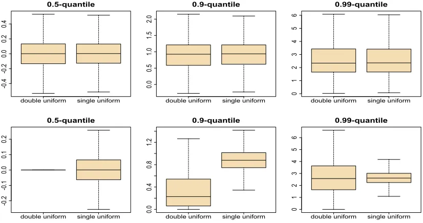
The above introduced two new parameterisations of a Gaussian mixture model, based on equation (5) and its spherical representations in Sections 2.3.1 and 2.3.2. Under the constraints imposed by the first two moment -parameters, two weakly informative priors, called the (i) single and (ii) double uniform priors, are considered below and their impact on the resulting marginal prior distributions is studied.

For the parameterisation constructed in Section 2.3.1, γ is expressed in terms of its spherical coordinates over the k−1 subset, uniformly distributed over [0, π]k−3 _×[0,2π],

and ηis associated with a uniform distribution over the_Rk_{simplex, conditional onϕ. This}

prior modelling is called the single uniform prior. Another reparametrisation is based on the spherical representations of bothγ andηleading to thedouble uniformprior, a uniform distribution on all angle parameters, $i’s andηi’s. Both priors can be argued to be weakly

informative priors, relying on uniforms for a given parameterisation.

To evaluate the difference between both modellings, using a uniform prior on ϕ2 _and

a Dirichlet distribution on the pi’s, we generated 20,000 samples from both priors. The

resulting component-wise parameter distributions are represented in Figure 1. As expected, under thesingle uniformprior, allηi’s andγi’s are uniformly distributed over thek-ball, are

-10 -5 0 5 10

0.00

0.10

0.20

0.30

log(|γ/ p|)-values

De

nsi

ty

-10 -5 0 5

0.0

0.1

0.2

0.3

0.4

log(η/ p)-values

De

nsi

ty

-20 -15 -10 -5 0 5 10

0.00

0.10

0.20

0.30

log(|γ/ p|)-values

De

nsi

ty

-20 -15 -10 -5 0 5

0.00

0.10

0.20

0.30

log(η/ p)-values

De

nsi

ty

Figure 1: Density estimate of 20,000 draws of log(|γi/

√

pi|) and log(ηi/

√

pi) from thesingle

uniform prior (red lines) and the double uniform prior (grey lines) when k = 3 (top) and k = 20 (bottom). Different grey lines indicate the density estimates fori= 1, . . . , k.

double uniform single uniform

-0 .4 -0 .2 0.0 0.2 0.4 0.5-quantile

double uniform single uniform

0.0 0.5 1.0 1.5 2.0 0.9-quantile

double uniform single uniform

0 1 2 3 4 5 6 0.99-quantile

double uniform single uniform

-0 .2 -0 .1 0.0 0.1 0.2 0.5-quantile

double uniform single uniform

0.0

0.4

0.8

1.2

0.9-quantile

double uniform single uniform

0 1 2 3 4 5 6 0.99-quantile

3

MCMC implementations

3.1

A Metropolis-within-Gibbs sampler in the Gaussian case

Given the reparameterisations introduced in Section 2, and in particular Section 2.3 for the Gaussian mixture model, different MCMC implementations are possible and we investigate in this section some of these. To this effect, we distinguish between the single and double uniform priors.

Although the target density is not too dissimilar to the target explored by early Gibbs samplers in Diebolt and Robert (1990) and Gelman and King (1990), simulating directly the new parameters implies managing constrained parameter spaces. The hierarchical na-ture of the parameterisation also leads us to consider a block Gibbs sampler that coincides with this hierarchy. Since the corresponding full conditional posteriors are not in closed form, a Metropolis-within-Gibbs sampler is implemented here with random walk proposals. In this approach, the scales of the proposal distributions are automatically calibrated to-wards optimal acceptance rates (Roberts et al., 1997; Roberts and Rosenthal, 2001, 2009). Convergence of a simulated chain is assessed based on the rudimentary convergence moni-toring technique of Gelman and Rubin (1992). The description of the algorithm is provided by a pseudo-code representation in the Supplementary Material (Figure 10). Note that the Metropolis-within-Gibbs version does not rely on latent variables and completed likelihood as in Tanner and Wong (1987) and Diebolt and Robert (1990). Following the adaptive MCMC method in Section 3 of Roberts and Rosenthal (2009), we derive the optimal scales associated with proposal densities, based on 10 batches with size 50. The scales are identified by a subscript with the corresponding parameter (see, e.g., Table 1).

For the single reparameterisation, all steps in Figure 10 are the same except that Steps 2.5 and 2.7 are ignored. When k is not large, one potential proposal density for ((ϕ2₎(t)_,(η2

1)(t), . . . ,(η2k)(t)) is a Dirichlet distribution,

((ϕ2)0,(η2₁)0, . . . ,(η_k2)0)∼Dir((ϕ2)(t−1),(η2₁)(t−1), . . . ,(η2_k)(t−1)).

Alternative proposal densities will be discussed along simulation studies in Section 4.

3.2

A Metropolis–Hastings algorithm for Poisson mixtures

Since the full conditional posteriors corresponding to the Poisson mixture (3) are not in closed form under the new parameterisation, these parameters can again be simulated by implementing a Metropolis-within-Gibbs sampler. Following an adaptive MCMC approach, the scales of the proposal distributions are automatically calibrated towards optimal accep-tance rates (Gelman et al., 1996). The description of the algorithm is provided in details by a pseudo-code in the Supplementary Material (Figure 11). Note that the Metropolis-within-Gibbs version relies on completed likelihoods.

3.3

Removing and detecting label switching

The standard parameterisation of mixture models contains weights{pi}ki=1and

per-mutations of the component indices. If an exchangeable prior is chosen on weights and component-wise parameters, which is the case for some of our priors, the posterior density is also invariant under permutations and the component-wise parameters are not identi-fiable. This phenomenon, called label switching, is well-studied in the literature (Celeux et al., 2000; Stephens, 2000b; Fr¨uhwirth-Schnatter, 2001; Jasra et al., 2005). The posterior distribution involves k! symmetric global modes and a Markov chain targetting this poste-rior is expected to explore all of them. However, MCMC chains often fail to achieve this feature (Celeux et al., 2000) and usually end up exploring one single global mode of the target.

In our reparameterisations of mixture models of Sections 2.3.1 and 2.3.2, each θi is a

function of a novel component-wise parameter from a simplex, conditional on the global parameter(s) and the weights. The mapping between both parameterisations is a one-to-one map conditional on the weights. In other words, there is a unique value for θi given

a particular set of values on this simplex and the weights. Depending on the reparam-eterisation and the choice of the prior distribution, the parameters on a simplex can be exchangeable (as, e.g., in a Poisson mixture) and with the use of a uniform prior, label switching is expected to occur. When using the double spherical representation in Section 2.3.2, the parameterisation is not exchangeable, due to the choice of the orthogonal basis. However, adopting an exchangeable prior on the weights (e.g., a Dirichlet distribution with a common parameter) and uniform priors on all angular parameters leads to an exchange-able posterior on the standard parameters of the mixture. Therefore, label switching should also occur with this prior modelling.

When an MCMC chain manages to jump between modes, the inference on each of the mixture components becomes harder (Celeux et al., 2000; Geweke, 2007). To get component-specific inference and to give a meaning to each component, various relabelling methods have been proposed in the literature (see, e.g., Fr¨uhwirth-Schnatter, 2006). A first available alternative is to reorder labels so that the mixture weights are in increasing order (Fr¨uhwirth-Schnatter, 2001). A second method proposed by, e.g., Lee et al. (2008) is that labels are reordered towards producing the shortest distance between the current posterior sample and the (or a) maximum posterior probability (MAP) estimate.

Note that the second method depends on the parameterisation of the model since both MAP and distance vary with this parameterisation. For instance, for the spherical repre-sentation of a Gaussian mixture model, the closeness of the γi’s to the MAP cannot be

determined via distance measures on $i’s, due to the symmetric features of trigonometric

functions. For such cases, we recommend to transform the MCMC sample back to the standard parameterisation, then apply a relabelling method on the standard parameters. (This step has no significant impact on the overall computing time.)

Let us denote by Sk the set of permutations on {1, . . . , k}. Then, given an MCMC

sample for the new parameters, the second relabelling technique is implemented as follows:

1. Reparameterise the MCMC sample to the standard parameterisation,{θ(t),p(t)_}T t=1.

2. Find the MAP estimate (θ∗,p∗) by computing the posterior values of the sample.

3. For eacht, reorder (θ(t),p(t)_{) as (eθ}(t)_,

e

p(t)_{) =δ}o_(θ(t)

,p(t)_{) whereδ}o _{= arg min}

δ∈Skkδ(θ

(t)

(θ∗,p∗)k.

The resulting permutation at iteration t is denoted by r(t) ∈ Sk. Label switching

occurrences in an MCMC sequence can be monitored via the changes in the sequence r(1)_{, . . . , r}(T)_{. If the MCMC chain fails to switch modes, the sequence is likely to remain at}

the same permutation. On the opposite, if a MCMC chain moves between some of the k! symmetric posterior modes, the r(t)_{’s are expected to vary.}

While the relabelling process forces one to label each posterior sample by its dis-tance from the MAP estimate, there exists an easier alternative to produce estimates for component-wise parameters. This approach is achieved byk-mean clustering on the popu-lation of all {θ(_kt),p(t)_}T

t=1. When using the Euclidean distance as in the MAP recentering,

which is the point process representation adopted in Stephens (2000a), clustering can be seen as a natural solution without the cost of relabelling an MCMC sample. When poste-rior modes are well separated, component-wise estimates from relabelling and from k-mean clustering are expected to be similar. In the event of poor switching, as exhibited for in-stance in some of our experiments, a parallel tempering resolution can be easily added to the analysis, as detailed in an earlier version of this work (Kamary et al., 2016).

4

Simulation studies for Gaussian and Poisson

mix-tures

In this section, we examine the performances of the above Metropolis-within-Gibbs method, applied to both reparameterisations defined in Section 2.3, for both simulated and real datasets.

4.1

The Gaussian case

k

= 2

In this specific case, there is no angle to consider. Two straightforward proposals are compared over simulation experiments. One is based on Beta and Dirichlet proposals:

p∗ ∼ Beta(p(t)p,(1−p(t))p), (ϕ2

∗

, η2₁∗, η₂2∗)∼ Dir(ϕ2(t), η2₁(t), η₂2(t))

(this will be called Proposal 1) and another one is based on Gaussian random walks pro-posals (Proposal 2):

log(p∗/(1−p∗))∼ N(log(p(t)/(1−p(t))), p)

(ϑ∗₁, ϑ∗₂)T ∼ N(χ(₂t), ϑI2) with

(ϕ2∗, η₁2∗, η2₂∗) = (exp(ϑ∗₁)/ϑ¯∗,exp(ϑ∗₂)/ϑ¯∗,1/ϑ¯∗), χ(₂t)= (log(ϕ2(t)/η₂2(t)),log(η₁2(t)/η2₂(t))) and ϑ¯∗ = 1 + exp(ϑ∗₁) + exp(ϑ∗₂).

The global parameters are proposed using Normal and Inverse-Gamma movesµ∗ ∼ N(¯x, µ)

respectively. We present below some analyses and also explain how MCMC methods can be used to fit mixture distributions.

Example 4.1 In this experiment, a dataset of size 50 is simulated from the mixture

0.65N(−8,2)+0.35N(−0.5,1), which implies that the true value of (ϕ2, η1, η2) is (0.813,0.149,0.406).

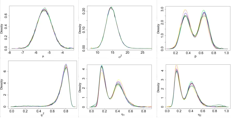
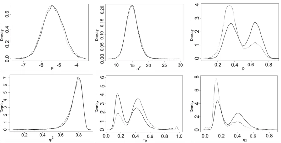
First, ten chains were simulated with Proposal 1 and different starting values. As can be seen in Figure 3, the estimated densities are almost indistinguishable among the different chains and highest-posterior regions all include the true values. The chains visited all posterior modes. The inference results about parameters using Proposals 1 and 2 are compared in Figure 4. The true values are identified by the empirical posterior distributions using both proposals. We further note that the chain derived by Proposal 1 produces more symmetric posteriors, in particular for p, ϕ, η1, η2. This suggests that the chain achieves a

better mixing behaviour.

The scales for Proposals 1 and 2 are determined by aiming at the optimal acceptance rate of Roberts et al. (1997), taken to be 0.44 for small dimensions of the parameter space. As shown in Table 1, an adaptive Metropolis-within-Gibbs strategy manages to recover acceptance rates close to optimal values. A second example in Section H, Supplementary Material, illustrates how this method using Proposal 1 behaves for a dataset with a slightly larger sample size and unlike Figure 4 the chain fails to move between posterior modes.

Figure 3: Example 4.1: Kernel estimates of the posterior densities of the parameters µ, σ, p, ϕ, ηi, based on 10 parallel MCMC chains for Proposal 1 and 2×105 iterations,

based on a single simulated sample of size 50. The true value of (µ, σ2, p, ϕ2, η1, η2) is

Figure 4: Example 4.1: Comparison between MCMC samples from our algorithm using Proposal 1 (solid line) and Proposal 2 (dashed line), with 90,000 iterations and the sample of Figure 3. The true value of (µ, σ2_{, ϕ}2_{, η}

1, η2) is (−5.375,15.747,0.813,0.149,0.406).

Proposal 1 arµ arσ arp arϕ,η µ p

0.40 0.47 0.45 0.24 0.56 77.06 99.94 Proposal 2 arµ arσ arp arϕ,η µ p ϑ

0.38 0.46 0.45 0.27 0.55 0.29 0.35

Table 1: Example 4.1: Acceptance rate (ar) and corresponding proposal scale () when the adaptive Metropolis-within-Gibbs sampler is used.

4.2

The general Gaussian mixture model

We now consider the general case of estimating a mixture for any k when the variance vector (η2

1, . . . , η2k) also has the spherical coordinate system as represented in Section 2.3.2.

All algorithms used in this section are publicly available within our R package Ultimixt. The package Ultimixt contains functions that implement adaptive determination of opti-mal scales and convergence monitoring based on Gelman and Rubin (1992) criterion. In addition, Ultimixt includes functions that summarise the simulations and compute point estimates of each parameter, such as posterior mean and median. It also produces an es-timated mixture density in numerical and graphical formats. The output further provides graphical representations of the generated parameter samples.

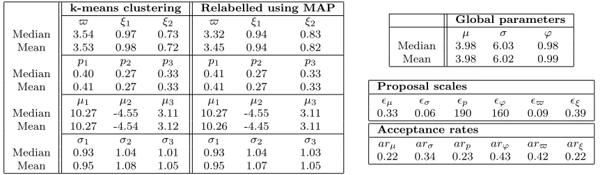
Example 4.2 The sample is made of 50 simulation from the mixture

0.27N(−4.5,1) + 0.4N(10,1) + 0.33N(3,1).

k-means clustering Relabelled using MAP

$ ξ1 ξ2 $ ξ1 ξ2

Median 3.54 0.97 0.73 3.32 0.94 0.83

Mean 3.53 0.98 0.72 3.45 0.94 0.82

p1 p2 p3 p1 p2 p3

Median 0.40 0.27 0.33 0.41 0.27 0.33

Mean 0.41 0.27 0.33 0.41 0.27 0.33

µ1 µ2 µ3 µ1 µ2 µ3

Median 10.27 -4.55 3.11 10.27 -4.55 3.11

Mean 10.27 -4.54 3.12 10.26 -4.45 3.11

σ1 σ2 σ3 σ1 σ2 σ3

Median 0.93 1.04 1.01 0.93 1.04 1.03

Mean 0.95 1.08 1.05 0.95 1.07 1.05

Global parameters

µ σ ϕ

Median 3.98 6.03 0.98

Mean 3.98 6.02 0.99

Proposal scales

µ σ p ϕ $ ξ

0.33 0.06 190 160 0.09 0.39

Acceptance rates

arµ arσ arp arϕ ar$ arξ

0.22 0.34 0.23 0.43 0.42 0.22

Table 2: Example 4.2: Point estimators of the parameters of a mixture of 3 components, proposal scales and corresponding acceptance rates.

the chain explores all posterior modes. Monitoring the chain for an angle parameter $ and pi, we illustrate the motivation of sampling η and $ through two steps in Figure 10,

Supplementary Material.

From our simulation experience of the adaptive Metropolis-within-Gibbs algorithm us-ing only a random walk proposal (restrict to Step 2.8), the simulated samples were quite close to the true values; however, the chain visited only one of the posterior modes. This lack of label switching helps us in producing point estimates directly from this MCMC out-put (Geweke, 2007) but this also shows an incomplete convergence of the MCMC sampler. To help the chain visit all posterior modes, the proposals are restricted to Step 2.4 of the Metropolis-within-Gibbs algorithm, namely using only a uniform distributionU[0,2π]. The MCMC samples on the pi’s are both well-mixed and exhibit strong exchangeability

(see Figure 12 in the Supplementary Material). However, the corresponding acceptance rate is quite low at 0.051. To increase this rate, the random walk proposal of Step 2.8 on $, namely U($(t) ₋

$, $(t) +$), is added and this clearly improves performances,

with acceptance rates all close to 0.234 and 0.44. Almost perfect label switching occurs in this case (see Figure 13 in the Supplementary Material). Hence posterior samples for η’s and $’s are generated using an independent proposal plus a random walk proposal in our adaptive Metropolis-within-Gibbs algorithm.

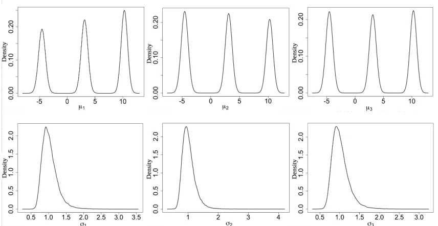
The simulated chains are almost indistinguishable component-wise, due to label switch-ing. As described in Section 3.3, we relabelled the MCMC chains using both (a) a k-means clustering algorithm and (b) a removal of label switching by permutations, as presented in Section 3.3. Point estimates of the relabelled chain are shown in Table 2 and the marginal posterior distributions of component-wise mean and standard deviation are shown in Figure 5. Bayesian estimations computed by both methods are almost identical and all parameters of the mixture distribution are accurately estimated.

Figure 5: Example 4.2: Estimated marginal posterior densities of component means and standard deviations, based on 105 MCMC iterations.

pig carcass using Gaussian mixture models and a model with six components was favoured. In this paper, a random subset of 2000 observations from the original data, made of 36326 observations, is used and estimation of the mixture model is compared to estimates based on the Gibbs sampler of bayesmby Rossi and McCulloch (2010) and on the EM algorithms ofmixtools by Benaglia et al. (2009). The data-dependent priors ofbayesmon the standard parameters are

µi ∼N(¯µ,10σi), σi2 ∼IG(ν,3) and (p1, . . . , pk)∼ Dir(α0, . . . , α0)

where IG(ν,3) is the Inverse-Gamma distribution with scale parameter 3 and degrees of freedom ν. The hyperparameters ¯µ and ν are derived from the data. Marginal prior distributions of standard parameters using either our double uniform prior (Section 2.3.2) or priors obtained by bayesm are compared graphically in Figure 7. While the priors for µi and σi yielded by bayesm do not vary withk, our marginal posteriors get more skewed

toward 0 with k but has a longer tail to provide flexible supports for component-wise location and scale parameters. We stress that we fixed the global mean and variance to 0 and 1 here, implying that the outcome will be more variable when the Jeffrey prior is called.

(a (b

(c (d

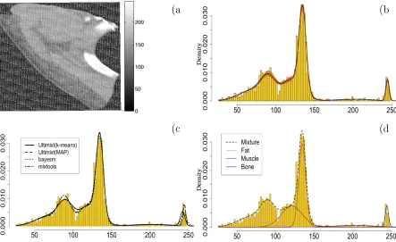
Figure 6: CT image data and the analysis result: (a) The CT image of a cross-section from a pork carcass in grey-scale units. The right bar describes the grey-scale, 0-256. (b) Representation of last 500 MCMC iterations as mixture densities with the overlaid average curve for k = 6 components (dark line) (c) Comparison between the mixture density estimates obtained byUltimixt,mixtoolsandbayesm(d) Mixture model overlapping with distributions of each components: Two violet, brown and blue lines are distributions representing fat tissue, muscle and bone, respectively.

estimates. As can be seen from Figure 6 (with exact values in Table 3 from the Supple-mentary Material), the estimates from the three packages Ultimixt, mixtools and bayesm

are relatively similar and tissue composition similar to the findings of McGrory (2013) is observed. Figure 6 (d) shows how the composition of tissues is modelled by six Gaussian components which can be interpreted as follows: two components correspond to fat (33%), two to muscle (59%), one to bone (4%) and the remaining component models the mixed tissue of muscle and bone (4%). Among the six components, the biggest component has the weight of 34% and corresponds to muscle. In the intended application, this is the quantity of interest: the higher this percentage, the higher the meat quality of the animal.

4.3

Poisson mixtures

The following example demonstrates how a weakly informative prior for a Poisson mixture is associated with a MCMC algorithm. Under the constraint, Pk

i=1γi = 1, the Dirichlet

prior with the common parameter is used on local parameters γi. Any other vague proper

-10 -5 0 5 10 0.0 0.2 0.4 0.6 0.8 1.0 µ-values De nsi ty

0 2 4 6 8

0.0 1.0 2.0 3.0 σ-values De nsi ty

0.0 0.4 0.8

0 1 2 3 4 p-values De nsi ty

-10 -5 0 5 10

0.0 0.5 1.0 1.5 2.0 2.5 µ-values De nsi ty

0 2 4 6 8

0 1 2 3 4 σ-values De nsi ty

0.0 0.4 0.8

0 1 2 3 4 5 6 p-values De nsi ty

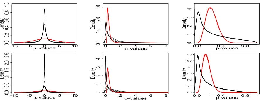
Figure 7: CT image data : Density estimate of 20,000 draws ofµi, σiandpi (i= 1, . . . , k)

from the prior by bayesm(red lines)and our double uniform prior (black lines)assuming a global mean of 0 and variance of 1 when k = 4 (first row)and k= 6 (second row). For the prior by bayesmhyperparameters α0 = 5, ¯µ= 0 andν = 3 are obtained usingbayesm.

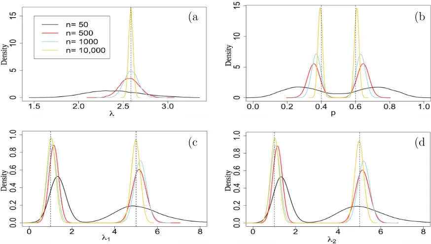
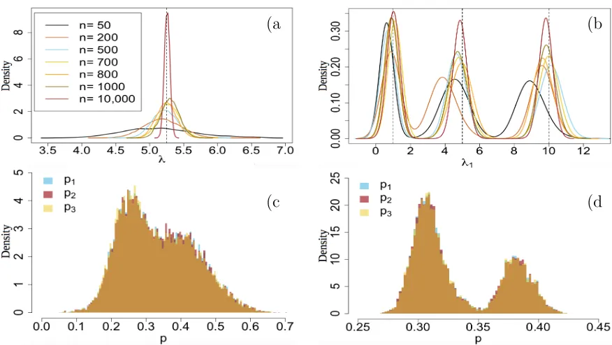
Example 4.4 The following two Poisson mixture models are considered for various sample sizes, from 50 to 104_.

Model 1: 0.6P(1) + 0.4P(5)

Model 2: 0.3P(1) + 0.4P(5) + 0.3P(10)

Figures 8 and 9 display the performances of the Metropolis-within-Gibbs sampler (see also Figure 11 in Supplementary Material). The convergence of the resulting sequence of estimates to the true values is illustrated by the figures as the number of data points increases. While label switching occurs with our prior modelling, as shown in both Figures 8 and 9, the point estimate of each parameter subjected to label switching (component weights and means) can be computed by relabelling the MCMC draws. We then derive point estimates by clustering over the parameter space, using k-mean clustering, resulting in close agreement with the true values.

5

Conclusion

(a (b

(c (d

Figure 8: Mixture of two Poisson distributions 4.4: Comparison between the empiri-cal densities of 5 104 _{MCMC simulations of (a) the global mean, (b) the weight and (c)-(d)}

component means. True values are indicated by dashed lines. The different colors in all graphs correspond to the different sample sizes indicated in (a).

Gaussian, Poisson and exponential distributions and their compound extensions. While the notion of a non-informative or objective prior is mostly open to interpretations and somehow controversial, we argue we have defined in this paper what can be considered as the first reference prior for mixture models. We have shown further that relatively standard simulation algorithms are able to handle these new parametrisations, as exhibited by our Ultimixt R package, and that they can manage the computing issues connected with label switching.

While the extension to non-Gaussian cases with location-scale features is shown here to be conceptually straightforward, considering this reparameterisation in higher dimensions is delicate when made in terms of the covariance matrices. Indeed, even though we can easily set the variance matrix of the mixture model as a reference parameter, reparameterising the component variance matrices against this reference matrix and devising manageable priors remains an open problem that we are currently exploring.

References

Andrews, D. F.and Mallows, C. L.(1974). Scale mixtures of normal distributions. J. Royal Statist.

Society Series B,3699–102.

Benaglia, T., Chauveau, D., Hunter, D. and Young, D. (2009). mixtools: An R package for

(a (b

(c (d

Figure 9: Mixture of three Poisson distributions: Comparison between the empirical densities of 5 104 _{MCMC simulations of (a) the global mean, (b) the component mean λ}

1

and weights for two samples of size (c) n= 200 and (d) n= 104_{. True values are indicated}

by dashed lines. The different colors in all graphs correspond to the different sample sizes indicated in (a). total number of MCMC iterations is 5 104 _{with a burn-in of 10}3 _iterations.

Berkhof, J., van Mechelen, I. and Gelman, A. (2003). A Bayesian approach to the selection and testing of mixture models. Statistica Sinica,13423–442.

Berger, J.(2004). The case for objective Bayesian analysis. Bayesian Analysis,11–17.

Berger, J., Bernardo, J. and Sun, D. (2009). Natural induction: An objective Bayesian approach.

Rev. R. Acad. Cien. Serie A. Mat.,103125–135.

Bernardo, J. and Gir`on, F. (1988). A Bayesian analysis of simple mixture problems. In Bayesian

Statistics 3 (J. Bernardo, M. DeGroot, D. Lindley and A. Smith, eds.). Oxford University Press, Oxford, 67–78.

Celeux, G.,Hurn, M. andRobert, C.(2000). Computational and inferential difficulties with mixture posterior distributions. J. Amer. Statist. Assoc.,95(3)957–979.

Chib, S. (1995). Marginal likelihood from the Gibbs output. J. Amer. Statist. Assoc.,901313–1321.

Diebolt, J. and Robert, C. (1990). Estimation des param`etres d’un m´elange par ´echantillonnage bay´esien. Notes aux Comptes–Rendus de l’Acad´emie des Sciences I,311653–658.

Diebolt, J.andRobert, C.(1994). Estimation of finite mixture distributions by Bayesian sampling. J.

Royal Statist. Society Series B, 56363–375.

Feller, W. (1971). An Introduction to Probability Theory and its Applications, vol. 2. John Wiley, New York.

Figueiredo, M.andJain, A.(2002). Unsupervised learning of finite mixture models. Pattern Analysis

and Machine Intelligence, IEEE Transactions,24381–396.

Fr¨uhwirth-Schnatter, S. (2001). Markov chain Monte Carlo estimation of classical and dynamic switching and mixture models. J. Amer. Statist. Assoc.,96 194–209.

Fr¨uhwirth-Schnatter, S.(2006). Finite Mixture and Markov Switching Models. Springer-Verlag, New York, New York.

Gelman, A., Gilks, W. and Roberts, G. (1996). Efficient Metropolis jumping rules. In Bayesian

Statistics 5 (J. Berger, J. Bernardo, A. Dawid, D. Lindley and A. Smith, eds.). Oxford University Press, Oxford, 599–608.

Gelman, A. and King, G. (1990). Estimating the electoral consequences of legislative redistricting. J. Amer. Statist. Assoc.,85274–282.

Gelman, A. andRubin, D. (1992). Inference from iterative simulation using multiple sequences (with discussion). Statist. Science 457–472.

Geweke, J. (2007). Interpretation and inference in mixture models: Simple MCMC works.

Com-put. Statist. Data Analysis, 513529–3550.

Gleser, L. (1989). The Gamma distribution as a mixture of exponential distributions. Amer. Statist., 43115–117.

Gleser, M., Carlin, B. P.andSrivastiva, M. S.(1995). Probability matching priors for linear cali-bration. TEST,4333–357.

Grazian, C.andRobert, C.(2015). Jeffreys priors for mixture estimation. In Bayesian Statistics from

Methods to Models and Applications (S. Fr¨uhwirth-Schnatter, A. Bitto, G. Kastner and A. Posekany, eds.). Springer Proceedings in Mathematics & Statistics, vol 126, Springer, 37–48.

Griffin, J. E.(2010). Default priors for density estimation with mixture models. Bayesian Analysis, 5 45–64.

Jasra, A., Holmes, C. andStephens, D. (2005). Markov Chain Monte Carlo methods and the label switching problem in Bayesian mixture modeling. Statist. Sci.,20 50–67.

Jeffreys, H.(1939). Theory of Probability. 1st ed. The Clarendon Press, Oxford.

Kamary, K.andLee, K.(2017). Ultimixt: Bayesian Analysis of a Non-Informative Parametrisation for Gaussian Mixture Distributions. R package version 2.0,

Kamary, K., Lee, K.and Robert, C. (2016). Non-informative reparameterisations for location-scale mixtures. ArXiv e-prints. 1601.01178.

Kamary, K.,Mengersen, K.,Robert, C.andRousseau, J.(2014). Testing hypotheses as a mixture estimation model. ArXiv e-prints. 1412.4436.

Kass, R.andWasserman, L.(1996). Formal rules of selecting prior distributions: a review and annotated bibliography. J. Amer. Statist. Assoc.,91343–1370.

Lee, J., (2009). Bayesian hybrid algorithms and models : implementation and associated issues PhD thesis. Queensland University of Technology.

Lee, K., Marin, J.-M., Mengersen, K. and Robert, C. (2009). Bayesian inference on mixtures of distributions. In Perspectives in Mathematical Sciences I: Probability and Statistics (N. N. Sastry, M. Delampady and B. Rajeev, eds.). World Scientific, Singapore, 165–202.

Lee, K.,Marin, J.-M.,Mengersen, K. L.andRobert, C.(2008). Bayesian inference on mixtures of distributions. InPlatinum Jubilee of the Indian Statistical Institute(N. N. Sastry, ed.). Indian Statistical Institute, Bangalore.

Marin, J.-M.,Mengersen, K. andRobert, C.(2005). Bayesian modelling and inference on mixtures of distributions. In Handbook of Statistics (C. Rao and D. Dey, eds.), vol. 25. Springer-Verlag, New York, 459–507.

McGrory, C.A.(2013). Variational Bayesian inference for mixture models . InCase studies in Bayesian

statistical modelling and analysis (C. L. Alston, K. L. Mengersen, A. N. Pettitt, eds.) John Wiley & Sons , 388–402.

Mengersen, K. and Robert, C. (1996). Testing for mixtures: A Bayesian entropic approach (with discussion). InBayesian Statistics 5 (J. Berger, J. Bernardo, A. Dawid, D. Lindley and A. Smith, eds.). Oxford University Press, Oxford, 255–276.

Neal, R.(1999). Erroneous results in “Marginal likelihood from the Gibbs output“. Tech. rep., University of Toronto. URL_{http://www.cs.utoronto.ca/~radford}.

O’Hagan, A.(1994). Bayesian Inference. No. 2B in Kendall’s Advanced Theory of Statistics, Chapman and Hall, New York.

Richardson, S. andGreen, P. (1997). On Bayesian analysis of mixtures with an unknown number of components (with discussion). J. Royal Statist. Society Series B,59731–792.

Rissanen, J.(2012). Optimal Estimation of Parameters. Cambridge University Press.

Robert, C. and Titterington, M. (1998). Reparameterisation strategies for hidden Markov models and Bayesian approaches to maximum likelihood estimation. Statistics and Computing,8145–158.

Roberts, G. O., Gelman, A. and Gilks, W. R. (1997). Weak convergence and optimal scaling of random walk Metropolis algorithms. The Annals of Applied probability,7110–120.

Roberts, G. O. and Rosenthal, S. J. (2001). Optimal scaling for various Metropolis-Hastings algo-rithms. Statist. Science,16351–367.

Roberts, G. O. and Rosenthal, S. J. (2009). Examples of adaptive MCMC. J. Computational and

Graphical Statist.,18349 –367.

Roeder, K. (1990). Density estimation with confidence sets exemplified by superclusters and voids in galaxies. J. Amer. Statist. Assoc.,85617–624.

Rossi, P. and McCulloch, R.(2010). Bayesm: Bayesian inference for marketing/micro-econometrics.

R package version, 3.0-2.

Rousseau, J. and Mengersen, K. (2011b). Asymptotic behaviour of the posterior distribution in overfitted mixture models. J. Royal Statist. Society Series B,73 689–710.

Rubio, F.andSteel, M.(2014). nference in two-piece location-scale models with Jeffreys priors.Bayesian

Stephens, M.(2000a). Bayesian analysis of mixture models with an unknown number of components—an alternative to reversible jump methods. Ann. Statist.,2840–74.

Stephens, M. (2000b). Dealing with label switching in mixture models. J. Royal Statist. Society Series B,62(4) 795–809.

Tanner, M.andWong, W.(1987). The calculation of posterior distributions by data augmentation. J.

Amer. Statist. Assoc.,82528–550.

Thompson, J. andKinghorn, B. (1992). CATMAN-A program to measure CAT-Scans for prediction of body components in live animals. Proceeding of the Australian Association of Animal Breeding and Genetics.(AAAGB Distribution Service, The University of New England: Armidale, NSW),10560-564.

Wasserman, L. (1999). Asymptotic inference for mixture models by using data-dependent priors. J.

Royal Statist. Society Series B, 61159–180.

Welch, B. and Peers, H. (1963). On formulae for confidence points based on integrals of weighted likelihoods. J. Royal Statist. Society Series B,25318–329.

Supplementary material

A

Proof of Lemma 1

The population mean is given by

Eθ,p[X] =

k

X

i=1

piEf(·|θi)[X] =

k

X

i=1

piµi

where _Ef(·|θi)[X] is the expected value component i. Similarly, the population variance is

given by

varθ,p(X) =

k

X

i=1

piEf(·|θi)[X

2_]−

Eθ,p[X]2 =

k

X

i=1

pi(σ2i +µ

2

i)−Eθ,p[X]2,

which concludes the proof.

B

Proof of Lemma 2

The result is a trivial consequence of Lemma 1. The population mean is

Eθ,p[X] =

k

X

i=1

piµi = k

X

i=1

pi(µ+σαi) =µ+σ k

X

i=1

and the first constraint follows. The population variance is

varθ,p(X) =

k

X

i=1

piσi2+ k

X

i=1

pi(µ2i −Eθ,p[X]2)

=

k

X

i=1

piσ2τi2+ k

X

i=1

pi(µ2+ 2σµαi+σ2α2i −µ

2₎

=

k

X

i=1

piσ2τi2+ k

X

i=1

piσ2α2i

The last equation simplifies to the second constraint above.

C

Proof of Theorem 1

When n = 1, it is easy to show that the posterior is not proper. The marginal likelihood is then

Mk(x1) =

k

X

i=1

Z

pif(x1|µ+σαi, σ2τi2)π(µ, σ,p,α,τ) d(µ, σ,p,α,τ)

=

k

X

i=1

Z Z _p

i

√

2πσ2_τ

i

exp ₋

(x1−µ−σαi)2

2τ2

iσ2

d(µ, σ)

π(p,α,τ) d(p,α,τ)

=

k

X

i=1

Z Z ∞

0

pi

σ dσ

π(p,α,τ) d(p,α,τ)

The integral against σ is then not defined.

For two data-points,x1, x2 ∼Pk_i=1pif(µ+σαi, σ2τi2), the associated marginal likelihood

is

Mk(x1, x2) =

Z 2 Y j=1 ( _k X i=1

pif(xj|µ+σαi, σ2τi2)

)

π(µ, σ,p,α,τ) d(µ, σ,p,α,τ)

= k X i=1 k X j=1 Z

pipjf(x1|µ+σαi, σ2τi2)f(x2|µ+σαj, σ2τj2)π(µ, σ,p,α,τ) d(µ, σ,p,α,τ) .

If all thosek2integrals are proper, the posterior distribution is proper. An arbitrary integral (1≤i, j ≤k) in this sum leads to

Z

pipjf(x1|µ+σαi, σ2τi2)f(x2|µ+σαj, σ2τj2)π(µ, σ,p,α,τ) d(µ, σ,p,α,τ)

=

Z (Z _p

ipj

2πσ3_τ

iτj

exp "

−(x1−µ−σαi)2

2τ2

iσ2

+ −(x2−µ−σαj)

2

2τ2

jσ2

#

d(µ, σ) )

π(p,α,τ) d(p,α,τ)

=

Z (Z ∞

0

pipj

√

2πσ2q_τ2

i +τj2

exp "

−1 2(τ2

i +τj2)

1

σ2(x1−x2)

2₊ 2

σ(x1−x2)(αi−αj)

+(αi−αj)2

!# dσ

)

Substituting σ= 1/z, the above is integrated with respect to z, leading to

Z (Z ∞

0

pipj

√

2πqτ2

i +τj2

exp −1

2(τ2

i +τj2)

z2(x1−x2)2 + 2z(x1−x2)(αi−αj)

+(αi−αj)2

!! dz

)

π(p,α,τ) d(p,α,τ)

=

Z (Z ∞

0

pipj

√

2πqτ2

i +τj2

exp −(x1−x2)

2

2(τ2

i +τj2)

z+ αi−αj x1−x2

2 !

dz )

π(p,α,τ) d(p,α,τ)

= Z

pipj

|x1−x2|

Φ 

−

αi−αj

x1−x2

|x1−x2|

q τ2

i +τj2



π(p,α,τ) d(p,α,τ),

where Φ is the cumulative distribution function of the standardised Normal distribution. Given that the prior is proper on all remaining parameters of the mixture, it follows that the integrand is bounded by 1/|x1−x2|, and so it integrates against the remaining components

of θ. Now, consider the case n≥3. Since the posterior π(θ|x1, x2) is proper, it constitutes

a proper prior when considering only the observations x3, . . . , xn. Therefore, the posterior

is almost everywhere proper.

D

Proof of Theorem 2

Considering one single positive observation x1, the marginal likelihood is

Mk(x1) =

k

X

i=1

Z

pif(x1|λγi/pi)π(λ, γγγ, ppp)d(λ, γγγ, ppp)

=

k

X

i=1

Z Z ∞

0

piexp(−λγi/pi)(λγi/pi)x1/x1!π(λ)dλ

π(γγγ, ppp)d(γγγ, ppp)

=

k

X

i=1

Z

pi(γi/pi)x1/x1!

Z ∞

0

exp(−λγi/pi)λx1−1dλ

π(γγγ, ppp)d(γγγ, ppp)

=

k

X

i=1

Z

(pi/x1)π(γγγ, ppp)d(γγγ, ppp)

Since the prior is proper on all remaining parameters of the mixture, the integrals in the above sum are all finite. The posterior π(λ, γγγ, ppp|x1) is therefore proper and it constitutes

a proper prior when considering further observations x2, . . . , xn. Therefore, the resulting

E

Proof of Theorem 3

Considering one single observation x1, the marginal likelihood is

Mk(x1) =

k

X

i=1

Z

pif(x1|pi/λγi)π(λ, γγγ, ppp)d(λ, γγγ, ppp)

=

k

X

i=1

Z Z ∞

0

piexp(−pix/λγi)pi/λγiπ(λ)dλ

π(γγγ, ppp)d(γγγ, ppp)

=

k

X

i=1

Z pi

Z ∞

0

pi/_λγiexp(−λγ_ix₁/p_i)dλπ(γγγ, ppp)d(γγγ, ppp)

=

k

X

i=1

Z

(pi/x1)π(γγγ, ppp)d(γγγ, ppp).

Since the prior is proper on all remaining parameters of the mixture, the integrals in the above sum are all finite. The posterior π(λ, γγγ, ppp|x1) is therefore proper and it constitutes

a proper prior when considering further observations x2, . . . , xn. Therefore, the resulting

F

Pseudo-code representations of the MCMC

algo-rithms for the Normal and Poisson cases

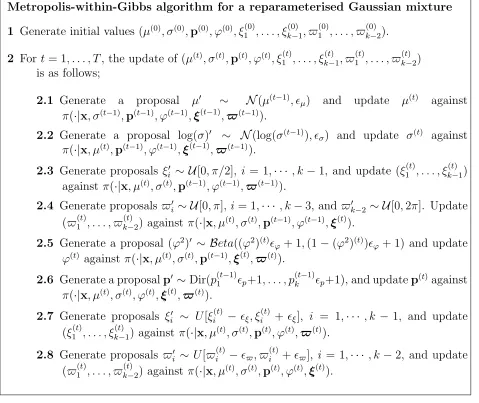
Metropolis-within-Gibbs algorithm for a reparameterised Gaussian mixture

1 Generate initial values (µ(0)_{, σ}(0)_,p(0)_{, ϕ}(0)_{, ξ}(0) 1 , . . . , ξ

(0)

k−1, $ (0)

1 , . . . , $ (0)

k−2).

2 For t= 1, . . . , T, the update of (µ(t), σ(t),p(t), ϕ(t), ξ₁(t), . . . , ξ_k(t₋)₁, $₁(t), . . . , $(_kt₋)₂) is as follows;

2.1 Generate a proposal µ0 ∼ N(µ(t−1), µ) and update µ(t) against

π(·|x, σ(t−1),p(t−1), ϕ(t−1),ξ(t−1),$(t−1)).

2.2 Generate a proposal log(σ)0 ∼ N(log(σ(t−1)_),

σ) and update σ(t) against

π(·|x, µ(t),p(t−1), ϕ(t−1),ξ(t−1),$(t−1)).

2.3 Generate proposals ξ_i0 ∼ U[0, π/2], i = 1,· · · , k−1, and update (ξ₁(t), . . . , ξ_k(t₋)₁) againstπ(·|x, µ(t)_{, σ}(t)_,p(t−1)_{, ϕ}(t−1)_,$(t−1)_).

2.4 Generate proposals$0_i ∼ U[0, π],i= 1,· · · , k−3, and $_k0₋₂ ∼ U[0,2π]. Update ($₁(t), . . . , $_k(t₋)₂) against π(·|x, µ(t)_{, σ}(t)_,p(t−1)_{, ϕ}(t−1)_,ξ(t)

).

2.5 Generate a proposal (ϕ2)0 ∼ Beta((ϕ2)(t)ϕ + 1,(1−(ϕ2)(t))ϕ + 1) and update

ϕ(t) _{against π(·|x, µ}(t)_{, σ}(t)_,p(t−1)_,ξ(t)

,$(t)_).

2.6 Generate a proposalp0 ∼Dir(p(₁t−1)p+1, . . . , p

(t−1)

k p+1), and updatep

(t)_against

π(·|x, µ(t), σ(t), ϕ(t),ξ(t),$(t)).

2.7 Generate proposals ξ_i0 ∼ U[ξ(_it) − ξ, ξ

(t)

i + ξ], i = 1,· · · , k −1, and update

(ξ₁(t), . . . , ξ_k(t₋)₁) against π(·|x, µ(t)_{, σ}(t)_,p(t)_{, ϕ}(t)_,$(t)_).

2.8 Generate proposals $0_i ∼ U[$(_it)−$, $

(t)

i +$], i = 1,· · · , k−2, and update

($₁(t), . . . , $_k(t₋)₂) against π(·|x, µ(t)_{, σ}(t)_,p(t)_{, ϕ}(t)_,ξ(t)_).

Figure 10: Pseudo-code representation of the Metropolis-within-Gibbs algorithm used in this paper for reparameterisation (ii) of the Gaussian mixture model, based on two sets of spherical coordinates. For simplicity’s sake, we denote p(t) _{= (p}(t)

1 , . . . , p

(t)

k ), x =

(x1, . . . , xn), ξ(t)= (ξ

(t)

1 , . . . , ξ

(t)

k−1) and $

(t) _{= ($}(t)

1 , . . . , $

(t)

Metropolis-within-Gibbs algorithm for a reparameterised Poisson mixture

1 Generate initial values (λ(0)_{, γγγ}(0)_,p(0)_).

2 For t= 1, . . . , T, the update of (λ(t), γγγ(t),p(t)) is as follows;

2.1 Generate a proposal λ0 ∼ N(log(X), λ) and update λ(t) against

π(·|x, γγγ(t−1)_,p(t−1)_).

2.2 Generate a proposal γγγ0 ∼ Dir(γ₁(t−1)γ + 1, . . . , γ(t

−1)

k γ + 1), and update γγγ

(t)

againstπ(·|x, λ(t)_,p(t−1)_).

2.3 Generate a proposal p0 ∼ Dir(p₁(t−1)p + 1, . . . ,p

(t−1)

k p + 1), and update p(t)

againstπ(·|x, λ(t), γγγ(t)).

Figure 11: Pseudo-code representation of the Metropolis-within-Gibbs algorithm used to approximate the posterior distribution of the reparameterisation of the Poisson mixture. For i= 1, . . . , k, we denoteγγγ = (γ1, . . . , γk), p(t) = (p

(t)

1 , . . . , p

(t)

k ) and x= (x1, . . . , xn). X

G

Convergence graphs for Example 4.2

Figure 12: Example 4.2: (Left) Evolution of the sequence ($(t)) and (Right) histograms of the simulated weights based on 105 _{iterations of an adaptive Metropolis-within-Gibbs}

algorithm with independent proposal on $.

Figure 13: Example 4.2: Traces of 105 _{simulations from the posterior distributions of the}

component means, standard deviations and weights, involving an additional random walk proposal on $.

H

An illustration of the proposal impact on Old

Faith-ful

We analysed the R benchmark Old Faithful dataset, using the 272 observations of eruption times and a mixture model with two components. The empirical mean and variance of the observations are (3.49,1.30).

When using Proposal 1, the optimal scalesµ, p, after 50,000 iterations are 0.07,501.1,

Figure 14: Old Faithful dataset: Posterior distributions of the parameters of a two-component mixture distribution based on 50,000 MCMC iterations.

I

Values of estimates of the mixture parameters

be-hind the CT dataset

k-means clustering (Ultimixt)

p1 p2 p3 p4 p5 p6

Median 0.16 0.17 0.25 0.34 0.04 0.04

Mean 0.16 0.17 0.25 0.34 0.03 0.04

µ1 µ2 µ3 µ4 µ5 µ6

Median 68.75 89.88 121.0 134.6 201.3 244.4

Mean 68.68 89.88 121.1 134.6 203.3 242.2

σ1 σ2 σ3 σ4 σ5 σ6

Median 17.37 9.380 13.66 4.613 23.62 2.055

Mean 17.38 9.388 13.69 4.615 22.72 2.995

Relabelled using MAP (Ultimixt)

p1 p2 p3 p4 p5 p6

Median 0.16 0.17 0.25 0.34 0.03 0.04

Mean 0.16 0.17 0.25 0.34 0.03 0.04

2.5% 0.15 0.16 0.24 0.33 0.03 0.04

97.5% 0.17 0.18 0.27 0.36 0.04 0.05

µ1 µ2 µ3 µ4 µ5 µ6

Median 68.71 89.91 121.0 134.6 201.0 244.4

Mean 68.67 89.92 121.1 134.6 201.1 244.3

2.5% 65.89 88.85 120.4 134.2 196.3 243.9

97.5% 71.10 90.82 122.5 135.1 206.3 244.9

σ1 σ2 σ3 σ4 σ5 σ6

Median 17.37 9.386 13.62 4.615 23.62 2.054

Mean 17.38 9.391 13.71 4.621 23.66 2.047

2.5% 16.43 8.673 12.83 4.370 21.89 1.822

97.5% 18.38 10.12 14.80 4.871 25.67 2.220

Gibbs sampler (bayesm)

p1 p2 p3 p4 p5 p6

Mean 0.17 0.18 0.21 0.36 0.04 0.04

µ1 µ2 µ3 µ4 µ5 µ6

Mean 69.74 88.99 119.94 134.48 196.69 243.94

σ1 σ2 σ3 σ4 σ5 σ6

Mean 18.44 8.048 10.85 4.956 24.08 3.808

EM estimate (mixtools)

p1 p2 p3 p4 p5 p6

0.15 0.18 0.27 0.33 0.04 0.04

µ1 µ2 µ3 µ4 µ5 µ6

67.62 88.57 121.9 134.6 203.2 244.5

σ1 σ2 σ3 σ4 σ5 σ6

17.42 7.818 13.84 4.579 23.27 1.841

J

R codes