A log linear time algorithm for constrained changepoint detection

(1)

A log-linear time algorithm for constrained changepoint detection

Toby Dylan Hocking ([email protected])

Guillem Rigaill ([email protected])

Paul Fearnhead ([email protected])

Guillaume Bourque ([email protected])

March 10, 2017

Abstract

Changepoint detection is a central problem in time series and genomic data. For some applications, it is natural to impose constraints on the directions of changes. One example is ChIP-seq data, for which adding an up-down constraint improves peak detection accuracy, but makes the optimization problem more complicated. We show how a recently proposed functional pruning technique can be adapted to solve such constrained changepoint detection problems. This leads to a new algorithm which can solve problems with arbitrary affine constraints on adjacent segment means, and which has empirical time complexity that is log-linear in the amount of data. This algorithm achieves state-of-the-art accuracy in a benchmark of several genomic data sets, and is orders of magnitude faster than existing algorithms that have similar accuracy. Our implementation is available as the PeakSegPDPA function in the coseg R package,https://github.com/tdhock/coseg

(2)

1 Introduction

Changepoint detection is a central problem in fields such as finance or genomics, wherendata are gathered in a se-quence over time or space. Many models define the optimal changepoints using maximum likelihood, resulting in a discrete optimization problem. Multiple changepoint detection models seek the optimalKsegments (K−1changes), which amounts to optimizing likelihood parameters over a space that containsO(nK−1)discrete arrangements of changepoints. In general this problem can be solved inO(Kn2)time using the original dynamic programming al-gorithm of Auger and Lawrence [1989]. Recently proposed pruning techniques reduce the number of changepoints considered by the algorithm, thus reducing time complexity toO(Knlogn)while maintaining optimality [Rigaill, 2010, Johnson, 2013, Maidstone et al., 2016].

In “unconstrained” changepoint models, there are no contraints between model parameters on separate segments. To regularize and obtain a more interpretable model, it is often desirable to introduce constraints between model parameters before and after changepoints. For example, the main problem that motivates this paper is peak detection in ChIP-seq data, which provide noisy measurements of protein binding or modification throughout a genome [Bailey et al., 2013]. An up-down constrained changepoint detection model has been shown to achieve state-of-the-art peak detection accuracy in ChIP-seq data [Hocking et al., 2015]. The constraints of this model force an up change in the segment mean parameter after each down change, and vice versa. The fastest existing solver for this problem is the Constrained Dynamic Programming Algorithm (CDPA), which has two issues. First, it is a heuristic algorithm that is not guaranteed to recover the optimal solution. Second, itsO(Kn2₎_{quadratic time complexity is too slow for use on} large data sets. In this paper we propose a new algorithm that fixes both of these issues.

1.1 Contributions and organization

We begin by discussing previous research into pruning techniques for solving unconstrained changepoint detection problems (Section 2), then state the constrained optimization problems (Section 3). Our main contribution is Sec-tion 4, which generalizes the funcSec-tional pruning technique of Rigaill [2010], thus providing a new Generalized Pruned Dynamic Progamming Algorithm (GPDPA) for solving a class of constrained changepoint detection problems. We show that the GPDPA achieves state-of-the-art speed and accuracy in genomic data with several different labeled patterns (Section 5), then conclude by discussing the significance of our contributions (Section 6).

2 Related work

There are many efficient algorithms available for computing the optimalK−1changepoints inndata points. Auger and Lawrence [1989] proposed anO(Kn2₎_{algorithm for computing the sequence of models with}₁_{, . . . , K}_segments. Jackson et al. [2005] consider a related approach, which introduces a penalty for each changepoint, rather than fixing the number of changepoints. TheirO(n2₎_{algorithm computes the single model for a given penalty constant}_λ_{. Both of} these algorithms recover the optimal solution, and follow from using dynamic programming updates [Bellman, 1961] to recursively compute the maximum likelihood from 1 tondata points. Alternatively there are methods which are

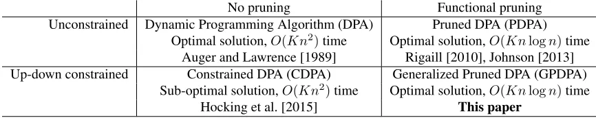
No pruning Functional pruning

Unconstrained Dynamic Programming Algorithm (DPA) Pruned DPA (PDPA) Optimal solution,O(Kn2₎_time _{Optimal solution,}_O₍_Kn_log_n₎_time

Auger and Lawrence [1989] Rigaill [2010], Johnson [2013]

Up-down constrained Constrained DPA (CDPA) Generalized Pruned DPA (GPDPA)

Sub-optimal solution,O(Kn2₎_time _{Optimal solution,}_O₍_Kn_log_n₎_time

[image:3.612.88.521.552.638.2]

Hocking et al. [2015] This paper

Table 1: Our contribution is the Generalized Pruned Dynamic Programming Algorithm (GPDPA), which uses a functional pruning technique to compute the constrained optimal K−1 changepoints in a sequence ofndata, in

(4)

computationally faster but are not guaranteed to find the optimal segmentation. The most popular of these is the binary segmentation algorithm which hasO(Kn)worst-case time complexity [Scott and Knott, 1974]. An L1 relaxation of this problem is known as the fused lasso signal approximator, for which efficient solvers also exist [Hoefling, 2010].

Several pruning methods have been recently proposed in order to reduce time complexity, while maintaining optimality. Rigaill [2010] and Johnson [2011] independently discovered a functional pruning technique, which results in algorithms withO(nlogn)average time complexity. Killick et al. [2011] proposed an inequality pruning technique, which results in an algorithm with average time complexity fromO(n)toO(n2_{), depending on the number of changes.} Maidstone et al. [2016] provides a clear discussion on the differences between the two pruning techniques.

All algorithms discussed thus far are for solving problems with no constraints between adjacent segment mean pa-rameters, but there are many examples of constrained changepoint detection models. Rather than searching all possible changepoints and likelihood parameters, the idea is to use a constraint in order to search a smaller, more interpretable model space. For example, Haiminen et al. [2008] propose anO(Kn2₎_{algorithm for unimodal regression, which} enforces no up changes after the first down change. Hocking et al. [2015] proposed anO(Kn2)algorithm for peak detection, which enforces a down change after each up change, and vice versa.

Isotonic regression is another example of a constrained changepoint detection model. There is no limit on the number of segmentsK, but the segment means are constrained to be non-decreasing. This problem can be solved inO(n)time using the pool-adjacent-violators algorithm [Mair et al., 2009], or inO(nlogn)time using a dynamic programming algorithm [Rote, unpublished]. An L1 relaxation of this problem is known as nearly-isotonic regression [Tibshirani et al., 2011]. A problem known as reduced isotonic regression occurs by imposing an additional constraint ofKsegments [Schell and Singh, 1997]. The techniques for solving this problem lead to sub-quadratic time algorithms [Hardwick and Stout, 2014], but do not generalize to other kinds of constraints (such as unimodal regression or peak detection).

Our contribution in this paper is proving that the functional pruning technique can be generalized to constrained changepoint models (Table 1). Our resulting Generalized Pruned Dynamic Programming Algorithm (GPDPA) enjoys

O(Knlogn)time complexity, and works for any changepoint model with affine constraints between adjacent segment means (including isotonic regression, unimodal regression, and peak detection).

3 Isotonic regression and changepoint models

Although our proposed algorithm can solve many constrained changepoint detection problems (Section 4.5), we will simplify our discussion by emphasizing the isotonic regression model.

3.1 Classical isotonic regression

The classical isotonic regression model is defined as the most likely sequence of non-decreasing segment means. More precisely, assume that the datay∈Rnare a realization of a probability distribution with mean parameterm∈Rn. For

example, assumingyt∼ N(mt, σ2)and performing maximum likelihood inference results in a convex minimization

problem with affine constraints,

minimize m∈Rn

n

X

t=1

`(yt, mt) (1)

subject to mt≤mt+1,∀t < n.

The convex loss function`:_R×_R→_Rin the case of the Gaussian likelihood is the square loss`(y, m) = (y−m)2_. This optimization problem (1) is referred to as isotonic regression, and can be efficiently solved inO(n)time using the Pool-Adjacent-Violators Algorithm (PAVA) [Best and Chakravarti, 1990].

Since isotonic regression imposes no limit on the number of changepoints (mt < mt+1), it tends to overfit. For example, consider the toy data sety =

2 5 30 34 600 621

∈ R6. Because these data are strictly

increasing, the isotonic regression (1) solution is the trivial modelmt =yt. However, these data contain only two

(5)

3.2 Segment neighborhood changepoint model

The segment neighborhood model of Auger and Lawrence [1989] uses the same cost function as isotonic regression, but a different constraint set. There is no constraint on the direction of changes, but there must be exactlyK ≤ n

distinct segments (K−1changes).

minimize m∈Rn

n

X

t=1

`(yt, mt) (2)

subject to

n−1

X

t=1

I(mt6=mt+1) =K−1.

This optimization problem is non-convex since the model complexity is the number of changepoints, measured via the non-convex indicator functionI. Nonetheless, the optimal solution can be computed inO(Kn2₎_{time using the} standard dynamic programming algorithm [Auger and Lawrence, 1989]. By exploiting the structure of the convex loss function`, the pruned dynamic programming algorithm of Rigaill [2010] computes the same optimal solution in faster

O(Knlogn)time.

Unlike isotonic regression, the segment neighborhood model does not constrain the direction of the changes. Thus, for some data setsy, the segment neighborhood model may recover a change down (mt> mt+1). For applications where isotonic regression is used, it would be desirable to compute a model withKnon-decreasing segment means. This results in the reduced isotonic regression problem, which we introduce in the next section.

3.3 Reduced isotonic regression

The idea of fitting a non-decreasing function with a limited number of changepoints has been previously described as reduced isotonic regression [Schell and Singh, 1997]. Combining the constraints of the isotonic regression (1) and segment neighborhood (2) problems gives

minimize m∈Rn

n

X

t=1

`(yt, mt) (3)

subject to

n−1

X

t=1

I(mt6=mt+1) =K−1,

mt≤mt+1,∀t < n.

In the next section, we explain how functional pruning can be used for solving this and related changepoint problems.

4 Functional pruning algorithms for constrained changepoint models

We begin by discussing an algorithm for solving the reduced isotonic regression problem, then explain how the algo-rithm generalizes to other constrained changepoint problems.

4.1 Equivalent optimization space

The reduced isotonic regression problem (3) hasnsegment mean variablesmt, one for each data pointt. To derive

our algorithm, we re-write the problem in terms of the meanuk ∈Rand endpointtk ∈ {1, . . . , n}for each segment

k∈ {1, . . . , K}.

Definition 1(Reduced isotonic regression optimization space). Let(u,t)∈ In

Kbe the set of non-decreasing segment

(6)

C1,1(µ) = (µ−2)2

minµC1,1(µ)

C₁≤_,₁(µ) = minx≤µC1,1(x)

0 1 2 3 4

segment meanµ

cost

Min-less computation for data point 1

constrained

C2,2(µ) =

unconstrained

(µ−1)2

C₁≤_,₁(µ) + (µ−1)2

0.0 2.5 5.0 7.5

0 1 2 3 4

segment meanµ

cost

[image:6.612.108.519.76.195.2]

Cost of 2 segments up to data point 2

Figure 1: Comparison of previous unconstrained algorithm (grey) with new algorithm that constrains segment means to be non-decreasing (red), for the toy data sety= [2,1,0,4]∈R4and the square loss.Left:rather than computing the

unconstrained minimum (constant grey function), the new algorithm computes the min-less operator (red), resulting in a larger cost when the segment mean is less than the first data point (µ <2).Right:adding the cost of the second data point(µ−1)2_{and minimizing yields equal means}_u

1 =u2 = 1.5for the constrained model and decreasing means u1= 2, u2= 1for the unconstrained model.

Each segment meanukis assigned to data pointsτ ∈(tk−1, tk]⊂ {1, . . . , n}, resulting in the following cost for

each segmentk∈ {1, . . . , K},

htk−1,tk(uk) =

tk

X

τ=tk−1+1

`(yτ, uk). (4)

The reduced isotonic regression problem can be equivalently written as

minimize (u,t)∈In

K

X

k=1

htk−1,tk(uk) (5)

Rather than explicitly summing over data pointsias in problem (3), this problem uses the equivalent sum over seg-mentsk.

4.2 Dynamic programming update rules

Optimization problem (5) hasKsegment mean variablesuk andK−1changepoint index variablestk. Minimizing

over all variables except the last segment meanuKresults in the following definition of the optimal cost.

Definition 2(Optimal cost with last segment meanµ). LetCK,n(µ)be the optimal cost of the segmentation withK

segments, up to data pointn, with last segment meanµ:

CK,n(µ) = min

(u,t)∈In K|uK=µ

(_K X

k=1

htk−1,tk(uk)

)

. (6)

As in the PDPA of Rigaill [2010], our proposed dynamic programming algorithm uses an exact representation of theCk,t : R → Rcost functions. EachCk,t(µ)is represented as a piecewise function on intervals of µ. This is

implemented as a linked list of FunctionPiece objects in C++ (for details see Section B). Each element of the linked list represents a convex function piece, and implementation details depend on the choice of the loss function`(for an example using the square loss see Section 4.3).

In the original unconstrained PDPA, computing theCk,t(uk)function requires taking the minimum ofCk,t−1(uk)

(a function of the last segment mean uk) and Cˆk−1,t−1 = minuk−1Ck−1,t−1(uk−1) (the constant loss resulting

from an unconstrained minimization with respect to the previous segment mean uk−1). The main novelty of our paper is the discovery that this update can also be computed efficiently for constrained problems. For example in reduced isotonic regression the second term is no longer a constant, but instead a function ofuk,Ck≤−1,t−1(uk) =

(7)

Definition 3(Min-less operator). Given any real-valued functionf :R→R, we define the min-less operator of that function asf≤(µ) = minx≤µf(x).

The min-less operator is used in the following Theorem, which states the update rules used in our proposed algo-rithm.

Theorem 1(Generalized Pruned Dynamic Programming Algorithm for reduced isotonic regression). The optimal cost functionsCk,tcan be recursively computed using the following update rules.

1. Fork= 1we haveC1,1(µ) =`(y1, µ), and for the other data pointst >1we have

C1,t(µ) =C1,t−1(µ) +`(yt, µ) (7)

2. Fork >1andt=kwe have

Ck,k(µ) =`(yk, µ) +Ck≤−1,k−1(µ) (8) 3. In all other cases we have

Ck,t(µ) =`(yt, µ) + min{Ck≤−1,t−1(µ), Ck,t−1(µ)}. (9)

Proof. Case 1 and 2 follow from Definition 2, and there is a proof for case 3 in Section A.

The dynamic programming algorithm requires computingO(Kn)cost functionsCk,t. As in the original pruned

dynamic programming algorithm, the time complexity of the algorithm isO(KnI)whereI is the number of inter-vals (convex function pieces; candidate changepoints) that are used to represent the cost functions. The theoretical maximum number of intervals isI =O(n), implying a time complexity ofO(Kn2₎_{[Rigaill, 2015]. However, this} maximum is only achieved in pathological synthetic data sets, such as a monotonic increasing data sequence. The average number of intervals in real data sets is empiricallyI =O(logn), as we will show in Section 5.1. Thus the average time complexity of the algorithm isO(Knlogn).

4.3 Example and comparison with unconstrained case

To clarify the discussion, consider the toy data sety= 2 1 0 4

∈R4and the square loss`(y, µ) = (y−µ)2.

The first step of the algorithm is to compute the minimum and the maximum of the data (0,4) in order to bound the possible values of the segment meanµ. Then the algorithm computes the optimal cost ink = 1segment up to data pointt= 1:

C1,1(µ) = (2−µ)2= 4−4µ+µ2(forµ∈[0,4]) (10) This function can be stored for all values of µvia the three real-valued coefficients (constant = 4, linear = −4, quadratic= 1). To compute the optimal cost inK= 2segments, we first compute the min-less operator (red curve on left of Figure 1),

C₁≤_,₁(µ) =

(

4−4µ+µ2 ifµ∈[0,2], µ0 =µ,

0 + 0µ+ 0µ2 _if_µ_∈_[2_,_4]_{, µ}0 _{= 2}_. (11)

This function can be stored as a list of two intervals ofµvalues, each with associated real-valued coefficients. In addition, to facilitate recovery of the optimal parameters, we store the previous segment meanµ0 and endpoint (not shown). Note thatµ0=µmeans that the equality constraint is active (u1=u2).

By adding the first min-less functionC₁≤_,₁(µ)to the cost of the second data point(µ−2)2_{we obtain the optimal} cost inK= 2segments up to data pointt= 2,

C2,2(µ) =

(

5−6µ+ 2µ2 ifµ∈[0,2], µ0 =µ,

(8)

pruning at datat= 34 cost up to datat= 35 pruning at datat= 35

C₂≥_,₃₄

C3,34

M3,34= min{C3,34, C ≥ 2,34}

C3,35=`35+

M3,34

`35

M3,34

C3,35

C₂≥_,₃₅

M3,35= min{C3,35, C2,35≥ }

0.0 0.1 0.2 0.3 0.4

0.00 0.25 0.50 0.75 0.00 0.25 0.50 0.75 0.00 0.25 0.50 0.75 meanu3of segment 3

cost

v

alue

C

(

u3

)

cost type

a

`t(u3) =`(yt, u3) cost of datat

C2≥,t=cost of

non-increasing change aftert

minM3,t

C3,t=cost

[image:8.612.82.511.77.211.2]

up to datat

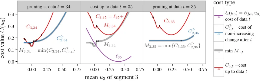
Figure 2: Demonstration of GPDPA for the PeakSeg model (13) withk = 3segments. Cost functions are stored as piecewise functions on intervals (black dots show limits between function pieces). Left: the minM3,34 is the

minimum of two functions:C₂≥_,₃₄is the cost if the second segment ends at data pointt = 34(the min-more operator forces a non-increasing change after), andC3,34is the cost if the second segment ends before that.Middle: the cost C3,35 is the sum of the minM3,34 and the cost of the next data point`35. Right: in the next step, all previously considered changepoints are pruned (costC3,35), since the model with a the second segment ending at data point

t= 35is always less costly (C₂≥_,₃₅).

Note that the minimum of this function is achieved atµ= 1.5which occurs in the first of the two function pieces (red curve on right of Figure 1), with an equality constraint active. This implies the optimal model up to data pointt= 2 withk= 2non-decreasing segment means actually has no change (u1 =u2 = 1.5). In contrast, the minimum of the cost computed by the unconstrained algorithm is atu2 = 1(grey curve on right of Figure 1), resulting in a change down fromu1= 2.

4.4 The PeakSeg up-down constraint

The PeakSeg model described by Hocking et al. [2015] is the most likely segmentation where the first change is up, all up changes are followed by down changes, and all down changes are followed by up changes. More precisely, the constrained optimization problem can be stated as

minimize u∈RK

0=t0<t1<···<tK−1<tK=n

K

X

k=1

htk−1,tk(uk) (13)

subject to uk−1≤uk∀k∈ {2,4, . . .},

uk−1≥uk∀k∈ {3,5, . . .}.

Our proposed Generalized Pruned Dynamic Programming Algorithm (GPDPA) can be used to solve the PeakSeg problem. The initializationk= 1is the same as in the reduced isotonic regression solver (Section 4.2). The dynamic programming updates for evenk∈ {2,4, . . .}are also the same. However, to constrain non-increasing changes, the updates for oddk∈ {3,5, . . .}are

Ck,t(µ) =`(yt, µ) + min{Ck≥−1,t−1(µ), Ck,t−1(µ)}, (14) where the min-more operator is defined for any functionf : _R → _Ras f≥(µ) = minx≥µf(x). Figure 2 shows

(9)

4.5 General affine inequality constraints between adjacent segment means

In this section we briefly discuss how our proposed Generalized Pruned Dynamic Programming Algorithm (GPDPA) can be used to solve any optimization problem with affine inequality constraints between adjacent segment means. For each changek∈ {1, . . . , K−1}, letak, bk, ck∈Rbe arbitrary coefficients that define affine functionsgk(uk, uk+1) = akuk+bkuk+1+ck. The changepoint detection problem with general affine constraints is

minimize u∈RK

0=t0<t1<···<tK−1<tK=n

K

X

k=1

htk−1,tk(uk) (15)

subject to ∀k∈ {1, . . . , K−1}, gk(uk, uk+1)≤0. Some examples of models that are special cases:

1. If we take allak, bk, ck = 0then the constraints are trivially satisfied, we recover the unconstrained segment

neighborhood problem (2).

2. If we take allak = 1,bk=−1andck= 0we recover the reduced isotonic regression problem (5).

3. For the PeakSeg problem (13), we take allck = 0. For oddk∈ {1,3, . . .}we takeak = 1,bk =−1and for

evenk∈ {2,4, . . .}we takeak=−1,bk= 1.

To solve these problems, we need to compute the analog of the min-less/more operator, which we call the constrained minimization operator. For any cost functionf : _R → _Rand constraint functiong : _R×_R → _R, we define the constrained minimization operatorfg_:

R→Ras

fg(uk) = min uk−1:g(uk−1,uk)≤0

f(uk−1). (16)

Whengis affine, the constrained minimization operator is either non-decreasing or non-increasing. In this case it can be computed using a simple algorithm that scans the piecewise functionfeither from left to right or right to left. When a local minimum is found, its value is recorded, and a constant function piece is added (for details see pseudocode for MinLess algorithm in Section B.2). The constrained minimization operator is used in the following general dynamic programming update rule which can be used to compute the solution to (15)

Ck,t(µ) =`(yt, µ) + min{Ck,t−1(µ), C

gk−1

k−1,t−1(µ)}. (17) We note that this update rule is valid for constraint functionsg more general than affine functions. However, the closed-form computation of the constrained minimization operator (16) would possibly be much more difficult for these more general constraint functions (e.g. quadratic constraint functions).

5 Results on peak detection in ChIP-seq data

The real data analysis problem that motivates this work is the detection of peaks in ChIP-seq data [Bailey et al., 2013], which are typically represented as a vector of non-negative countsy ∈ _Zn

+ of aligned sequence reads forn continguous bases in a genome. Data sizes are between n = 105 _{(maximum of the benchmark we consider) and} n= 108_{(largest region with no gaps in the human genome hg19). A peak detector can be represented as a function} c(y)∈ {0,1}n_{for binary classification at every base position. The positive class is peaks (genomic regions with large}

values, representing protein binding or modification) and the negative class is background noise (small values). In the supervised learning framework of Hocking et al. [2016], a data set consists of m count data vectors

y1, . . . ,ymalong with labelsL1, . . . , Lmthat identify regions with and without peaks. Briefly, the number of

er-rorsE[c(yi), Li]is the total of false positives (negative labels with a predicted peak) plus false negatives (positive

(10)

max

median, inter-quartile range

10 100 253

1000 10000

87 263169

n= data points to segment (log scale)

I

=

interv

als

stored

(log

scale)

1 second 1 minute 1 hour

GPDPA

O(nlogn)

PDPA

O(nlogn)

CDPA

O(n2₎

1 100 10000

1000 10000

87 263169

n= data points to segment (log scale)

seconds

(log

[image:10.612.88.541.75.194.2]

scale)

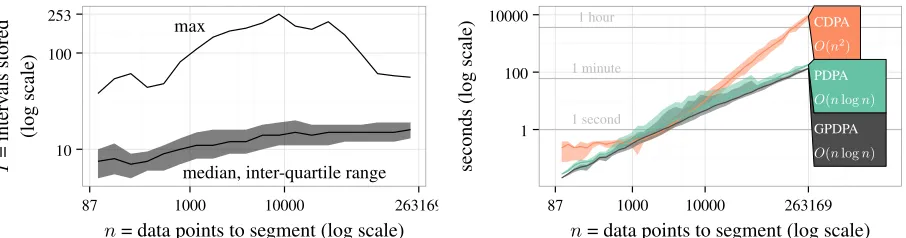
Figure 3: Empirical speed analysis on 2752 count data vectors from the histone mark ChIP-seq benchmark. For each vector we ran the GPDPA with the up-down constraint and a max ofK= 19segments. The expected time complexity isO(KnI)whereIis the average number of intervals (function pieces; candidate changepoints) stored in theCk,t

cost functions.Left: number of intervals stored isI=O(logn)(median, inter-quartile range, and maximum over all data pointstand segmentsk).Right: time complexity of the GPDPA isO(nlogn)(median line and min/max band).

pattern (experiment type, labeler, cell types). The goal in each data set is to learn the pattern encoded in the labels, and find a classifiercthat minimizes the total number of incorrectly predicted labels in a held-out test set:

minimize

c m

X

i=1

E[c(yi), Li]. (18)

Hocking et al. [2015] proposed a constrained dynamic programming algorithm (CDPA) to approximately compute the optimal changepoints, subject to the PeakSeg up-down constraint (Section 4.4). The CDPA has been shown to achieve state-of-the-art peak detection accuracy, by classifying even-numbered segments k as peaks, and odd-numbered segmentskas background noise. However, its quadraticO(Kn2)time complexity makes it too slow to run on large ChIP-seq data sets.

In this section, we show that our proposed GPDPA can be used to overcome this speed drawback, while maintain-ing state-of-the-art accuracy. To show the importance of enforcmaintain-ing the up-down constraint, we consider the uncon-strained Pruned Dynamic Programming Algorithm (PDPA) of Rigaill [2010] as a baseline (Table 1). We also compare against two popular heuristics from the bioinformatics literature, in order to demonstrate that constrained optimization algorithms such as the CDPA and GPDPA are more accurate.

5.1 Empirical time complexity in ChIP-seq data

The ChIP-seq benchmark consists of seven labeled histone data sets. Overall there are 2752 count data vectorsyito

segment, varying in size fromn = 87ton = 263169data. For each count data vectoryi, we ran each algorithm

(CDPA, PDPA, GDPDA) with a maximum ofK = 19segments. This implies a maximum of 9 peaks (one for each even-numbered segment), which is more than enough in these relatively small data sets. To analyze the empirical time complexity, we recorded the number of intervals stored in the Ck,t cost functions (Section 4), as well as the

computation time in seconds.

As in the PDPA, the time complexity of our proposed GPDPA is O(KnI), which depends on the number of intervalsI(candidate changepoints) stored in theCk,tcost functions [Rigaill, 2015]. We observed that the number

of intervals stored by the GPDPA increases as a sub-linear function of the number of data pointsn(left of Figure 3). For the largest data set (n = 263169), the algorithm only stored median=16 and maximum=43 intervals. The most intervals stored was 253 for one data set withn= 7776. These results suggest that our proposed GPDPA only stores on averageO(logn)intervals (possible changepoints), as in the original PDPA. The overall empirical time complexity is thusO(Knlogn)forKsegments andndata points.

(11)

Broad H3K36me3 AM immune Broad H3K36me3 TDH immune Broad H3K36me3 TDH other Sharp H3K4me3 PGP immune Sharp H3K4me3 TDH immune Sharp H3K4me3 TDH other Sharp H3K4me3 XJ immune ● ● ● ● ● ● ● ● ● ● ● ● ● ● ● ● ● ● ● ● ● ● ● ● ● ● ● ● ● ● ● ● ● ● ● ● ● ● ● ● ● ● ● ● ● ● ● ● ● ● ● ● ● ● ● ● ● ● ● ● ● ● ● ● ● ● ● ● ● ● ● ● ● ● ● ● ● ● ● ● ● ● ● ● ● ● ● ● ● ● ● ● ● ● ● ● ● ● ● ● ● ● ● ● ● ● ● ● ● ● ● ● ● ● ● ● ● ● ● ● ● ● ● ● ● ● ● ● ● ● ● ● ● ● ● ● ● ● ● ● MACS(popular baseline) HMCanBroad(popular baseline) PDPA(unconstrained baseline) CDPA(previous best) GPDPA(proposed)

0.6 0.8 1 0.6 0.8 1 0.6 0.8 1 0.6 0.8 1 0.6 0.8 1 0.6 0.8 1 0.6 0.8 1

Test AUC (larger values indicate more accurate peak detection)

algor

[image:11.612.88.538.75.184.2]

ithm

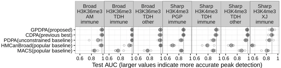
Figure 4: Four-fold cross-validation was used to estimate peak detection accuracy. Each panel shows one of seven ChIP-seq data sets, labeled by experiment (Broad H3K36me3), labeler (AM), and cell types (immune). Each black circle shows test AUC in one of four cross-validation folds, the shaded grey circle is the mean, and the vertical line is the maximum mean in each data set. It is clear that the proposed GPDPA is just as accurate as the previous state-of-the-art CDPA, and both are more accurate than the other baseline methods.

CDPA andO(nlogn)for the PDPA and GPDPA. In agreement with these expectations, our proposed GPDPA shows

O(nlogn)asymptotic timings similar to the PDPA (right of Figure 3).

It is clear that theO(n2₎_{CDPA algorithm is slower than the other two algorithms, especially for larger data sets.} For the largest count data vector (n= 263169), the CDPA took over two hours, but the GPDPA took only about two minutes. Our proposed GPDPA is nearly as fast as MACS [Zhang et al., 2008], a heuristic from the bioinformatics literature which took about 1 minute to compute 10 peak models for this data set.

The total computation time to process all 2752 count data vectors was 156 hours for the CDPA, and only 6 hours for the GPDPA (26 times faster). Overall, these results suggest that our proposed GPDPA enjoysO(nlogn)time complexity in ChIP-seq data, which makes it possible to use for very large data sets.

5.2 Test accuracy in ChIP-seq data

For the optimal changepoint detection algorithms (CDPA, PDPA, GPDPA), the prediction problem simplifies to se-lecting the number of segments Ki ∈ {1,3, . . . ,19} for each data vector i, resulting in a predicted peak vector

cKi₍_y

i)∈ {0,1}n. We select the number of segments using an oracle penaltyKiλ = arg minklik+λoik[Cleynen

and Lebarbier, 2014], wherelik is the Poisson loss andoik is the oracle model complexity for the model with k

segments for data vectori. The problem thus simplifies to learning a scalar penalty constantλ,

minimize

λ m

X

i=1

EhcKiλ₍_y_i₎_{, L}_i

i

. (19)

To demonstrate that changepoint detection algorithms are more accurate than typical heuristics from the bioinfor-matics literature, we also compared with the MACS and HMCanBroad methods [Zhang et al., 2008, Ashoor et al., 2013]. MACS is a popular heuristic for data with a sharp peak pattern such as H3K4me3, and HMCanBroad is a pop-ular heuristic for data with a broad peak pattern such as H3K36me3. Although they are not designed for supervised learning, we trained them by performing grid search over a single significance threshold parameter (qvalue for MACS and finalThreshold for HMCanBroad).

(12)

Since the baseline HMCanBroad algorithm was designed for data with a broad peak pattern, we expected it to perform well in the H3K36me3 data. In agreement with this expectation, HMCanBroad showed state-of-the-art test AUC in two H3K36me3 data sets (broad peak pattern), but was very inaccurate in four H3K4me3 data sets (sharp peak pattern). We expected the baseline MACS algorithm to perform well in the H3K4me3 data sets, since it was designed for data with a sharp peak pattern. In contrast to this expectation, MACS had test AUC values much lower than the optimization-based algorithms in all seven data sets (Figure 4). These results suggest that constrained optimal changepoint detection algorithms are more accurate than the heuristics from the bioinformatics literature.

6 Discussion and conclusions

Algorithms for changepoint detection can be classified in terms of time complexity, optimality, constraints, and pruning techniques (Table 1). In this paper, we investigated generalizing the functional pruning technique originally discovered by Rigaill [2010] and Johnson [2011]. We showed that the functional pruning technique can be used to compute optimal changepoints subject to affine constraints on adjacent segment mean parameters.

We showed that our proposed Generalized Pruned Dynamic Programming Algorithm (GPDPA) enjoys the same log-linearO(Knlogn)time complexity as the original unconstrained PDPA, when applied to peak detection in ChIP-seq data sets (Figure 3). However, we observed that the up-down constrained GPDPA is much more accurate than the unconstrained PDPA (Figure 4). These results suggest that the up-down constraint is necessary for computing a changepoint model with optimal peak detection accuracy. Indeed, we observed that the GPDPA enjoys the same state-of-the-art accuracy as the previous best, the relatively slow quadraticO(Kn2₎_{time CDPA.}

We observed that the heuristic algorithms which are popular in the bioinformatics literature (MACS, HMCan-Broad) are much less accurate than the optimal changepoint detection algorithms (CDPA, PDPA, GPDPA). In the past these sub-optimal heuristics have been preferred because of their speed. For example, the CDPA took 2 hours to compute 10 peak models in the largest data set in the ChIP-seq benchmark, whereas the GPDPA took 2 minutes, and the MACS heuristic took 1 minute. Using our proposed GPDPA, it is now possible to compute highly accurate models in an amount of time that is comparable to heuristic algorithms. Our proposed GPDPA can now be used as an optimal alternative to heuristic algorithms, even for large data sets.

For future work we will be interested in exploring pruning techniques for other constrained changepoint models. When the number of expected changepoints grows with the number of data points, thenK=O(n)and our proposed GPDPA hasO(n2logn)average time complexity (since it computes all models with1, . . . , K segments). We have already started modifying the GPDPA for optimal partitioning [Jackson et al., 2005], which results in the Generalized Functional Prunining Optimal Partitioning (GFPOP) algorithm (Section B.5). It computes theK-segment model for a single penalty constantλ(without computing models with1, . . . , K−1segments) inO(nlogn)time.

7 Reproducible Research Statement

The source code and data used to create this manuscript (including all figures) is available athttps://github. com/tdhock/PeakSegFPOP-paper

8 Acknowledgements

(13)

The supplementary materials begin on this page.

A

Proof of optimality of dynamic programming algorithm

In this section we give a proof of Theorem 1.

Proof. Case 1 and 2 follow from the definition ofCK,t(u).

We now focus on case 3. First notice that by definition of CK,t+1(u)(i.e. the optimal segmentation) we must haveCK,t+1(u) ≤ CK,t(u) +`(yt, u)and alsoCK,t+1(u) ≤CK−1,t(u) +`(yt, u). Thus we haveCK,t+1(u) ≤ min{CK,t(u), CK−1,t(u)}+`(yt+1, u).

Now let us assume,

CK,t+1(u)<min{CK,t(u), CK−1,t(u)}+`(yt+1, u). We will show that this lead to a contradiction.

We consider the optimal segmentation(u,t)∈ IK

t+1which achieves the optimum ofCK,t+1(u). We consider two possible cases:

Scenario 1:tK < t. Definet0such that for alli < K, we havet0i =tiandt0K =t. We have(u,t0)∈ I K

t . We can

thus decomposeCK,t+1(u)as

CK,t+1(u) =

K

X

k=1 ht0

k−1,t

0

k(uk) +`(yt+1, u).

By assumption we would recover PK

k=1ht0

k−1,t0k(uk) < CK,t(u) which is a contradiction by definition of CK,t(u).

Scenario 2:tK =t. Definet0such that for alli < K−1, we haveti0 =tiandt0K−1=t. Also defineu0such that for allk≤K−1, we haveu0_k =uk. Thus(u0,t0)∈ ItK−1, and can then decomposeCK,t+1(u)as

CK,t+1(u) =

K

X

k=1 ht0

k−1,t0k(u

0

k) +`(yt+1, u).

By assumption we would recoverPK−1

k=1 ht0

k−1,t

0

k(u

0

k) < CK−1,t(u)which is a contradiction by definition of

CK−1,t(u).

We have thus proved that the dynamic programming update rules can be used for computing the optimal cost functionsCk,t.

B

Algorithm pseudocode

(14)

B.1 GPDPA for reduced isotonic regression

We begin by providing a pseudocode solver for the simplest case, the reduced isotonic regression problem. We propose the following data structures and sub-routines for the computation:

• FunctionPiece: a data structure which represents one piece of aCk,t(u)cost function (for one interval of mean

valuesu). It has coefficients which depend on the convex loss function`(for the square loss it has three real-valued coefficientsa, b, cwhich define a functionau2₊_bu₊_c_{). It also has two real-valued elements for min/max} mean values[u, u]of this interval, meaning the functionCk,t(u) =au2+bu+cfor allu∈[u, u]. Finally it

stores a previous segment endpointt0(integer) and meanu0(real).

• FunctionPieceList: an ordered list of FunctionPiece objects, which exactly stores a cost functionCk,t(u)for all

values of last segment meanu.

• OnePiece(y, u, u): a sub-routine that initializes a FunctionPieceList with just one FunctionPiece`(y, u)defined on[u, u].

• MinLess(t, f): an algorithm that inputs a changepoint and a FunctionPieceList, and outputs the corresponding min-less operatorf≤ (another FunctionPieceList), with the previous changepoint set tot0 =t for each of its pieces. This algorithm also needs to store the previous mean value u0 for each of the function pieces (see pseudocode below).

• MinOfTwo(f1, f2): an algorithm that inputs two FunctionPieceList objects, and outputs another Function-PieceList object which is their minimum.

• ArgMin(f): an algorithm that inputs a FunctionPieceList and outputs three values: the optimal meanu∗ = arg min_uf(u), the previous segment endt0and meanu0.

• FindMean(u, f)an algorithm that inputs a mean value and a FunctionPieceList. It finds the FunctionPiece inf

with meanu∈[u, u]contained in its interval, then outputs the previous segment endt0and meanu0 stored in that FunctionPiece.

The above data structures and sub-routines are used in the following pseudocode, which describes the GPDPA for solving the reduced isotonic regression problem.

Algorithm 1Generalized Pruned Dynamic Programming Algorithm (GPDPA) for solving the reduced isotonic re-gression problem.

1: Input: data sety∈Rn, maximum number of segmentsK∈ {2, . . . , n}.

2: Output: matrices of optimal segment meansU ∈RK×Kand endsT ∈ {1, . . . , n}K×K

3: Compute minyand maxyofy. 4: C1,1←OnePiece(y1, y, y) 5: for data pointstfrom 2 ton:

6: C1,t←OnePiece(yt, y, y) +C1,t−1

7: for segmentskfrom 2 toK: for data pointstfromkton: // dynamic programming 8: min prev←MinLess(t−1, Ck−1,t−1)// this isCk≤−1,t−1

9: min new←min prev ift=k, else MinOfTwo(min prev, Ck,t−1) 10: Ck,t←min new+OnePiece(yt, y, y)

11: for segmentskfrom 1 toK: // decoding for every model sizek

12: u∗, t0, u0 ←ArgMin(Ck,n)

13: Uk,k←u∗;Tk,k←t0// store mean of segmentkand end of segmentk−1

14: for segmentsfromk−1to1: // decoding for every segments < k

15: ifu0<∞:u∗←u0// equality constraint active,us=us+1 16: t0, u0←FindMean(u∗, Cs,t0)

(15)

Algorithm 1 begins by computing the min/max on line 3. The main storage of the algorithm isCk,t, which should

be initialized as a K×n array of empty FunctionPieceList objects. The computation of C1,t for all t occurs on

lines 4–6.

The dynamic programming updates occur in the for loops on lines 7–10. Line 8 uses the MinLess sub-routine to compute the temporary FunctionPieceList min prev (which represents the functionC_k≤₋₁_,t₋₁). Line 9 sets the temporary FunctionPieceList min new to the cost of the only possible changepoint ift = k; otherwise, it uses the MinOfTwo sub-routine to compute the cost of the best changepoint for every possible mean value. Line 10 adds the cost of data pointt, and stores the resulting FunctionPieceList inCk,t.

The decoding of the optimal segment meanU (aK×K array of real numbers) and endT (aK×Karray of integers) variables occurs in the for loops on lines 11–17. For a given model sizek, the decoding begins on line 12 by using the ArgMin sub-routine to solveu∗= arg min_uCk,n(u)(the optimal values for the previous segment endt0

and meanu0 are also returned). Now we know thatu∗ is the optimal mean of the last (k-th) segment, which occurs from data pointt0+ 1ton. These values are stored inUk,kandTk,k(line 13). And we already know that the optimal

mean of segmentk−1isu0. Note that theu0 =∞flag means that the equality constraint is active (line 15). The decoding of the other segmentss < kproceeds using the FindMean sub-routine (line 16). It takes the costCs,t0 of the best model inssegments up to data pointt0, finds the FunctionPiece that stores the cost ofu∗, and returns the new optimal values of the previous segment endt0 _{and mean}_u0_{. The mean of segment}_s_{is stored in}_U

k,sand the end of

segments−1is stored inTk,s(line 17).

The time complexity of Algorithm 1 isO(KnI)whereIis the complexity of the MinLess and MinOfTwo sub-routines, which is linear in the number of intervals (FunctionPiece objects) that are used to represent the cost functions. There are pathological synthetic data sets for which the number of intervalsI=O(n), implying a time complexity of

O(Kn2_{). However, the average number of intervals in real data sets is empirically}_I₌_O_(log_n_{), so the average time} complexity of Algorithm 1 isO(Knlogn).

B.2 MinLess algorithm

The MinLess algorithm implements the min-less operatorf≤(Definition 3), which is an essential sub-routine of the GPDPA. The following sub-routines are used to implement the MinLess algorithm.

• GetCost(p, u): an algorithm that takes a FunctionPiece objectp, and a mean valueu, and computes the cost at

u. For a square loss FunctionPiecepwith coefficientsa, b, c∈R, we have GetCost(p, u) =au2+bu+c.

• OptimalMean(p): an algorithm that takes one FunctionPiece object, and computes the optimal mean value. For a square loss FunctionPiecepwe have OptimalMean(p) =−b/(2a).

• ComputeRoots(p, d): an algorithm that takes one FunctionPiece object, and computes the solutions top(u) =d. For the square loss we propose to use the quadratic formula. For other convex losses that do not have closed form expressions for their roots, we propose to use Newton’s root finding method. Note that for some constants

dthere are no roots, and the algorithm needs to report that.

• f.push piece(u, u, p, u0): push a new FunctionPiece at the end of FunctionPieceListf, with coefficients defined by FunctionPiecep, on interval[u, u], with previous segment mean set tou0.

• ConstPiece(c): sub-routine that initializes a FunctionPiecepwith constant costc (for the square loss it sets

(16)

Algorithm 2MinLess algorithm.

1: Input: The previous segment endtprev(an integer), andfin(a FunctionPieceList). 2: Output: FunctionPieceListfout, initialized as an empty list.

3: prev cost← ∞

4: new lower limit←LowerLimit(fin[0]). 5: i←0; // start at FunctionPiece on the left

6: whilei <Length(fin): // continue until FunctionPiece on the right 7: FunctionPiecep←fin[i]

8: if prev cost =∞: // look for min in this interval. 9: candidate mean←OptimalMean(p)

10: if LowerLimit(p)<candidate mean<UpperLimit(p):

11: new upper limit←candidate mean // Minimum found in this interval. 12: prev cost←GetCost(p,candidate mean)

13: prev mean←candidate mean

14: else: // No minimum in this interval. 15: new upper limit←UpperLimit(p)

16: fout.push piece(new lower limit,new upper limit, p,∞) 17: new lower limit←new upper limit

18: i←i+ 1

19: else: // look for equality ofpand prev cost

20: (small root,large root)←ComputeRoots(p,prev cost) 21: if LowerLimit(p)<small root<UpperLimit(p):

22: fout.push piece(new lower limit,small root,ConstPiece(prev cost),prev mean) 23: new lower limit←small root

24: prev cost← ∞

25: else: // no equality in this interval

26: i←i+ 1// continue to next FunctionPiece 27: if prev cost<∞: // ending on constant piece

28: fout.push piece(new lower limit,UpperLimit(p),ConstPiece(prev cost),prev mean) 29: Set all previous segment endt0₌_t

prevfor all FunctionPieces infout

Consider Algorithm 2 which contains pseudocode for the computation of the min-less operator. The algorithm initializes prev cost (line 3), which is a state variable that is used on line 8 to decide whether the algorithm should look for a local minimum or an intersection with a finite cost. Since prev cost is initially set to∞, the algorithm begins by following the convex function pieces from left to right until finding a local minimum. If no minimum is found in a given convex FunctionPiece (line 15), it is simply pushed on to the end of the new FunctionPieceList (line 16). If a minimum occurs within an interval (line 10), the cost and mean are stored (lines 11–12), and a new convex FunctionPiece is created with upper limit ending at that mean value (line 16). Then the algorithm starts looking for another FunctionPiece with the same cost, by computing the smaller root of the convex loss function (line 20). When a FunctionPiece is found with a root in the interval (line 21), a new constant FunctionPiece is pushed (line 22), and the algorithm resumes searching for a minimum. At the end of the algorithm, a constant FunctionPiece is pushed if necessary (line 28). The complexity of this algorithm isO(I)whereIis the number of FunctionPiece objects infin.

The algorithm which implements the min-more operator is analogous. Rather than searching from left to right, it searches from right to left. Rather than using the small root (line 21), it uses the large root.

B.3 Implementation details

Some implementation details that we found to be important:

(17)

Segment Neighborhood Optimal Partitioning

unconstrained PDPA FPOP

[image:17.612.172.442.72.110.2]

constrained GPDPA GFPOP

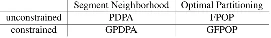
Table 2: Algorithms for solving constrained and unconstrained versions of the Segment Neighborhood and Optimal Partitioning problems. PDPA = Pruned Dynamic Programming Algorithm, FPOP = Functional Pruning Optimal Partitioning, G = Generalized (can handle affine constraints on adjacent segment means).

n = 4countsyt5,1,0,5 with corresponding weights wt1,3,2,2 then the Poisson loss function for meanµis

`(yt, wt, µ) =wt(µ−ytlogµ).

Mean cost The text definesCk,tfunctions as the total cost. However for very large data sets the cost values will be

very large, resulting in numerical instability. To overcome this issue we instead implemented update rules using the mean cost. For weightsWt=P

t

i=1wi, the update rule to compute the mean cost is

Ck,t(µ) =

1

Wt

h

`(yt, µ) +Wt−1min{Ck,t−1(µ), Ck≤−1,t−1(µ)}

i

Intervals in log(mean) space For the Poisson model of non-negative count datayt∈ {0,1,2, . . .}there is no

possi-ble meanµvalue less than 0. We thus usedlog(µ)values to implement intervals in FunctionPiece objects. For example rather than storingµ∈[0,1]we storelogµ∈[−∞,0].

Root finding For the ComputeRoots sub-routine for the Poisson loss, we used Newton root finding. For the larger root we solvealogµ+bµ+c = 0(linear asµ → ∞) and for the smaller root we solveax+bex₊_c _{= 0}

(x= logµ, linear asx→ −∞andµ→0). We stop the root finding when the cost is near zero (absolute cost value less than10−12_).

Storage Since the dynamic programming update rule forCk,tonly depends onC_k≥₋₁_,t₋₁ andCk,t−1, these are the only functions that need to be in memory, and the rest of the cost functions can be stored on disk (until the decoding step). We used the Berkeley DB Standard Template Library to store all theCk,tas a vector of

Func-tionPieceList objects.

B.4 Penalized version of reduced isotonic regression

Maidstone et al. [2016] proposed the Functional Pruning Optimal Partitioning (FPOP) algorithm to solve the “penal-ized” or “optimal partitioning” version of the segment neighborhood problem, where the constraint ofKsegments is replaced by a non-negative penaltyλ∈R+on the number of changes in the objective function. Rather than computing all models from 1 toKsegments (as in the PDPA), the FPOP algorithm computes the single model withKsegments (without computing models from 1 toK−1segments). The same penalization idea can be applied to models with affine constraints between adjacent segment means. The penalized version of the reduced isotonic regression problem (3) can be stated as

minimize m∈Rn

c∈{0,1}n−1

n

X

t=1

`(yt, mt) +λ n−1

X

t=1

I(ct6= 0) (20)

subject to ct= 0⇒mt=mt+1 ct= 1⇒mt≤mt+1.

Note that thectvariable is a changepoint indicator. The same functional pruning techniques used for the GPDPA can

(18)

LetCλ,t(u)be the penalized cost of the most likely segmentation up to data pointt, with last segment meanu.

The initialization for the first data point isCλ,1(u) = `(y1, u). The dynamic programming update rule for all data pointst >1is

Cλ,t(u) =`(yt, u) + min{C

≤

λ,t−1(u) +λ, Cλ,t−1(u)}. (21) The same sub-routines described in Section B.2 can be used to implement the algorithm below, which solves the penalized reduced isotonic regression problem (20).

Algorithm 3Generalized Functional Pruning Optimal Partitioning (GFPOP) for penalized reduced isotonic regression

1: Input: data sety∈Rn, penalty constantλ≥0.

2: Output: vectors of optimal segment meansU ∈Rnand endsT ∈ {1, . . . , n}n

3: Compute minyand maxyofy.

4: Cλ,1←OnePiece(y1, y, y)

5: for data pointstfrom 2 ton: // dynamic programming 6: min prev←λ+MinLess(t−1, Cλ,t−1)

7: min new←MinOfTwo(min prev, Cλ,t−1) 8: Cλ,t←min new+OnePiece(yt, y, y)

9: u∗, t0, u0 ←ArgMin(Cλ,n)// begin decoding

10: i←1;Ui←u∗;Ti←t0

11: whilet0>0:

12: ifu0<∞:u∗←u0

13: t0, u0←FindMean(u∗, Cλ,t0) 14: i←i+ 1;Ui←u∗;Ti ←t0

Algorithm 3 begins by computing the min/max (line 3). The main storage of the algorithm isCλ,t, which should

be initialized as an array ofnempty FunctionPieceList objects.

The dynamic programming recursion in this algorithm has only one for loop over data pointst(line 5). The penalty constantλis added to all of the function pieces that result from MinLess (line 6), before computing MinOfTwo (line 7). The last step of each dynamic programming update is to add the cost of the new data point (line 8).

The decoding process on lines 9–14 is essentially the same as the GPDPA (Algorithm 1). The last segment mean and second to last segment end are first stored on line 10 in(U1, T1). For each other segmenti, the mean and previous segment end are stored on line 14 in(Ui, Ti). Note that there should be space to store(Ui, Ti)parameters for up ton

segments. However, there are usually less thannsegments, and the algorithm should return a special flag for unused parameters, for example(Ui=∞, Ti=−1).

The time complexity of Algorithm 3 isO(nI), where Iis the time complexity of the MinLess and MinOfTwo sub-routines. As in the GPDPA, the time complexity of these sub-routines is linear in the number of intervals (Func-tionPiece objects) that are used to represent theCλ,t cost functions. Since the number of intervals in real data is

typicallyI=O(logn)(see Section 5.1), the overall time complexity of Algorithm 3 is on averageO(nlogn).

B.5 Generalized Functional Pruning Optimal Partitioning Solvers

The GFPOP algorithm can solve problems with more general constraints than reduced isotonic regression. LetG= (V, E)be a directed graph that represents the model constraints (for examples see Figure 5). The vertices V =

(19)

Unconstrained 1

g0, λ

Reduced isotonic regression

1

g↑, λ

Peak detection

peak

background g↑, λ↑ g↓, λ↓

Unimodal regression

up/down

up _down

g↑, λ1

g↑, λ2

g↓, λ3

[image:19.612.89.543.73.208.2]

g↓, λ4

Figure 5: Examples of state graphs for four models. Nodes represent states and edges represent changes. Each change has a corresponding penaltyλ, and a functiongthat determines what types of changes are possible (g0any change,g↑ non-decreasing,g↓non-increasing). Even if there is no edge from a node to itself, it is still possible to stay in the same state without introducing a changepoint and penalty. Note that the Unimodal regression state X should be interpreted as “can change X” e.g. up/down means “can change up/down.”

Reduced Isotonic Regression

C1,t C1,t+1

C1,t

Cg↑

1,t+λ

Peak detection

Cpeak,t

Cbkg,t

Cpeak,t+1

Cbkg,t+1

Cpeak,t

C_peakg↓,t+λ↓

Cbkg,t

Cg↑

bkg,t+λ↑

Unimodal regression

Cup,t

Cup/down,t

Cdown,t

Cup,t+1

Cup/down,t+1

Cdown,t+1

Cup,t

Cup/down,t

Cdown,t

Cg↑

up,t+λ1

C_up/downg↑ _,t+λ2

Cg↓

up/down,t+λ3

Cg↓

down,t+λ4

Figure 6: Computation graphs which represent the dynamic programming updates (23) for the state graph models in Figure 5. Nodes represent cost functions Cs,t in each state s at data t and t+ 1. Edges represent inputs to

the min{} operation (solid for a changepoint, dotted for no change). For example in reduced isotonic regression,

C1,t+1(u) =`(yt+1, u) + min{C1,t(u), C g↑

1,t(u) +λ}.

In the optimization problem below we also allowc= 0, which implies no penaltyλ0= 0, and means no change:

minimize m∈Rn,s∈Vn

c∈{0,1,...,|E|}n−1

n

X

t=1

`(yt, mt) + n−1

X

t=1

λct (22)

subject to ct= 0⇒mt=mt+1andst=st+1

[image:19.612.93.523.293.530.2]

(20)

If some states are desired at the start or end, then those constraintss1∈S, sn ∈Scan also be enforced. To compute

the solution to this optimization problem, we propose the following dynamic programming algorithm.

LetCs,t(u)be the optimal cost with meanuand statesat data pointt. This quantity can be recursively computed

using dynamic programming. The initialization for the first data point isCs,1(u) = `(y1, u)for all statess. The dynamic programming update rule for all data pointst >1is

Cs,t(u) =`(yt, u) + min{Ms,t−1(u), Cs,t−1(u)}, (23) where the minimum cost of all possible changes to statesfrom time pointt−1is

Ms,t−1(u) = min

c∈Es Cgc

v_c,t−1(u) +λc, (24)

and the set of all changes going to statesis

Es={c∈E|vc=s}. (25)

The computations required for the dynamic programming updates (23) can be visualized using a computation graph (Figure 6).

The pseudocode for the algorithm which implements the dynamic programming updates (23) is stated below.

Algorithm 4Generalized Functional Pruning Optimal Partitioning Algorithm, Dynamic Programming (GFPOP-DP)

1: Input: datayand weightsw(both sizen), number of vertices/states|V|, startsS⊆V, edges/transitionsE. 2: Allocate|V| ×narray of optimal cost functionsCs,t, each initialized to NULL.

3: fortfrom1ton: 4: ift== 1:

5: forsinS: // initialize cost for all possible starting states 6: Cs,t←InitialCost(yt, wt)

7: else:

8: forsfrom1to|V|:

9: ifCs,t−1is NOT NULL: // previous cost in this state has been computed 10: Cs,t←Cs,t−1// cost of staying in this state (no change)

11: for (v,v,λ, ConstrainedCost) inE:

12: ifCv,t−1is NOT NULL: // previous cost has been computed 13: cost of change←ConstrainedCost(Cv,t−1)

14: cost of change.set(v, t−1) 15: cost of change.addPenalty(λ)

16: ifCv,tis NULL:

17: Cv,t←cost of change

18: else:

19: Cv,t←MinOfTwo(Cv,t,cost of change)

20: forsfrom1to|V|: 21: ifCs,tis NOT NULL:

22: Cs,t.addDataPoint(yt, wt)

23: Output:|V| ×narray of optimal cost functionsCs,t.

The algorithm above performs several checks ifCs,tis NULL or not (lines 9, 12, 16, 21). All costs are initialized

as NULL (line 2). After having performed the cost update for datat, a NULL costCs,tmeans that statesis not feasible

at datat. For each constraint functiong there is a corresponding ConstrainedCost sub-routine that is mentioned on lines 11 and 13 (e.g. no constraintg0MinUnconstrained, non-decreasing changeg↑MinLess, non-increasing change

g↓MinMore).

(21)

in the empirical tests of the peak detection model on ChIP-seq data (Section 5.1), so we expect that the average time complexity of Algorithm 4 isO(|V|nlogn).

Note that the algorithm above only performs the dynamic programming. The decoding of optimal model parame-ters is achieved using the algorithm below.

Algorithm 5Generalized Functional Pruning Optimal Partitioning Algorithm, decoding (GFPOP-decode)

1: Output:|V| ×narray of optimal cost functionsCs,t, endsS⊆V.

2: Allocatem∈Rn(mean),s∈Zn(state),t∈Zn(segment end).

3: u∗, s∗, t0, s0 ←ArgMin(C·,n, S)// begin decoding

4: i←1;mi←u∗;si←s∗; ti←n

5: whilet0>0: 6: i←i+ 1;ti←t0

7: u∗, s∗, t0, s0 ←ArgMin(Cs0_,t0) 8: mi ←u∗;si←s∗

9: Output:m,s,t.

References

H. Ashoor, A. H´erault, A. Kamoun, F. Radvanyi, V. Bajic, E. Barillot, and V. Boeva. HMCan: a method for detecting chromatin modifications in cancer samples using ChIP-seq data.Bioinformatics, 29(23):2979–2986, 2013.

I. Auger and C. Lawrence. Algorithms for the optimal identification of segment neighborhoods. Bull Math Biol, 51: 39–54, 1989.

T. Bailey, P. Krajewski, I. Ladunga, C. Lefebvre, Q. Li, T. Liu, P. Madrigal, C. Taslim, and J. Zhang. Practical guidelines for the comprehensive analysis of ChIP-seq data.PLoS computational biology, 9(11), 2013.

R. Bellman. On the approximation of curves by line segments using dynamic programming. Commun. ACM, 4(6): 284–, June 1961.

M. Best and N. Chakravarti. Active set algorithms for isotonic regression; a unifying framework. Mathematical Programming, 47(1):425–439, 1990.

N. Haiminen, A. Gionis, and K. Laasonen. Algorithms for unimodal segmentation with applications to unimodality detection.Knowledge and Information Systems, 14(1):39–57, 2008.

J. Hardwick and Q. Stout. Optimal reduced isotonic regression.arXiv preprint arXiv:1412.2844, 2014.

T. Hocking, G. Rigaill, and G. Bourque. PeakSeg: constrained optimal segmentation and supervised penalty learning for peak detection in count data. InProc. 32nd ICML, pages 324–332, 2015.

T. Hocking, P. Goerner-Potvin, A. Morin, X. Shao, T. Pastinen, and G. Bourque. Optimizing chip-seq peak detectors using visual labels and supervised machine learning. Bioinformatics, 2016.

H. Hoefling. A path algorithm for the fused lasso signal approximator. Journal of Computational and Graphical Statistics, 19(4):984–1006, 2010.

B. Jackson, J. Scargle, D. Barnes, S. Arabhi, A. Alt, P. Gioumousis, E. Gwin, P. Sangtrakulcharoen, L. Tan, and T. Tsai. An algorithm for optimal partitioning of data on an interval.IEEE Signal Process Lett, 12:105–108, 2005.

N. Johnson. Efficient models and algorithms for problems in genomics. PhD thesis, Stanford, 2011. https://purl.stanford.edu/jq411pj0455.

(22)

R. Killick, P. Fearnhead, and I. Eckley. Optimal detection of changepoints with a linear computational cost.

arXiv:1101.1438, Jan. 2011.

R. Maidstone, T. Hocking, G. Rigaill, and P. Fearnhead. On optimal multiple changepoint algorithms for large data.

Statistics and Computing, pages 1–15, 2016. ISSN 1573-1375.

P. Mair, K. Hornik, and J. de Leeuw. Isotone optimization in R: pool-adjacent-violators algorithm (PAVA) and active set methods.Journal of statistical software, 32(5):1–24, 2009.

A. Cleynen and E. Lebarbier. Segmentation of the Poisson and negative binomial rate models: a penalized estimator.

ESAIM: PS, 18:750–769, 2014.

G. Rigaill. Pruned dynamic programming for optimal multiple change-point detection. arXiv:1004.0887, 2010.

G. Rigaill. A pruned dynamic programming algorithm to recover the best segmentations with 1 to kmax change-points.

Journal de la Société Française de la Statistique, 156(4), 2015.

G. Rote. Isotonic regression by dynamic programming.

http://www.inf.fu-berlin.de/lehre/WS12/HA/isotonicregression.pdf, unpublished.

M. Schell and B. Singh. The reduced monotonic regression method. Journal of the American Statistical Association, 92(437):128–135, 1997.

A. Scott and M. Knott. A cluster analysis method for grouping means in the analysis of variance. Biometrics, 30: 507–512, 1974.

R. Tibshirani, H. Hoefling, and R. Tibshirani. Nearly-isotonic regression. Technometrics, 53(1):54–61, 2011.

A log linear time algorithm for constrained changepoint detection