Using Recurrent Neural Networks
Spyros Boukoros1, Anupiya Nugaliyadde2, Angelos Marnerides3, Costas Vassilakis4, Polychronis Koutsakis2, and Kok Wai Wong 2
1Department of Computer Science, Technische Universität Darmstadt, Germany 2School of Engineering and Information Technology, Murdoch University, Australia
3School of Computing and Communications, Lancaster University, UK 4Department of Informatics and Telecommunications, University of Peloponnese, Greece [email protected], {a.nugaliyadde, p.koutsakis,
k.wong}@mur-doch.edu.au, [email protected], [email protected]
Abstract. As email workloads keep rising, email servers need to handle this ex-plosive growth while offering good quality of service to users. In this work, we focus on modeling the workload of the email servers of four universities (2 from Greece, 1 from the UK, 1 from Australia). We model all types of email traffic, including user and system emails, as well as spam. We initially tested some of the most popular distributions for workload characterization and used statistical tests to evaluate our findings. The significant differences in the prediction accu-racy results for the four datasets led us to investigate the use of a Recurrent Neu-ral Network (RNN) as time series modeling to model the server workload, which is a first for such a problem. Our results show that the use of RNN modeling leads in most cases to high modeling accuracy for all four campus email traffic datasets.
Keywords: Email Traffic, Model Server Workload, Recurrent Neural Network, Time Series Modeling.
1
Introduction
it becomes a matter of crucial importance that servers can cope with the heavy workload and do not crash or exhibit degraded email delivery performance.
All of the above facts, regarding regular and spam email traffic show the urgent need for accurate email traffic prediction, which will help system administrators to take ac-tions to optimize the way they allocate the storage space, processing resources or the bandwidth that they have at their disposal. By doing so, they will be able to avoid sys-tem crashes and failures and offer users a better quality of service. Gomez et al.[4] found that message sizes could be represented by lognormal distributions at the body and the tail. Their measurement period was one week. They also modeled the arrival process and the popularity of various email receivers. The Poisson arrival process was shown to fit their workload. The popularity of objects was modeled with a Zipf-like distribution. Bertolotti and Calzarossa [5] also collected the SMTP logs from email servers and modeled the workload. They modeled the message sizes, interarrival times and the number of recipients. The lognormal distribution was found to be the best fit for the message sizes. The interarrival times were shown to fit Weibull and Pareto dis-tributions, in contrast with the conclusions in [4]. In [6] Shah and Noble present a large-scale study on an email server. They model various parameters from the message sizes to the number of words emails consist of. Their measurement period lasted more than 7 months. Regarding the modeling of message sizes, which is the focus of this study, they noticed that the cumulative distribution function (CDF) is symmetric under log scale. Hence, they concluded in this empirical way that their data must be distributed with a lognormal distribution. The main body was modeled with a lognormal distribu-tion while the tail was modeled with a Pareto, following the lead of [4]. In this way, the workload was modeled with high accuracy. While [4] found that spam emails have smaller sizes than regular ones, [6] claims the opposite. However, both of the above studies concluded that spam traffic is distributed with a lognormal distribution. Paxson modeled wide–area transport Layer Protocol (TCP) connections [7]. SMTP connec-tions are TCP connecconnec-tions for transferring emails. Unlike the previously mentioned studies and in accordance to our work he used goodness of fit tests to back up his find-ings. Regarding the SMTP connections, he found that the empirical distribution was bimodal and justified that from the fact that users sent either simple text mail or files. He decided to model it with two lognormal distributions, breaking the data in two pop-ulations, one below the 80th percentile and the other above.
However, as it will be explained in the following sections, when evaluating the same methodology over three new datasets from other universities, we found that the predic-tion accuracy was smaller. For this reason, we decided to use a Recurrent Neural Net-work (RNN) and treat this as a time series problem.
To the best of our knowledge from the literature review, this is the first time that RNN is used for modeling email traffic, and the use of time series modeling for email size prediction is proposed for the first time as well. We anticipated that time series modeling could be an option given that the email traffic can be viewed as a series of events over a time period. The email traffic prediction accuracy with the use of the RNN time series prediction was found to be substantially higher, for all four datasets, than the probabilistic modeling approach.
The only work in the literature that is slightly relevant to our work is the study in [14], where the authors try to extract information from individual email histories, fo-cusing on understanding how an individual communicates over time with recipients in their social network.
2
Methodology
2.1 Data Collection and Processing
With the invaluable help of academic colleagues and of the technical staff of four uni-versities, we have collected a vast amount of email logs. The four universities were the Technical University of Crete (TUC), Greece, the University of Peloponnese (UoP), Greece, Murdoch University, Australia and Liverpool John Moores University (LJMU), UK.
We got two separate kinds of logs, for the spam and the spam emails. The non-spam emails are the emails that arrived at the server and were not stopped by the filter or classified later as spam. The spam traffic that is blocked from the anti-spam filter is not recorded because the connection is closed before the email actually arrives. The emails that arrive at the servers but are classified as spam are saved into folders with their whole body.
We decided to break our data into 4 categories depending on whether they represent system or users’ emails, and whether they are incoming or outgoing. The system emails consist mainly of server to server communication or diagnostic emails as well as no-reply messages sent to various users. The decision to break the data into categories was based on the fact that the system emails are sent out in bulk, usually to the whole uni-versity to inform everyone about events. Therefore, these emails are of a different na-ture, so we decided to consider them as a different category and model them separately, to achieve higher accuracy.
2.2 Modeling with probability distributions
We wanted to study whether our servers' workloads could be modeled with any of the well-known, from the literature, distributions for workload characterization and mod-eling. This approach serves as an implicit comparison of our conclusions with those of the previous works in the literature, on email traffic modeling. We should mention that the email datasets for those works were not available, to the best of our knowledge, for a direct comparison. The only email corpuses that are available on the web contain actual text from emails, to be used for linguistic analysis. Hence, we relied on our four datasets, which were significantly large.
We used the maximum likelihood estimation method to obtain the parameters which lead the distributions to produce size populations with the same mean and standard deviation as those for each week of our study. The distributions used were the uniform, exponential, gamma, weibull, log-logistic, lognormal and Generalized Extreme Value (GEV). The maximum likelihood estimation method returns a vector with the estimated parameters at the 95% significance level. Simulations were run in Matlab.
2.3 Time Series Modeling using Recurrent Neural Network
As explained in Section 1, we used Recurrent Neural Network (RNN) for creating the model and treated the problem as a time series prediction. We combined all the weeks, except one, for each category separately and tried to predict the last week’s email traffic sizes. We assumed that the data in different weeks have time series patterns that can be used to predict the remaining part of the dataset.
A RNN simulates a discrete dynamic system that has input (Xt), output (Yt) and hid-den layers [15]. In general, a RNN takes the input sequence to the hidhid-den layers to work out the information about the history of all the past elements. As a result, the output of the hidden layers can have some form of discrete time series similar to the output of the deep multilayer networks. The idea of RNN is that it can connect prior information to the present task, such as using previous data sequences to inform the understanding of the present data sequence to predict future data sequences.
Längkvist et al., [16] discuss various techniques using deep learning for time series as well as the recursive strategies performance in time series. Rather et al. [17] show the use of a traditional Recurrent Neural Network (RNN) with a hybrid model to achieve high time series prediction. The time series predictions are based on previous data, where memory networks and recurrent networks have a higher efficiency than any other deep learning method [18].
3
Statistical Tests
We used five statistical tests to evaluate the accuracy of our two main approaches (prob-abilistic and RNN time series).
The first test is the Q-Q plot, a powerful goodness-of-fit test [9] which graphically compares two datasets in order to determine whether the datasets come from popula-tions with a common distribution (if they do, the points of the plot should fall approxi-mately along a 45 degree reference line). More specifically, a Q–Q plot is a plot of the quantiles of the data versus the quantiles of the fitted distribution. A z-quantile of X is any value x such that P((X ≤ x) = z. We have plotted the quantiles of the real data with the respective quantiles of the various distribution fits.
The second test is the Kolmogorov–Smirnov (KS) test [10], which tries to determine if two datasets differ significantly. The KS-test has the advantage of making no as-sumption about the distribution of data, i.e., it is non-parametric and distribution-free. The KS-test uses the maximum vertical deviation between the two curves as its statistic D.
The third test is the Anderson-Darling (AD) test [8], which is a modification of the Kolmogorov-Smirnov test. It places more weight to the tails in comparison to the K-S Test. The test statistic belongs, like the Kolmogorov-Smirnov test, to the family of quadratic empirical distribution function statistics, which measure the distance between the hypothesized and the empirical CDF.
The fourth test is the Kullback-Leibler (KL) Divergence test [11] which measures the information loss between two distributions.
It indicates how many extra bits we are going to need if we code samples using the Q probability distribution function instead of P. The test is non-symmetric meaning that if we reverse the P and Q (probability distributions functions) we get different results. The fifth test is the Relative Percentage Error (RPE) [12], which gives a metric on how different one population is from another. By measuring the absolute difference between the two populations, we do not discriminate which one is bigger or smaller. Of course, we wish to achieve results as close to 0% as possible in order to find a mod-eling approach that has high accuracy.
RPE is defined as: !"# =|&'(|( ∗ 100%,
where Y is the predicted value and X the real observation.
4
Results
4.1 Incoming Traffic for Users
Table 1. Incoming Users Emails' Numbers and Total Size
Min
#emails #emails Max Gbytes Min Gbytes Max weeks # of
TUC 72379 134864 4.34 23.87 9
LJMU 142884 359020 11.6 31.3 4
Murdoch 1132 410672 0.03 56.2 52
UoP 37735 51726 2 4.7 4
Our statistical tests agreed that the log-logistic distribution provides the closest fit to our data for Murdoch and TUC, while GEV provided the closest fit to our data for UoP and LJMU. The fact that the KS test and AD test agreed with each other confirmed that the log-logistic/GEV distribution, respectively, is closest to both the tails and the main body of the distribution.
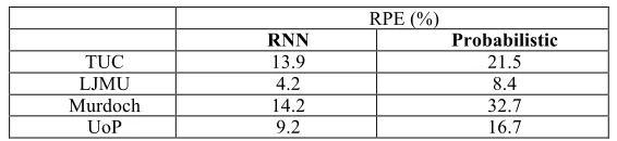
For the probabilistic approach, we found that the RPE results are significantly dif-ferent between the 98% and the 100% of the quantiles because of the outliers, which tend to have extremely large sizes, something that the distribution methods cannot pre-dict. Therefore, these outliers, usually amounting to 1-2% of our traffic in terms of bytes, cause very large errors. The results presented in Table 2 and for the rest of the paper for the probabilistic modeling approach in this section correspond to 98% of the traffic, excluding the outliers. On the contrary, the results presented throughout the pa-per for RNN have been derived without removing any outliers from the training or testing datasets, since RNN is resilient to the existence of outliers.
As shown in Table 2, despite modeling the whole dataset (including the outliers) RNN is able to largely outperform the probabilistic approach for all datasets, based on the RPE metric.
Table 2. Prediction Error for Incoming Users’ Traffic
RPE (%)
RNN Probabilistic
TUC 13.9 21.5
LJMU 4.2 8.4
Murdoch 14.2 32.7
UoP 9.2 16.7
4.2
Incoming System Traffic
[image:6.595.156.439.470.535.2]Table 3. Incoming System Emails’ Numbers and Total Size
Min
#emails #emails Max Gbytes Min Gbytes Max # of weeks
TUC 49985 318944 0.2 2.1 9
LJMU - - - - -
Murdoch 3149 77686 0.03 6 52
UoP 838 7166 0.003 0.06 4
[image:7.595.195.404.315.372.2]As shown in Table 4, RNN again largely outperforms the probabilistic approach for all datasets, based on the RPE metric.
Table 4. Prediction Error for Users’ Incoming System Traffic
RPE (%)
RNN Probabilistic
TUC 2.1 20.8
Murdoch 4.2 9.3
UoP 7 23
4.3
Outgoing Users’ Traffic
This section focuses on our modeling results for the outgoing users’ traffic. The range of the total number of outgoing users’ emails per week and the total number of bytes contained in the emails is presented for each university’s dataset in Table 5.
Table 5. Outgoing Users Emails’ Numbers and Total Size
Min
#emails #emails Max Gbytes Min Gbytes Max weeks # of
TUC 16611 74222 2.3 11.3 9
LJMU - - - - -
Mur-doch 573 103205 0.01 13.6 52
UoP 4730 102396 0.2 3.8 4
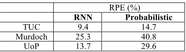
As shown in Table 6, RNN again clearly outperforms the probabilistic approach for all datasets.
Table 6. Prediction Error for Outgoing Users’ Traffic
RPE (%)
RNN Probabilistic
TUC 9.4 14.7
Murdoch 25.3 40.8
[image:7.595.156.438.483.557.2] [image:7.595.203.395.608.662.2]4.4
Outgoing Traffic for System emails
[image:8.595.143.452.257.331.2]This section presents our modeling results for the outgoing system traffic. The range of the total number of outgoing system emails per week for each university’s dataset is presented in Table 7. The vast majority (almost 99%) of these emails have a size smaller than 6 Kbytes. This means that the servers rarely send attachments. Instead, they send short plain messages.
Table 7. Outgoing System Emails’ Numbers and Total Size
Min
#emails #emails Max Gbytes Min Gbytes Max # of weeks
TUC 50480 233653 0.22 2.7 9
LJMU - - - - -
Mur-doch 770 305947 0.007 1.31 52
UoP 2630 8996 0.01 0.05 4
[image:8.595.188.408.453.508.2]As shown in Table 8, RNN once again largely outperforms the probabilistic proach for the TUC and UoP datasets. For the Murdoch dataset the probabilistic ap-proach is shown to have a marginally smaller error, however the results for the proba-bilistic approach refer to 98% of the traffic, excluding the outliers. If the outliers are included, as they are for RNN, the RPE for the probabilistic approach becomes very high for all types of traffic of all datasets.
Table 8. Prediction Error for Outgoing System Traffic
RPE (%)
RNN Probabilistic
TUC 5.3 10.0
Murdoch 23.3 22.6
UoP 4.4 20.4
4.5 Spam Traffic
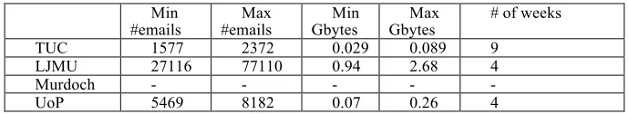
This section focuses on our modeling results for the spam traffic. The range of the total number of outgoing system emails per week for each university’s dataset is presented in Table 9. It should be noted that our dataset from Murdoch University did not contain data for spam traffic.
Table 9. Spam Emails’ Numbers and Total Size
Min
#emails #emails Max Gbytes Min Gbytes Max # of weeks
TUC 1577 2372 0.029 0.089 9
LJMU 27116 77110 0.94 2.68 4
Murdoch - - - - -
[image:8.595.128.473.623.686.2]This is the only case where for one of the datasets (UoP) the probabilistic modeling outperforms RNN, as shown in Table 10 (for the TUC and LJMU datasets again RNN excels). One reason for this different result is that the outliers of the specific spam da-taset make the accurate prediction over the whole dada-taset difficult, whereas the result presented for the probabilistic approach, as explained earlier, focuses on 98% of the traffic, excluding the outliers. The effect of DNS black list settings (which eliminate spam messages at the initial handshake phase, before any data are received, examined and stored), as well as the efficiency of spam detection filters in UoP will be investi-gated further, to gain insight on the reasons behind the high errors of RNN for the UoP dataset.
Table 10. Prediction Error for Spam Traffic
RPE (%)
RNN Probabilistic
TUC 17.1 17.7
LJMU 18.7 36.9
UoP 57.1 25
5
Conclusions
In this work, we model the workload of the email servers of four universities. We ini-tially evaluated various well-known distributions from the relevant literature on work-load characterization, in terms of their fitting accuracy to our data. We found that the accuracy varied, depending on the email traffic category (incoming/outgoing, us-ers/system email or spam) and that even in the cases where a significant accuracy was achieved for the vast majority of the email traffic sizes, there were outliers which could not be accurately predicted.
For this reason, we implemented a Recurrent Neural Network using time series pre-diction, as an alternative method, and we found that it was able to achieve a significantly higher accuracy for all types of email traffic, by treating the datasets as time series. The impressive result with the use of the RNN is that it outperforms the probabilistic ap-proach in terms of accuracy although the RNN models the entirety of the datasets, in-cluding outliers, whereas the probabilistic approach is not used for the outliers, where it fails completely in their modeling.
Acknowledgements
We would like to sincerely thank Mr. Panagiotis Kontogiannis, Head of the Educational Computational Infrastructure at the Technical University of Crete, Mr. Martin Connell, Senior Systems Engineer at LJMU and Mr. Mario Pinelli, Manager of Computer Ser-vices and IT at Murdoch University. Without their help with collecting the datasets this research would not have been possible.
References
1. T. Jackson, R. Dawson, and D. Wilson, "The Cost of Email Interruption," Journal of Systems & Information Technology, vol 5, pp. 81-92, 2001.
2.T. Takemura, and H. Ebara, "Spam Mail Reduces Economic Effects," in Proc. of the 2nd IEEE International Conference on the Digital Society, 2008.
3. A. Kashyap et al., "Internet Security Threat Report 2014,"[Online]: http://www.symantec.com/content/en/us/enterprise/other_resources/b-istr_main_report_v19_21291018.en-us.pdf
4. L.H. Gomez et al, "Workload models of spam and legitimate e-mails," Performance Evaluation , Vol. 64, No. 7-8, 2007.
5. L.Bertolotti and M.C. Calzarossa, "Workload Characterization of Email Servers," in Proceedings of SPECTS, 2000.
6. S. Shah and B.D. Noble , "A study of e-mail patterns," Software - Practice and Experience, Vol. 37, No. 14, 2007.
7. V. Paxson, "Empirically-Derived Analytic Models of wide-area TCP connections," IEEE/ACM Transactions on Networking, Vol. 2, No. 4, 1994.
8.T. W. Anderson and D. A. Darling, "Asymptotic Theory of Certain "Goodness of Fit" Criteria Based on Stochastic Processes", Annals of Mathematical Statistics, Vol. 23, No. 2, 1952. 9. A.M. Law, W.D. Kelton, Simulation Modeling & Analysis, 2nd ed., McGraw-Hill, 1991. 10. F. J. Massey, “The Kolmogorov-Smirnov Test for Goodness of Fit”,Journal of the American Statistical Association, Vol. 46, No. 253, 1951.
11. S.Kullback and R.A. Leibler, "On Information and Sufficiency," The Annals of Mathematical Statistics, Vol. 22, No. 1, 1951.
12. L. I. Lanfranchi and B.K. Bing, "MPEG-4 Bandwidth Prediction for Broadband Cable Networks," IEEE Transactions on Broadcasting, Vo. 54, No. 4, 2008.
13. S. Boukoros, A. Kalampogia and P. Koutsakis, "A New Highly Accurate Workload Model for Campus Email Traffic," in Proceedings of the International Conference on Computing, Networking and Communications (ICNC) 2016.
14. N. Navaroli, C. DuBois and P. Smyth, “Statistical Models for Exploring Individual Email Communication Behavior”, in Proc. of the Asian Conference on Machine Learning 2012. 15. M. Hüsken and P. Stagge, “Recurrent Neural Networks for Time Series Classi cation”, Neurocomputing, Vol 50 No. C, 2013.
16. M. Längkvist, L. Karlsson and A. Loutfi, “A review of unsupervised feature learning and deep learning for time-series modeling”, Pattern Recognition Letters, Vol. 42, No. 1, 2014. 17. A. M. Rather, A. Agarwal and V. Sastry, “Recurrent neural network and a hybrid model for prediction of stock returns”, Expert Systems with Applications, Vol. 42, No. 6, 2015.