Numerical simulation of double diffusive mixed convection and entropy generation in a lid driven trapezoidal enclosure with a heat source

warwick.ac.uk/lib-publications

Ababaei, Ahmad, Abbaszadeh, Mahmoud, Arefmanesh, Ali and Chamkha, Ali J. (2018) Numerical simulation of double-diffusive mixed convection and entropy generation in a lid-driven trapezoidal enclosure with a heat source. Numerical Heat Transfer, Part A:

Applications, 73 (10). pp. 702-720. doi:10.1080/10407782.2018.1459139 Permanent WRAP URL:

http://wrap.warwick.ac.uk/103623 Copyright and reuse:

The Warwick Research Archive Portal (WRAP) makes this work by researchers of the University of Warwick available open access under the following conditions. Copyright © and all moral rights to the version of the paper presented here belong to the individual author(s) and/or other copyright owners. To the extent reasonable and practicable the material made available in WRAP has been checked for eligibility before being made available.

Copies of full items can be used for personal research or study, educational, or not-for profit purposes without prior permission or charge. Provided that the authors, title and full bibliographic details are credited, a hyperlink and/or URL is given for the original metadata page and the content is not changed in any way.

Publisher’s statement:

“This is an Accepted Manuscript of an article published by Taylor & Francis in Numerical Heat Transfer, Part A: Applications on 31/05/2018 available

online: https://doi.org/10.1080/10407782.2018.1459139 A note on versions:

The version presented here may differ from the published version or, version of record, if you wish to cite this item you are advised to consult the publisher’s version. Please see the ‘permanent WRAP URL’ above for details on accessing the published version and note that access may require a subscription.

1

Numerical simulation of double-diffusive mixed convection and entropy

generation in a lid-driven trapezoidal enclosure with a heat source

Ahmad Ababaeia_{, Mahmoud Abbaszadeh}b,*_{, Ali Arefmanesh}a_{, Ali J. Chamkha}c,d

a_{Department of Mechanical Engineering, University of Kashan, Kashan, Iran (Postal Code:}

8731753153)

b_{School of Engineering, University of Warwick, Coventry CV4 7AL, United Kingdom}

c _{Mechanical Engineering Department, Prince Sultan Endowment for Energy and Environment,}

Prince Mohammad Bin Fahd University, Al-Khobar 31952, Saudi Arabia

d _{RAK Research and Innovation Center, American University of Ras Al Khaimah, P.O. Box}

10021, Ras Al Khaimah, United Arab Emirates

Abstract

In this study, entropy generation of double-diffusive mixed convection is investigated inside a

right-angled trapezoidal cavity with a partially heated and salted bottom wall. Similar to the

approach that assigns color to streamlines, a new coloring scheme is employed to visualize

heatlines and masslines in a more meaningful manner. In addition, various consequential

parameters, namely the Lewis and Richardson numbers, the buoyancy ratio, the direction of lid

movement, and the heat source location, have been analyzed. According to the results, as the

Lewis number increases, the average Nusselt number declines, while the total entropy generation

augments. Furthermore, for Le = 0.1, the conduction mass transfer dominates the mass transfer

field; hence, the masslines are virtually perpendicular to the isoconcentration lines.

Keywords:

mass transfer; Entropy generation.

*_{Corresponding author}

2

Nomenclature

Be Bejan number

Br buoyancy ratio

c species concentration (kg m-3₎

C dimensionless species concentration

D mass diffusivity (m2 s-1)

Gr Grashof number

g gravitational acceleration (m s-2₎

H dimensionless heatfunction

k thermal conductivity (W m-1 _K-1₎

L enclosure length (m)

Lh heat source distance from origin (m)

Le Lewis number

M dimensionless massfunction

n unit normal vector

Nu Nusselt number

p pressure (N m-2)

P dimensionless pressure

Pr Prandtl number

R gas constant (= 8.314 J mol-1 K-1)

Re Reynolds number

Ri Richardson number

s& volumetric rate of entropy generation (W m-3 K-1)

S& dimensionless volumetric rate of entropy generation

S& dimensionless overall rate of entropy generation

Sh Sherwood number

T temperature (K)

3













Greek symbols

α thermal diffusivity (m2 s-1)

βc coefficient of solutal expansion (m3 kg-1) βT coefficient of thermal expansion (K-1)

γ Angle between inclined and bottom wall

θ dimensionless temperature

μ dynamic viscosity (kg m-1 s-1) ν kinematic viscosity (m2 s-1)

ρ density (kg m-3)

i



Ψ dimensionless streamfunction

Ω computational domain

Subscripts

0 reference state

av average or mean

c cold

h hot or high

l low

Superscripts

4

1.

Introduction

As far as the world’s fossil fuel resources are limited, considerable efforts should be directed

into designing devices and processes in engineering systems. Furthermore, in order to attain

multi-faceted targets of an engineering system, a creative, iterative, and open-ended process

which results in effective thermal and fluid system designing, is required. To satisfy such a need,

the Second Law of Thermodynamics should be considered in analyzing a thermal fluid system to

promote its energy efficiency. Moreover, the criterion to assess for energy efficiency of

engineering devices is entropy generation which plays a significant role in clarifying the

maximum theoretical limits of energy efficiency. It is worth mentioning that the thermal, friction,

and other thermodynamic irreversibilities, which are responsible for inefficiencies in an

engineering thermal fluid system, are taken into account in formulating entropy generation.

Numerous studies were dedicated to scrutinize the entropy generation and convection heat

transfer in enclosures over the past few years [1-11]. Baytas [12] conducted a numerical

simulation to study entropy generation and natural convection heat transfer in an inclined square

cavity. He observed that in low Rayleigh numbers that the effects of heat transfer irreversibility

are more than fluid friction irreversibility. Natural convection heat transfer and entropy

generation in a square enclosure is numerically investigated by Mahmud and Fraser [13]. Based

on their results, the entropy generation in the center of the enclosure is lower in magnitude

compared to near the cavity walls. In another numerical investigation, Ovando-Chacon et al. [14]

examined entropy generation due to mixed convection heat transfer in a square cavity. They

observed that the high entropy generation due to fluid friction irreversibility occurs near the

vertical moving walls; and the minimum and maximum entropy generation due to heat transfer

irreversibility takes place on the middle of the cavity walls and in the zones with large

temperature gradients, respectively. Moreover, they demonstrated that when the Richardson

number increases, the heat transfer irreversibility near the boundaries of the cavity increases.

Khorasanizadeh et al. [15] utilized the finite volume method and the SIMPLER algorithm to

explore mixed convection and entropy generation in a lid-driven square cavity. Based upon their

results, when the Reynolds number increases, both terms of entropy generation augment; and as

the Rayleigh number increases, the heat transfer term of entropy generation increases and

5

entropy generation is for low Rayleigh and high Reynolds numbers, and the minimum entropy

generation appertains to low Rayleigh and low Reynolds numbers. Very recently, Nayak et al.

[16] conducted a numerical investigation to explore mixed convection heat transfer and entropy

generation in a lid-driven square enclosure. The results have shown that the entropy is generated

mainly because of heat transfer irreversibility. They also concluded that the Bejan number

increases as the Reynolds number increases at a constant Grashof number, but it decreases with

increase of the Grashof number when the Reynolds number is constant. Mixed convective heat

transfer of nanofluid and its entropy generation in a trapezoidal cavity is examined by Aghaei et

al. [17]. They observed that in all of considered cases, the entropy generation due to fluid friction

is negligible and entropy virtually generated due to heat transfer. They also showed that in

Reynolds number of 1000, moving direction of the lid does not have profound effects on the total

entropy generation and the average Nusselt number, but in Reynolds number of 30 this behavior

is completely reversed.

When the buoyancy forces take place as a result of temperature and concentration gradients,

the concept of double-diffusive natural convection appears. In other word, in order to calculate

the density of a fluid, the effects of the temperature gradients and concentration gradients should

be taken into account simultaneously. Double-diffusive natural convection has been encountered

in different ranges of natural systems such as atmosphere, ocean circulation, asthenosphere

movement within crust, pollution transportation in air, astrophysics, geology, biology, chemical

processes, etc. The debate surrounding double-diffusive convection has witnessed many

controversies in the last three decades [18-24]. As early as 1987, Trevisan and Bejan [25]

numerically and analytically examined natural convection heat transfer due to the buoyancy

effects of both temperature and concentration in a rectangular slot subjecting to uniform heat and

mass fluxes. Double-diffusive natural convection of moist air flowing inside a square cavity with

heat and mass diffusive walls is investigated by Costa [26] using the SIMPLER algorithm based

on finite volume method. They obtained that buoyancy ratio has a great impact on both the

temperature and concentration fields, parameters of both heat and mass transfer fields as well as

the routes tracked by the heat and mass streams. Al-Amiri et al. [27] conducted a numerical

simulation to study mixed convection heat transfer in a lid-driven square enclosure under the

buoyancy effects of both thermal as well as solutal diffusion. Based on their results,

6

numbers due to the moving lid. Moreover, they observed that Lewis number has not far-reaching

effect on the isotherms and streamlines in small Richardson numbers. In another numerical

investigation, Hasanuzzaman et al. [28] analyzed double-diffusive mixed convection in a right

triangular enclosure occupied with air. They showed that as the Lewis number increases, heat

transfer decreases for all studied parameters. They also demonstrated that when the Lewis

number augments, the Sherwood number increases almost linearly; also, higher Sherwood

numbers appertain to higher values of Richardson numbers. Oueslati et al. [29] carried out a

numerical study to explore entropy generation of double-diffusive natural convection inside a

rectangular enclosure with partial, vertical, thermal and solutal sources. They observed that by

increasing the Lewis number, the heat and mass transfer rates significantly increases. They also

concluded that the entropy generation is low within the enclosure with the exception of the

vicinity of the active vertical walls, especially in the zones where there are high velocity

gradients. Qin et al. [30] numerically investigated double-diffusive convection of a binary mixed

fluid in a rectangular enclosure with horizontal temperature and concentration gradients. Their

results showed that the Sherwood number increases with the Lewis number. Very recently, Arbin

et al. [31] numerically studied double-diffusive natural convection in an open top square cavity

via the heatlines approach. According to their findings, higher values of Lewis number will

decrease the heat transfer rates, but will enhance the mass transfer rates. Teamah et al. [32]

numerically investigated the double-diffusive natural convection in the presence of magnetic

field inside a trapezoidal cavity. The results showed that heat and mass transfer rates decline

when the Hartmann number increases.

In order to gain a better physical insight about heat and mass transfer in enclosures, the

heatlines and masslines visualization techniques have been proposed as innovative approaches

which pave the way. In order to visualize how the energy flows through the convective heat

transfer fields, heatlines were presented and used for the first time by Kimura and Bejan [33].

Subsequently, masslines were put forward by Trevisan and Bejan [25] in order to visualize

convective mass transfer fields. Then, Costa [34] presented a thorough survey on the use of

heatlines and masslines. As a glance at aforementioned literature, and even the new studies

where heatlines and masslines visualization techniques are used [35-37], it is incontrovertibility

axiomatic that the coloring scheme is not applied in most of the studies. Moreover, in only a few

7

meaningful. Therefore, in this study, heatlines, masslines, and streamlines are colored in a way

that there is a quite clear-cut distinction between the zones where the momentum, heat, and mass

transfer are higher and those where the momentum, heat, and mass transfer are lower.

As evidenced by immense, well-documented, and proliferation literature pertaining to

double-diffusive convection, it is crystal clear that there has been a little focus on entropy generation of

double-diffusive mixed convection inside a trapezoidal cavity and an in-depth analysis about it

remains to be addressed. Also, the colored heatlines and masslines technique have never been

used in any of these studies. Hence, in this study, double-diffusive mixed convection heat

transfer and entropy generation in a trapezoidal enclosure is examined. The set of equations

associated with this problem are numerically solved by employing the well-known SIMPLER

algorithm. The convective heat and mass transfer fields are depicted using colored heatlines and

masslines. The effects of different parameters such as the Lewis number, buoyancy ratio,

Richardson number, direction of lid movement and the heat source location are discussed and

assessed, and the implications of using these parameters on heat and mass transfer as well as

entropy generation are investigated.

2.

Physical model and formulation

2.1.Physical model and governing equations

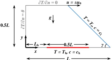
The shape of the cavity is displayed in Fig. 1. It has a height of 0.5L and its lower wall has

length L. The enclosure’s inclined wall is kept at low temperature and low concentration Tc and cl, respectively. Moreover, the partially heated and salted lower wall is maintained at constant

temperature and concentration Th and ch, respectively. The heat and mass sources are coincident.

The remaining walls of the cavity are insulated and impermeable. The top wall moves from right

to left and vice versa with a constant speed u0. The incompressible fluid is presumed to be

Newtonian. All of the thermo-physical properties of the fluid are considered to be constant

except for the density variations in the buoyancy terms where the Boussinesq approximation is

applied as follows:









0 1 T T Tc c c cl

8

where₀is the fluid density at the reference temperature and concentration of T₀ 





and c₀ 

















thermal and solutal expansion coefficients, respectively.

The balance equations of mass, momentum, energy, and species concentration for the steady,

laminar, two-dimensional mixed convection fluid flow and heat and mass transfer are as follows:

0

u v

x y

 _ _

  , (2)

2 2 2 2

1

u u p u u

u v

x y  x  x y

 

 _  _{ }  _  _ 

 

   _  _, (3)









v v p v v

u v g T T c c

x y  y  x y  

 

 _  _{ }  _  _  _{     }

   

   _  _ , (4)

2 2 2 2

T T T T

u v

x y  x y

   _  _  _     _  _ , and (5) 2 2 2 2

c c c c

u v D

x y x y

 

   

  _  _

  _  _, (6)

where u and vare the velocity components in the x and y directions, respectively.  and  are

the fluid density and the kinematic viscosity, respectively. Moreover, T, p, c, g, , and D are the

temperature, the pressure, the concentration, the gravitational acceleration, the thermal

diffusivity, and the mass diffusivity, respectively.

The volumetric rate of generated entropy [39], assuming that the fluid behaves as a binary

perfect gas mixture [40], can be calculated as follows:

2 2 2

2 2 2 0 0 2 2 0 0 2 ,

k T T u v u v

s

T x y T x y y x

RD c c RD T c T c

c x y T x x y y

9

where R is the gas constant which is equal to 8.314 J/mol K.

The set of Eqs. (2)–(6) can be changed to their dimensionless forms by replacing the main

parameters with their corresponding dimensionless variables that are given below:



   

  

0 0

, ,

, x y , , u v , p , T T , c c

X Y U V P C

L u u  T c

 

    

  , (8)

where  T T_hT_c and   c c_h c_l. Using the foregoing dimensionless variables, the

dimensionless form of the governing equations is written as:

0

U V

X Y

 _ _

  , (9)

2 2

2 2

1 Re

U U P U V

U V

X Y X X Y

 

 _  _{ } _  _ 

 

   _  _, (10)





U U P U V

U V C

X Y X X Y 

 

 _  _{ }  _  _  _{ }

 

   _  _ , (11)

2 2

2 2

1 RePr

U V

X Y X Y

       _  _  _      _  _ , and (12) 2 2 2 2 1 RePrLe

C C C C

U V

X Y X Y

 

   

  _  _

  _  _, (13)

where the Reynolds, Prandtl, Lewis, Grashof and Richardson numbers, and the buoyancy ratio

are defined, respectively, as

3 0

2 2

Gr

Re , Pr , Le , Gr , Ri , Br

Re

c T

T

u L g TL c

D T                  (14)

The Prandtl and Grashof numbers, which are considered to be constant in this study, are equal

to Pr0.71 and Gr104, respectively.

10

2 2 2 2 2

2 2 0

1 2

2 2

2 3 ,

2

L T C U V U V

S s

k T X Y X Y Y X

C C C C

X Y X X Y Y

 _       _{    }  _{    } _{  }   _ _{ } __{ }   _ _ __ _ _ _ _              _{   }  _{       }  _{ } _{ }  _{   } _{ }                     & _& (15)

where ₁,₂and₃ ,which denote the irreversibility distribution ratios, are defined as follows:

2 2

0 0

1 2 0 3 0

0

, ,

T u RD c RD c

T T

k T kc T k T



  _ _   _  _   _  _

      

  (16)

It is to be noted that these irreversibility distribution ratios are assumed constant and equal to

4 1 10

 _ 

,₁ 0.5and₁102 [29, 40, 41].

The corresponding non-dimensional boundary conditions for Eqs. (9)–(13) are as follows:

0

U  V _{, and}   C 1 on the sources,

0

U  V ,and  C 0 _{at the inclined wall,}

1, 0

U   V  ,and C 0

n n



 _ _

  at the top wall,

0 C U V n n       

  along the remaining walls.

(17)

The overall rate of entropy produced by the irreversibilities can be calculated by integrating

the volumetric rate of irreversibilities over the entire domain as follows:

S S d







_

& &

(18)

The average Nusselt and Sherwood numbers along the heat and mass source on the bottom

wall are evaluated from the following equations:

* h * h 0.5 av 0 1 Nu 0.5 L L Y dX Y       



11 where L*_h L_h L.

2.2.Visualization Method

In this study, the integration method [42] is employed to visualize streamlines, heatlines, and

masslines. Moreover, a new coloring approach is also used for the purpose of illustrating

heatlines and masslines in a more meaningful manner. This approach is going to be discussed

later in this section.

Initially, a bird’s-eye view of the entire flow field and its main characteristics are

demonstrated by means of the streamfunction, which is obtained from the conservation of mass

equation. The streamfunction values can be calculated from:









, , 0 X Y

X

X Y X UdY

   

_

where   ₀

 









0 , 0 0

Y

X _ V X

     .

The conservation of energy equation can be rearranged and, similar to the streamfunction, the

heatfunction can be defined as:

* _, H U Y X     _{ } 

  and

* H V X Y        

  , (22)

where * 1 Re Pr. Obviously, the heatfunction is able to satisfy the conservation of energy

equation. It represents the local strength of the convective heat transfer, which is composed of

the advective heat fluxes









by integrating Eq. (22) as follows:





 

* 0,0

, 0 0, 0 X ,

H X H V dX

Y         _  _   











, , 0 X Y

X

H X Y H X U dY

X         _  _   

12 where H₀ H

 

A similar conclusion can be drawn after the conservation of species concentration equation is

rearranged:

*

,

M C

UC D

Y X

 _{ } 

  and

*

M C

V C D

X Y

 

  

  , (24)

where D* 1 Re PrLe. The massfunction values, which consist of advective and conductive

mass fluxes, is calculated by integrating (24) as follows:





 

* 0,0

, 0 0, 0 X C ,

M X M D VC dX

Y



 

  _  _



 



and

(25)









* ,0

, , 0 X Y ,

X

C

M X Y M X UC D dY

X



 

  _  _



 



where M₀ M

 

The mentioned coloring approach presents the heatlines and masslines in a way that is both

meaningful and easier to interpret. This is analogous to the coloring of streamlines when they are

colored by absolute values of velocity (i.e. u2v2 ). Thus, absolute convective values of

heatlines and masslines are applied as coloring on the lines. In other words, streamlines,

heatlines, and masslines are colored in each point with values of U2V 2 ,



 



H X H Y

     , and



 



coloration of heatlines and masslines shows the local intensity of energy or mass transfer rate in

the heat or mass transfer field. Hence, it becomes easier to appreciate and analyze these fields.

3.

Numerical implementation

By using the finite volume method [43], a FORTRAN code is developed in order to solve the

13

handle the coupling between the pressure and velocities. The diffusive and advective terms in

Eqs. (10)–(13) are discretized by employing the power-law differencing scheme, and the

corresponding set of discretized equations are solved using a TDMA line-by-line solver.

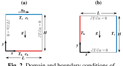
3.1.Benchmarking of the code

The correct modeling of the code is verified by developing a similar code to simulate the

existing results of other studies. The geometries as well as the boundary conditions of the

considered test cases are illustrated in Fig. 2. Comparisons between the heat transfer, the fluid

friction irreversibilities, the total rate of entropy generation, and the local Bejan number of the

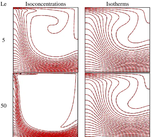
present study code with those of Ilis et al. [45] are shown in Fig. 3 for Pr = 0.7 in Ra = 105. Moreover, Fig. 4 shows comparisons between the isotherms and the isoconcentration lines in the

square enclosure using the developed code with the results of Al-Amiri et al. [27]. The results in

this figure are for Pr = 1, Ri = 0.01, Re = 100, Br = 1 and Le = 5 and 50. Figs. 3 and 4 exhibit a

sufficiently good agreement between the simulated results of the present code and those of

Al-Amiri et al. [27] and Ilis et al. [45], thereby guaranteeing the accuracy of the findings acquired

by the present study.

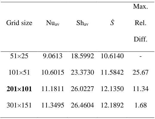
3.2.Finding an independent grid

To find a proper grid for the numerical simulations, a test of grid independency is conducted

for the mixed convection flow at Ri = 100, Le = 10, Br = -10, and γ = 45°. The obtained average

Nusselt number and the total entropy generation for different girds are presented in Table 1. As

evidenced by this table, when the grid 201×101 is replaced with the grid 301×151, the maximum

relative difference between the two grid systems becomes 1.68%, which is clearly a negligible

change. Therefore, the grid system having 201×101 nodes is a proper grid for simulations and it

is applied to the subsequent numerical calculation. All of the following results are obtained

employing this grid.

4.

Results and discussion

The entropy generation of double-diffusive mixed convection is examined in a right-angled

trapezoidal cavity that is partially heated and salted. The effects of different parameters such as

14

and the heat source location on the flow and temperature fields are studied. The study is

conducted for 0.01 < Ri < 100, -10 < Br < 10, 0.1 < Le < 10, Pr = 0.7, Gr = 104, and γ = 45° and 60°.

4.1. Isotherms, isoconcentration lines, streamlines, heatlines, masslines, and constant entropy

generation lines

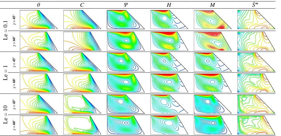
Fig. 5 displays the isotherms, the isoconcentration lines, the streamlines, the heatlines, the

masslines, and the constant entropy generation lines for Le = 10, Br = 1, Ri = 0.1 and 10, γ = 45°

and 60°, and for the two directions of the lid movement. As can be seen from this figure, when

the lid moves toward the right side, the clockwise vortex draws the isotherm and the

isoconcentration lines from the cold wall toward the heat source, and accumulates them on the

heat source. Furthermore, the isotherm and isoconcentration lines are less compressed on the

heat source for  60o compared to when  45o due to the fact that for  60o, the distance

between the cold wall and heat source is more compared to when  45o. Moreover, the

accumulation of the isotherm and the isoconcentration lines on the hot and the cold boundaries

diminish for Ri = 10 compared to when Ri = 0.1 due to the enhanced natural convection strength.

A close scrutiny of the streamlines, the heatlines, and the masslines reveals that the velocities

have the maximum values near the moving wall. Moreover, the heatlines and the masslines

emerge vertically from the heat source and after taking effect from the central vortex,

perpendicularly reach to the cold wall. Above the right section of the heat source and upper parts

of the cold wall, the heatlines and the masslines have the maximum density implying the

maximum rates of heat and mass transfer in these areas, respectively. According to the lines of

constant generated entropy, the maximum amount of local generated entropy is seen over the

right side of the heat source and upper parts of the cold wall, and the minimum entropy

generation takes place on the left bottom corner of the enclosure. Furthermore, when the lid

moves toward the left side, the counterclockwise vortex stretches the isotherm and the

isoconcentration lines from the heat source toward the cold wall. In this case, a secondary

clockwise vortex develops in the right corner of the enclosure which becomes larger with

increasing the Richardson number. This vortex alters the layout of the heatlines and the

15

to the lines of constant generated entropy, the generated entropy in the central part of the heat

source decreases in this case.

Fig. 6 illustrates the isotherms, the isoconcentration lines, the streamlines, the heatlines, the

masslines, and the constant entropy generation lines for Ri = 1, Br = 4, and γ = 45° and 60° and

for different Lewis numbers. As it is observed from the isotherms and the heatlines, variations of

the Lewis number does not have a considerable impact on these lines due to the fact that the

Lewis number does not affect the energy equation directly. Regarding the isoconcentration lines,

increasing the Lewis number compresses the isoconcentration lines, on the high and low

concentration walls; while, a region with an average concentration is extended in the central part

of the enclosure. Furthermore, high values of the Lewis number signify less mass diffusivity.

When the mass diffusivity decreases, the solutal boundary layer becomes thinner and, therefore,

the concentration gradient on both high and low salted walls increases resulting in mass transfer

enhancement. It is noteworthy that for Le = 1, the diffusion characteristics of heat and mass

transfer are identical and as results, the isotherm and isoconcentration lines, as well as the

heatlines and the masslines are coincident. Considering the color of streamlines, as the Lewis

number increases, the strength of the flow declines, but the structure of the streamlines is

maintained. Regarding the masslines, for Le = 0.1, the conduction mass transfer dominates the

mass transfer field and so, the masslines are virtually perpendicular to the isoconcentration lines;

while by increasing the Lewis number, the masslines are more affected by the primary vortex

due to the fact that the conductive mass flux decreases when the Lewis number augments. The

constant generated entropy lines show that the entropy generation increases with the Lewis

number.

The isotherms, the isoconcentration lines, the streamlines, the heatlines, the masslines, and the

constant entropy generation lines for Ri = 100, Le = 0.1, γ = 45° and different buoyancy ratios

and heat source locations are shown in Fig. 7. Regarding the isotherms, whenL_h 0, the

isotherms are drawn from the hot surface toward the cold wall for Br 10. This behavior is

completely reversed for Br 10 due to the change of the rotating direction of primary vortex

from counterclockwise for Br 10 to clockwise for Br 10 . Moreover, for Br 10, the

downward solutal buoyancy force overwhelmingly dominates the upward thermal buoyancy

16

effect on flow field, the temperature gradient on the heat source is less than that of the other

cases. Regarding the isoconcentration lines, by increasing the buoyancy ratio from -10 to 10, the

concentration gradient on the mass source increases. As far as the heatlines and masslines, the

heatlines are under the influence of the counterclockwise and clockwise circulations for

Br 10 andBr 10 , respectively. Furthermore, the primary vortex for Br0 does not affect

the masslines; and the masslines are perpendicular to the isoconcentration lines. This behavior

reveals that the conductive mass transfer regime is dominant for Le = 0.1. By considering the

constant entropy generation lines, the maximum irreversibility takes place in the right edge of

heat source and the upper part of the cold wall. Moreover, forL_h 0.25, as the heat source

approaches the cold wall, both of the temperature and concentration gradients increase.

According to the constant generated entropy lines, the local generated entropy is maximum at the

right side of the heat source. Furthermore, for L_h 0.5, as the heat source approaches toward the

cold wall, strong temperature and concentration gradients develop in the right corner of the

enclosure. ForBr 10, one primary counterclockwise vortex, accompanied with two secondary

clockwise vortices, is formed within the enclosure. ForBr0, there is just one clockwise vortex,

but forBr 10 , one counterclockwise vortex in the left bottom corner of the enclosure is created.

Moreover, the heatlines directly reach to the cold wall due to the counterclockwise circulation

for Br 10; whereas for Br 10 , the heatlines initially move toward the center of the enclosure

and then, reach to the cold wall. It is worth mentioning that the buoyancy ratio does not affect the

masslines significantly; and the maximum entropy generation occurs in the right corner of the

enclosure.

4.2.Temperature, concentration and velocity profiles

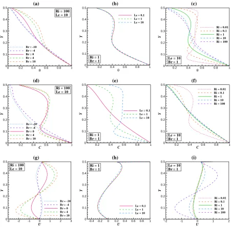
Fig. 8 displays the variations of the dimensionless temperature, concentration, and velocity

along the vertical centerline of the enclosure for γ = 45° and for different buoyancy ratios and

Lewis and the Richardson numbers. As can be observed from this figure, by increasing the

buoyancy ratio, the temperature in the upper half of the enclosure augments. Moreover, as the

Richardson number decreases, the temperature gradients on the top and bottom walls increase

and a region with an average temperature develops in the center of the enclosure. Moreover, for

Br0, the concentration decreases linearly with the height, but for Br0, the concentration in

17

height. Also, as the Lewis number increases due to diminishing effects of mass diffusion, the

concentration gradient on the top and bottom wall augments and a region with an average

concentration expands in the center of the enclosure. It should be noted that the variations of the

Lewis number does not have significant effect on the velocity profile, and with decreasing the

Richardson number, the velocity gradient increases.

4.3.Mean Nusselt and Sherwood numbers, and overall entropy generation

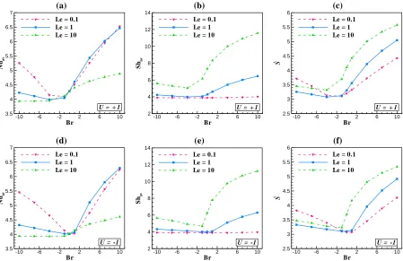
Fig. 9 shows variations of the mean Nusselt and Sherwood numbers and the overall generated

entropy with the buoyancy ratio for Ri = 10 and γ = 45° and for different Lewis numbers and two

directions of the lid movement. In Figs. 9 a and b, the average Nusselt number decreases when

the Lewis number increases. On the other hand, for Le = 0.1 and 1, with augmentation of the

buoyancy ratio, the average Nusselt number initially decreases and then increases, because when

Br 0, the buoyancy forces intensify. Furthermore, whenBr0, the mean Nusselt number

is larger when the lid moves toward the left compared to when it moves toward the right. This

behavior is reversed forBr0. As it is observed from Figs. 9 c and d, the average Sherwood

number decreases as the Lewis number increases. Moreover, with augmentation of the buoyancy

ratio, the average Sherwood number initially decreases slightly and then, increases significantly.

Similar to the average Nusselt number, for Br0, the average Sherwood number is high as the

lid moves toward the left compared to when it moves toward the right; whereas, this behavior is

reversed for Br0. According to Figs. 9 e and f, with increasing the Lewis number, the entropy

generation augments for Br0. Moreover the entropy generation is higher when the lid moves

toward the right compared to when it moves toward the left; while, for Br0, the minimum

entropy generation belongs to Le = 1 and after that to Le = 10 and 0.1; and when the lid moves

toward the right side, the entropy generation is less than when the lid moves toward the left side.

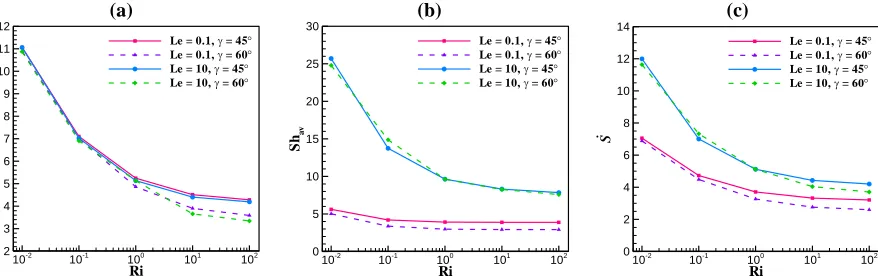
Fig. 10 illustrates how the mean Nusselt and Sherwood numbers, and the overall generated

entropy change with the Richardson number for Br = 1, Le = 0.1 and 10, and γ = 45° and 60°.

Generally, with increasing the Richardson number and decreasing the temperature, the

concentration, and the velocity gradients (see Figs. 8 c, f, and i), the mean Nusselt and Sherwood

numbers, and the overall generated entropy decrease. Furthermore, the mean Nusselt and

18

because by decreasing  , all the gradients increase. Regarding Figs. 10 a and c, when the Lewis

number increases, the mean Nusselt number diminishes, while the entropy generation augments.

According to Fig. 10 b, for Le = 0.1 when the conduction mass transfer is dominant (see Fig. 6),

changing the Richardson number does not have a significant effect on the average Sherwood

number.

Variations of the average Nusselt and Sherwood numbers as well as the total entropy

generation with the buoyancy ratio are depicted in Fig. 11 for Le = 10, γ = 45° and in different

Richardson numbers. According to this figure, by decreasing the Richardson number, the mean

Nusselt and Sherwood numbers, and the total generated entropy augment. Also, by reducing the

Richardson number and diminishing the buoyancy term in Y-momentum equation, the impact of

buoyancy ratio on the mean Nusselt and Sherwood numbers as well as the total entropy

generation declines. Moreover, for Le = 10, when the buoyancy ratio increases, the mean Nusselt

and Sherwood numbers, and the overall generated entropy monotonically increase for Ri1; while forRi0.1, They initially decrease and then augment.

In Fig. 12, variations of the mean Nusselt and Sherwood numbers and the total entropy

generation in terms of the Richardson number are displayed for Br = 1, Le = 0.1, γ = 45° and for

different locations of the heat source on bottom wall. As can be seen from this figure, for a

constant buoyancy ratio, as the Richardson number increases, the average Nusselt and Sherwood

numbers, and the total entropy generation decline. Furthermore, asL*h 0.5, the mean Nusselt

and Sherwood numbers, and the total generated entropy drastically increase compared to the

other cases. Moreover, changing the Richardson number does not have a meaningful influence

on the average Sherwood number for Le = 0.1.

5.

Conclusion

In this study, the finite volume method (FVM) is employed in order to study the entropy

generation of double-diffusive mixed convection in a right-angled trapezoidal enclosure filled

with a binary perfect gas mixture. Also, the convective heat and mass transfer fields are depicted

using colored heatlines and masslines, which both proved to be useful tools for interpretation as

well as analysis. The effects of the consequential parameters such as the Lewis number, the

19

location on the heat and mass transfer as well as the entropy generation are examined. Based on

the results, the following observations are made:

 The mean Nusselt and Sherwood numbers, and the overall generated entropy for  45o

are more than those for  60o due to the fact that the gradient of the dependent

variables increases as  is reduced.

 ForBr0, when the lid moves toward the left, the mean Nusselt and Sherwood

numbers, and the overall generated entropy are more compared to the case where the lid

moves toward the right; while, this behavior is reversed forBr0.

 As the heat source approaches the cold wall, the mean Nusselt and Sherwood numbers,

and the overall generated entropy increase, especially for L*h 0.5 they increase

dramatically.

 With the increasing of the Lewis number, the mean Nusselt number decreases, while the

entropy generation augments.

 Variation of the Lewis number does not have a considerable impact on the isotherms and

the heatlines, but increasing the Lewis number compresses the solutal boundary layer

and, therefore, the concentration gradient on both high and low salted walls increases,

resulting in mass transfer augmentation.

 For Le = 0.1, the conduction mass transfer dominates the mass transfer field and so, the

masslines are virtually perpendicular to the isoconcentration lines. Moreover, the

Richardson number does not have a meaningful influence on the average Sherwood

number for Le = 0.1.

 With decreasing the Richardson number and the buoyancy term for the Y-momentum

equation, the impact of the buoyancy ratio on the mean Nusselt and Sherwood numbers

as well as the total entropy generation decline. Moreover, for Le = 10, with increasing

the buoyancy ratio, the mean Nusselt and Sherwood numbers, and the overall generated

20

6.

References

[1] A. Bejan, Entropy generation minimization: the method of thermodynamic optimization

of finite-size systems and finite-time processes: CRC press, 1995.

[2] S. Mahmud and A. S. Islam, Laminar free convection and entropy generation inside an

inclined wavy enclosure, International journal of thermal sciences, vol. 42, pp.

1003-1012, 2003.

[3] C. Balaji, M. Hölling, and H. Herwig, Entropy generation minimization in turbulent

mixed convection flows, International Communications in Heat and Mass Transfer, vol.

34, pp. 544-552, 2007.

[4] I. Zahmatkesh, On the importance of thermal boundary conditions in heat transfer and

entropy generation for natural convection inside a porous enclosure, International

Journal of Thermal Sciences, vol. 47, pp. 339-346, 2008.

[5] A. H. Mahmoudi, M. Shahi, and F. Talebi, Entropy generation due to natural convection

in a partially open cavity with a thin heat source subjected to a nanofluid, Numerical Heat

Transfer, Part A: Applications, vol. 61, pp. 283-305, 2012.

[6] M. Esmaeilpour and M. Abdollahzadeh, Free convection and entropy generation of

nanofluid inside an enclosure with different patterns of vertical wavy walls, International

Journal of Thermal Sciences, vol. 52, pp. 127-136, 2012.

[7] A. Bejan, Convection heat transfer: John wiley & sons, 2013.

[8] A. Arefmanesh, A. Aghaei, and H. Ehteram, Mixed convection heat transfer in a CuO–

water filled trapezoidal enclosure, effects of various constant and variable properties of

the nanofluid, Applied Mathematical Modelling, vol. 40, pp. 815-831, 2016.

[9] M. Abbaszadeh, A. Ababaei, A. A. Abbasian Arani, and A. A. Sharifabadi, MHD forced

convection and entropy generation of CuO-water nanofluid in a microchannel

considering slip velocity and temperature jump, Journal of the Brazilian Society of

Mechanical Sciences and Engineering, vol. 3, pp. 775-790, 2016.

[10] A. Ababaei, M. Abbaszadeh, and A. A. Abbasian Arani, Determining the Optimum

Arrangement of Micromixers in a Microchannel Filled with CuO-Water Nanofluid via

21

[11] A. Ababaei, A. A. Abbasian Arani, and A. Aghaei, Numerical Investigation of Forced

Convection of Nanofluid Flow in Microchannels: Effect of Adding Micromixer, Journal

of Applied Fluid Mechanics, vol. 10, pp. 1759-1772, 2017.

[12] A. Baytaş, Entropy generation for natural convection in an inclined porous cavity,

International Journal of Heat and Mass Transfer, vol. 43, pp. 2089-2099, 2000.

[13] S. Mahmud and R. A. Fraser, Magnetohydrodynamic free convection and entropy

generation in a square porous cavity, International Journal of Heat and Mass Transfer,

vol. 47, pp. 3245-3256, 2004.

[14] G. Ovando-Chacon, S. Ovando-Chacon, and J. Prince-Avelino, Entropy generation due to

mixed convection in an enclosure with heated corners, International Journal of Heat and

Mass Transfer, vol. 55, pp. 695-700, 2012.

[15] H. Khorasanizadeh, M. Nikfar, and J. Amani, Entropy generation of Cu–water nanofluid

mixed convection in a cavity, European Journal of Mechanics-B/Fluids, vol. 37, pp.

143-152, 2013.

[16] R. Nayak, S. Bhattacharyya, and I. Pop, Numerical study on mixed convection and

entropy generation of a nanofluid in a lid-driven square enclosure, Journal of Heat

Transfer, vol. 138, p. 012503, 2016.

[17] A. Aghaei, H. Khorasanizadeh, G. Sheikhzadeh, and M. Abbaszadeh, Numerical study of

magnetic field on mixed convection and entropy generation of nanofluid in a trapezoidal

enclosure, Journal of Magnetism and Magnetic Materials, vol. 403, pp. 133-145, 2016.

[18] C. Beghein, F. Haghighat, and F. Allard, Numerical study of double-diffusive natural

convection in a square cavity, International Journal of Heat and Mass Transfer, vol. 35,

pp. 833-846, 1992.

[19] K. Ghorayeb and A. Mojtabi, Double diffusive convection in a vertical rectangular

cavity, Physics of Fluids, vol. 9, pp. 2339-2348, 1997.

[20] M. A. Teamah, Double-diffusive laminar natural convection in a symmetrical trapezoidal

enclosure, Alexandria Engineering Journal, vol. 45, pp. 251-263, 2006.

[21] M. Corcione, S. Grignaffini, and A. Quintino, Correlations for the double-diffusive

natural convection in square enclosures induced by opposite temperature and

concentration gradients, International Journal of Heat and Mass Transfer, vol. 81, pp.

22

[22] M. Nazari, L. Louhghalam, and M. H. Kayhani, Lattice Boltzmann simulation of double

diffusive natural convection in a square cavity with a hot square obstacle, Chinese

Journal of Chemical Engineering, vol. 23, pp. 22-30, 2015.

[23] G. Swapna, L. Kumar, P. Rana, A. Kumari, and B. Singh, Finite element study of

radiative double-diffusive mixed convection magneto-micropolar flow in a porous

medium with chemical reaction and convective condition, Alexandria Engineering

Journal, 2017.

[24] A. A. Abbasian Arani, A. Ababaei, G. A. Sheikhzadeh, and A. Aghaei, Numerical

simulation of double-diffusive mixed convection in an enclosure filled with nanofluid

using Bejan’s heatlines and masslines, Alexandria Engineering Journal, 2017.

[25] A. Bejan, Combined Heat and lass Transfer by Natural Convection in a Vertical

Enclosure, 1987.

[26] V. Costa, Double diffusive natural convection in a square enclosure with heat and mass

diffusive walls, International Journal of Heat and Mass Transfer, vol. 40, pp. 4061-4071,

1997.

[27] A. M. Al-Amiri, K. M. Khanafer, and I. Pop, Numerical simulation of combined thermal

and mass transport in a square lid-driven cavity, International journal of thermal

sciences, vol. 46, pp. 662-671, 2007.

[28] M. Hasanuzzaman, M. Rahman, H. F. Öztop, N. Rahim, and R. Saidur, Effects of Lewis

number on heat and mass transfer in a triangular cavity, International Communications in

Heat and Mass Transfer, vol. 39, pp. 1213-1219, 2012.

[29] F. Oueslati, B. Ben-Beya, and T. Lili, Double-diffusive natural convection and entropy

generation in an enclosure of aspect ratio 4 with partial vertical heating and salting

sources, Alexandria Engineering Journal, vol. 52, pp. 605-625, 2013.

[30] Q. Qin, Z. Xia, and Z. F. Tian, High accuracy numerical investigation of double-diffusive

convection in a rectangular enclosure with horizontal temperature and concentration

gradients, International Journal of Heat and Mass Transfer, vol. 71, pp. 405-423, 2014.

[31] N. Arbin, H. Saleh, I. Hashim, and A. Chamkha, Numerical investigation of

double-diffusive convection in an open cavity with partially heated wall via heatline approach,

23

[32] M. A. Teamah and A. I. Shehata, Magnetohydrodynamic double diffusive natural

convection in trapezoidal cavities, Alexandria Engineering Journal, vol. 55, pp.

1037-1046, 2016.

[33] S. Kimura and A. Bejan, The “heatline” visualization of convective heat transfer, Journal

of heat transfer, vol. 105, pp. 916-919, 1983.

[34] V. Costa, Bejan’s heatlines and masslines for convection visualization and analysis,

Applied Mechanics Reviews, vol. 59, pp. 126-145, 2006.

[35] P. Biswal and T. Basak, Bejan's heatlines and numerical visualization of convective heat

flow in differentially heated enclosures with concave/convex side walls, Energy, vol. 64,

pp. 69-94, 2014.

[36] P. Biswal and T. Basak, Sensitivity of heatfunction boundary conditions on invariance of

Bejan’s heatlines for natural convection in enclosures with various wall heatings,

International Journal of Heat and Mass Transfer, vol. 89, pp. 1342-1368, 2015.

[37] M. Rahman, H. F. Öztop, S. Mekhilef, R. Saidur, and J. Orfi, Simulation of unsteady heat

and mass transport with heatline and massline in a partially heated open cavity, Applied

Mathematical Modelling, vol. 39, pp. 1597-1615, 2015.

[38] A. Alsabery, A. Chamkha, S. Hussain, H. Saleh, and I. Hashim, Heatline visualization of

natural convection in a trapezoidal cavity partly filled with nanofluid porous layer and

partly with non-Newtonian fluid layer, Advanced Powder Technology, vol. 26, pp.

1230-1244, 2015.

[39] H. F. Oztop and K. Al-Salem, A review on entropy generation in natural and mixed

convection heat transfer for energy systems, Renewable and Sustainable Energy Reviews,

vol. 16, pp. 911-920, 2012.

[40] M. Magherbi, H. Abbassi, N. Hidouri, and A. B. Brahim, Second law analysis in

convective heat and mass transfer, Entropy, vol. 8, pp. 1-17, 2006.

[41] K. Ghachem, L. Kolsi, C. Mâatki, A. K. Hussein, and M. N. Borjini, Numerical

simulation of three-dimensional double diffusive free convection flow and irreversibility

studies in a solar distiller, International Communications in Heat and Mass Transfer, vol.

24

[42] F.-Y. Zhao, D. Liu, and G.-F. Tang, Application issues of the streamline, heatline and

massline for conjugate heat and mass transfer, International Journal of Heat and Mass

Transfer, vol. 50, pp. 320-334, 2007.

[43] H. K. Versteeg and W. Malalasekera, An introduction to computational fluid dynamics:

the finite volume method: Pearson Education, 2007.

[44] S. V. Patankar, Numerical heat transfer and fluid flow,(1980), Hemisphere, New York,

pp. 25-73, 1980.

[45] G. G. Ilis, M. Mobedi, and B. Sunden, Effect of aspect ratio on entropy generation in a

rectangular cavity with differentially heated vertical walls, International Communications

25

Table 1. The average Nusselt and Sherwood number, and total entropy generation in Ri = 0.01,

Le = 10, Br = 10, and γ = 45° for different grid sizes

Grid size Nuav Shav Ṡ

Max.

Rel.

Diff.

51×25 9.0613 18.5992 10.6140 -

101×51 10.6015 23.3730 11.5842 25.67

201×101 11.1811 26.0227 12.1350 11.34

26

Fig. 1. Schematic of the problem

x y

u = ±u0

T = Th, c = ch 0.5L

Lh

L

∂T

/∂n

=

0

0.5L

γ

∂T/∂n = 0

27

(a) (b)

Fig. 2. Domain and boundary conditions of

(a) Al-Amiri et al. [27] study; and (b) Ilis et al. [45] study

x y

u0

Th ch

L

∂

T/∂n

=

0

∂T

/∂n

=

0

g H

Tc cl

x y

Th

L

∂T/∂n = 0 ∂T/∂n = 0

28

S& _S



&

S& _Be

Fig. 3. Comparisons between the heat transfer and fluid friction irreversibilities, the total rate of

entropy generation, and the local Bejan number of the present study code (‒‒) with the results of

29

Le Isoconcentrations Isotherms

5

50

Fig. 4. Comparisons between the isoconcentration lines and isotherms of the simulated results of

Al-Amiri et al. [27] with those of the present study code (‒‒) for Pr = 1, Ri = 0.01, Re = 100, Br

30

θ C Ψ H M Ṡ‴

U

= +1

Ri

=

0

.1 γ =

45

°

γ

=

60

°

Ri

=

1

0 γ =

45

°

γ

=

60

°

U

=

-1

Ri

=

0

.1 γ =

45

°

γ

=

60

°

Ri

=

1

0 γ =

45

°

γ

=

60

°

Fig. 5. Isotherms, isoconcentration lines, streamlines, heatlines, masslines, and constant

generated entropy lines for Le = 10, Br = 1, Ri = 0.1 and 10, γ = 45° and 60° for two directions

31

θ C Ψ H M Ṡ‴

L

e

=

0

.1 γ =

45

°

γ

=

60

°

L

e

=

1 γ =

45

°

γ

=

60

°

L

e

=

1

0 γ =

45

°

γ

=

60

°

Fig. 6. Isotherms, isoconcentration lines, streamlines, heatlines, masslines, and constant

32

θ C Ψ H M Ṡ‴

Lh

= 0

B

r

=

-10

B

r

=

0

B

r

=

10

Lh

=

0

.2

5

L

B

r

=

-10

B

r

=

0

B

r

=

10

Lh

=

0

.5

L

B

r

=

-10

B

r

=

0

B

r

=

10

Fig. 7. Isotherms, isoconcentrations, streamlines, heatlines, masslines, and constant generated

33

(a) (b) (c)

(d) (e) (f)

(g) (h) (i)

Fig. 8. Variations of the dimensionless temperature, the concentration, and the velocity along

vertical centerline of the enclosure for γ = 45° for different buoyancy ratios and Lewis and

Richardson numbers 

Y

0 0.2 0.4 0.6 0.8 1 0 0.1 0.2 0.3 0.4 0.5

Br = -10 Br = -4 Br = 0 Br = 4 Br = 10

Ri = 100 Le = 10



Y

0 0.2 0.4 0.6 0.8 1 0 0.1 0.2 0.3 0.4 0.5

Le = 0.1 Le = 1 Le = 10

Ri = 1 Br = 1



Y

0.2 0.4 0.6 0.8 1 0 0.1 0.2 0.3 0.4 0.5

Ri = 0.01 Ri = 0.1 Ri = 1 Ri = 10 Ri = 100

Le = 10 Br = 1

C

Y

0 0.2 0.4 0.6 0.8 1 0 0.1 0.2 0.3 0.4 0.5

Br = -10 Br = -4 Br = 0 Br = 4 Br = 10

Ri = 100 Le = 10

C

Y

0.2 0.4 0.6 0.8 1 0 0.1 0.2 0.3 0.4 0.5

Le = 0.1 Le = 1 Le = 10

Ri = 1 Br = 1

C

Y

0.2 0.4 0.6 0.8 1 0 0.1 0.2 0.3 0.4 0.5

Ri = 0.01 Ri = 0.1 Ri = 1 Ri = 10 Ri = 100

Le = 10 Br = 1

U

Y

-3 -2 -1 0 1 2 3 0 0.1 0.2 0.3 0.4 0.5

Br = -10 Br = -4 Br = 0 Br = 4 Br = 10 Ri = 100

Le = 10

U

Y

-0.4 -0.2 0 0.2 0.4 0.6 0.8 1 0 0.1 0.2 0.3 0.4 0.5

Le = 0.1 Le = 1 Le = 10 Ri = 1

Br = 1

U

Y

-2 -1 0 1 2

0 0.1 0.2 0.3 0.4 0.5

Ri = 0.01 Ri = 0.1 Ri = 1 Ri = 10 Ri = 100 Le = 10

34

(a) (b) (c)

(d) (e) (f)

Fig. 9. Variations of the mean Nusselt and Sherwood numbers and total entropy generation

with buoyancy ratio in Ri = 10 and γ = 45° for different Lewis numbers and two directions of

lid movement Br

N

uav

-10 -6 -2 2 6 10 3.5 4 4.5 5 5.5 6 6.5 7

Le = 0.1 Le = 1 Le = 10

U = + 1

Br

S

hav

-10 -6 -2 2 6 10 2 4 6 8 10 12 14

Le = 0.1 Le = 1 Le = 10

U = + 1

Br

S

-10 -6 -2 2 6 10 2.5 3 3.5 4 4.5 5 5.5 6

Le = 0.1 Le = 1 Le = 10

.

U = + 1

Br

N

uav

-10 -6 -2 2 6 10 3.5 4 4.5 5 5.5 6 6.5 7

Le = 0.1 Le = 1 Le = 10

U = -1

Br

S

hav

-10 -6 -2 2 6 10 2 4 6 8 10 12 14

Le = 0.1 Le = 1 Le = 10

U = -1

Br

S

-10 -6 -2 2 6 10 2.5 3 3.5 4 4.5 5 5.5 6

Le = 0.1 Le = 1 Le = 10

.

35

(a) (b) (c)

Fig. 10. Variations of the mean Nusselt and Sherwood numbers and the total entropy

generation with Richardson number for Br = 1, Le = 0.1 and 10, and γ = 45° and 60° Ri

N

uav

10-2 10-1 100 101 102 2 3 4 5 6 7 8 9 10 11 12

Le = 0.1,= 45 Le = 0.1,= 60

Le = 10,= 45 Le = 10,= 60

Ri

S

hav

10-2 10-1 100 101 102 0 5 10 15 20 25 30

Le = 0.1,= 45 Le = 0.1,= 60

Le = 10,= 45 Le = 10,= 60

Ri S 10-2 10-1 100 101 102 0 2 4 6 8 10 12 14

Le = 0.1,= 45 Le = 0.1,= 60 Le = 10,= 45 Le = 10,= 60