Optimal design for experiments with possibly incomplete observations

Statistica Sinica Preprint No: SS-2015-0225.R2

Title Optimal design for experiments with possibly incomplete observations

Manuscript ID SS-2015-0225.R2

URL http://www.stat.sinica.edu.tw/statistica/

DOI 10.5705/ss.202015.0225

Complete List of Authors Kim May Lee

Stefanie Biedermann and

Robin Mitra

Corresponding Author Kim May Lee

OPTIMAL DESIGN FOR EXPERIMENTS

WITH POSSIBLY INCOMPLETE OBSERVATIONS

Kim May Lee, Stefanie Biedermann and Robin Mitra

University of Southampton, UK

Abstract: Missing responses occur in many industrial or medical experiments, for example in clinical trials where slow acting treatments are assessed. Finding efficient designs for such experiments is problematic since it is not known at the design stage which observations will be missing. The design literature mainly focuses on assessing robustness of designs for missing data scenarios, rather than finding designs which are optimal in this situation. Imhof, Song and Wong (2002) propose a framework for design search, based on the expected information ma-trix. We develop a new approach which includes Imhof, Song and Wong (2002)’s method as special case and justifies its use retrospectively. Our method is illus-trated through a simulation study based on real data from an Alzheimer’s disease trial.

Key words and phrases:Covariance matrix, information matrix, linear regression model, missing observations, optimal design.

1. Introduction

In statistical studies, having missing values in the collected data sets is often unavoidable, in particular when the experimental units are humans and the study is long-term. Consider, for example, a clinical trial where responses are measured several months into the treatment regime for com-parison with baseline measurements. In this situation, some patients may be lost to follow-up for various reasons, including side effects of the treat-ment or death.

conclusions when not analysed appropriately, see e.g. Little and Rubin (2002), Schafer (1997) or Carpenter, Kenward and White (2007). Several methods have been suggested in the literature to deal with this issue, for example, multiple imputation (Rubin, 1987), maximum likelihood, weight-ing methods or pattern mixture models. Research in this area has found much attention, see for example Kenward, Molenberghs and Thijs (2003), White, Higgins and Wood (2008) and Spratt et al. (2010).

In this article we assume the missing data problem is handled using a complete case analysis. This approach discards any experimental units containing missing values from the analysis, which is appealing for its sim-plicity. In addition, inferences of regression coefficients under complete case analysis are unbiased provided the probability that responses are missing only depends on the covariates and not on the response itself, since regres-sion analysis considers the conditional distribution of the responses given the covariates, and so both response and covariates should be present to contribute to the inference; see e.g. Little and Rubin (2002) or Glynn and Laird (1986).

In the situation of completely observable data, it is well-established that a good design can decrease the necessary sample size, and thus lower the costs of experimentation. However, the design literature has only addressed very few special cases involving missing data, which provide only limited guidance to practitioners. Many papers focus on assessing the robustness of standard designs, such as balanced incomplete block designs, D-optimal designs or response surface designs, against missing observations; see e.g. Hedayat and John (1974), Ghosh (1979), Ortega-Azurduy, Tan and Berger (2008) or Ahmad and Gilmour (2010).

would become intractable for continuous intervals or even large discrete sets. Imhof, Song and Wong (2002) develop a framework for finding opti-mal designs using the expected information matrix, where the expectation is taken with respect to the missing data mechanism. This approach is mathematically equivalent to finding designs for heteroscedastic or weighted regression models. Imhof, Song and Wong (2004) extend this work by ex-ploring different classes of probability functions for missing responses, and study the robustness of their optimal designs against misspecification of the parameters in the probability functions. Baek et al. (2006) further extend this approach to Bayesian optimality criteria in the context of percentile estimation of a dose-response curve with potentially missing observations.

In the situation where all outcomes will be observed, it is common in the optimal design literature to use the inverse of the information matrix as an approximation to the covariance matrix, var( ˆβ), of the parameter estimators of interest, held in the vector βˆ. For linear models, these two matrices are in fact the same. For maximum likelihood estimators in non-linear or generalised non-linear models, equality holds asymptotically. However, when some of the responses may be missing, var( ˆβ) will not exist, and it is not clear if the inverse information matrix will be a good approximation to the observed covariance matrix, i.e. the covariance matrix (provided it exists) after the experiment has been carried out. Hence it is not known if a design which is optimal with respect to some function of the expected information matrix will actually make the (observed) covariance matrix (or a function thereof) small. Imhof, Song and Wong (2002) implicitly assumed that this would be the case without providing a justification. Our research is filling this gap. We propose a more sophisticated approximation to the covariance matrix which contains Imhof, Song and Wong (2002)’s method as a special case, and thus justifies their approach retrospectively. The framework proposed in this paper is applicable to finding optimal designs for linear regression models in the presence of missing at random (MAR) mechanisms (or MCAR, which is a special case of MAR).

design framework for incomplete data proposed by Imhof, Song and Wong (2002). In Section 3, we introduce and justify an optimal design framework for a broad class of MAR missing data mechanisms which includes the method by Imhof, Song and Wong (2002) as a special case. Using a simple linear regression model, the optimal design framework is illustrated forA-,

c- andD-optimal designs in Section 4. In Section 5, we apply our framework to redesigning a clinical trial for two Alzheimer’s drugs, while providing a discussion of our results in Section 6.

2. Background

We briefly introduce the general linear regression model and some basic theory on optimal design of experiments for the situation where all outcomes are observed. Consider the general linear regression model for (p+1) linearly independent functions f0(x), ..., fp(x),

Yi =β0f0(xi) +...+βpfp(xi) +i, xi ∈X, i= 1, . . . , n, (1)

where Yi is theith value of the response variable, xi is the value of the

ex-planatory variable (or the vector of exex-planatory variables) for experimental unit i, X is the (convex) design region, and i

iid

∼N(0, σ2_{), i = 1, . . . , n. In} matrix form, this can be written as Y = Xβ + where the ith row of

X is fT(xi) = (f0(xi), . . . , fp(xi)). A typical example is the polynomial

regression model of degree p, i.e.

Yi =β0+β1xi +β2x2i +...+βpxpi +i. (2)

Using the method of either least squares or maximum likelihood, the vector of unknown parameters, β, is estimated by βˆ = (XTX)−1_XT_{Y, with}

covariance matrix

var ( ˆβ)=σ2(XTX)−1.

Let x∗_i, i = 1, . . . , m, m ≤ n, be the distinct values of the explanatory variable in the experimental design, and letni,i= 1, . . . , m, be the number

of observations taken at xi where Pm

i=1ni =n. Then an exact design can

be written as

ξ=

(

x∗₁ · · · x∗_m w1 · · · wm

where wi = ni/n gives the proportion of observations to be made in the

support pointx∗_i. This concept can be generalised toapproximateor contin-uous designs where the restriction that win is a positive integer is relaxed

towi >0, i= 1, . . . , m, with Pm

i=1wi = 1. The proportion wi is called the

weight at the support point x∗_i. The latter approach avoids the problem of discrete optimisation and is widely used in finding optimal designs for experiments. In order to run such a design in practice, a rounding proce-dure which turns continuous designs into exact designs can be applied; see, for example, Pukelsheim and Rieder (1992). For a continuous design ξ, the Fisher information matrix for model (1) is

M(ξ) =n

m X

i=1

f(x∗_i)fT(x∗_i)wi

and its inverse, M−1(ξ), is proportional to var ( ˆβ).

The design problem is to find the values ofx∗_i andwi that provide

maxi-mum information from the experiment. Let Ξ be the class of all approximate designs on X (i.e. the class of all probability measures with finite support on X) and M be the set of all information matrices with respect to Ξ, i.e. M={M(ξ);ξ ∈Ξ}. An optimality criterion is a statistically meaningful, real-valued function ψ(M(ξ)), which is selected to reflect the objective of the experiment. It is typically an increasing and convex function over M, such that there is a critical point in the region. The technical explanation of these properties can e.g. be found in Silvey (1980) or Pukelsheim (2006). We seek a designξ∗ such that ψ(M(ξ∗)) = min

ξ∈Ξ ψ(M(ξ)). Such a design is called aψ-optimal design.

The following optimality criteria are some examples commonly used in finding the optimal setting for an experiment with the corresponding objective.

• D-optimality: ψ(M(ξ)) =|M−1(ξ)|. A D-optimal design minimises the volume of a confidence ellipsoid forβ.

• c-optimality: ψ(M(ξ)) =cT_M−1_{(ξ)cwherecis a (p+1)×1 vector. A}

c-optimal design minimises the variance of cT_{βˆ, a linear combination}

of βˆ.

2.1 Optimal design for missing values

To construct optimal designs that account for missing observations, we define independent random missing data indicators Ri = 1, if the

obser-vation at xi is missing; Ri = 0 otherwise, i = 1, . . . , n. Following Rubin

(1976), if responses are missing completely at random (MCAR) then

P r(Ri = 1|xi, yi, i= 1, ..., n) =P(Ri) ∀i= 1, . . . , n.

If we have a missing at random (MAR) mechanism the probability of miss-ingness may depend on the observed values ofxi andyi, i.e. fori= 1, . . . , n,

P r(Ri = 1 | xi, yi, i= 1, ..., n) =E{Ri |observed xi, yi, i= 1, ..., n}.

In what follows, since only the design values of xi play a role in the optimal

design framework, we assume a special case of MAR mechanism where

E{Ri | observed xi, yi, i= 1, ..., n}=P(Ri = 1 | observed xi) = P(xi).

This is necessary as we do not know which responses will be observed at the time of designing the experiment. In the remaining part of this paper, the conditioning on xi will be omitted to simplify the notation of a MAR

mechanism.

The Fisher information matrix containing the missing data indicators

R={R1, R2, . . . , Rn} is given by

E{M(ξ,R)} = E{

n X

i=1

f(xi)fT(xi) (1−Ri)}= n X

i=1

f(xi)fT(xi) (1−P(xi))

= n

m X

i=1

f(x∗_i)fT(x∗_i) wi (1−P(x∗i)) (3)

which is equivalent to M(ξ) if the responses are fully observed.

a D-optimal design maximises |E{M(ξ,R)}| as var( ˆβ) was implicitly assumed to be proportional to [E{M(ξ,R)}]−1_{. The use of E{M(ξ,R)}} is appealing since M(ξ,R) is linear in the missing data indicators, and therefore taking the expectation is straightforward. Moreover, from (3), we can see that this framework is analogous to the optimal design framework for weighted regression models, with weight functionλ(x) = 1−P(x).

However, if responses may be missing, var( ˆβ)does not exist. Hence it is not clear if the inverse of E{M(ξ,R)} will be a good approximation to the observed covariance matrix of an experiment. In the next section, we will investigate this approximation further.

3. Optimal design for MAR mechanisms with complete case anal-ysis

For an exact design ξ on X, let Cξ be the set of values of R such that

M(ξ,R) is non-singular, and assume that ξ is such that the probability

vξ =P(R∈ C/ ξ) is negligibly small. We can write the observed covariance

matrix as var(βˆ|R=r) wherer is the observed outcome of the vector of missingness indicatorsR. Note that this expression will exist if and only if

r ∈ Cξ. Since vξ is close to zero, we will consider only those values where

r ∈ Cξ to approximate the observed covariance matrix in what follows. In

practice, if a value r ∈ C/ ξ is observed, further experimentation would be

needed, but this scenario will only occur with probability vξ close to zero.

At the planning stage of the experiment, the observed value of r is not known, andvar(βˆ|R) (where R∈ Cξ) is a random variable, so in order to

approximate the observed covariance matrix for design purposes we take its expectation with respect to the conditional distribution ofR, givenR∈ Cξ,

ER|R∈Cξ(var(βˆ|R)) =ER|R∈Cξ{[M(ξ,R)

−1_{]}. (1)}

For notational convenience, the subscript R|R ∈ Cξ of the expectation

in (1) will be dropped in what follows, so we will write E{[M(ξ,R)−1_]} instead of ER|R∈Cξ{[M(ξ,R)

−1_]}.

then to take the expectation of these; see Sections 3.1 and 5 for illustra-tions of this approach. The approach by Imhof, Song and Wong (2002) can be viewed as a Taylor expansion of order one, where they implicitly approximateE{[M(ξ,R)−1]}by [E{M(ξ,R)}]−1. Note that Imhof, Song and Wong (2002) do not consider potential non-existence of the covariance matrix, so here the latter expectation is with respect to the (unconditional) distribution of R. For vξ close to zero, the conditional and the

uncondi-tional distribution will be similar; see also the case study in Section 5 where

vξ is negligibly small due to the large sample size.

Technically the order of the approximation could be viewed as either the 0th or 1st order. While no Taylor expansion has actually been applied here, it could be viewed as the 0th order expansion, but as we are expanding the expression about the mean of the random variables, the first order expansion simplifies to the 0th order result. As our approach is obtained using a second Taylor expansion about the mean, we refer to the Imhof, Song and Wong (2002) (unconditional) approach as the 1st order approach for consistency.

While the first order expansion will usually provide a cruder approx-imation to the ‘true’ objective function, and thus somewhat less efficient designs, this approach has the advantage that established theory on opti-mal design, such as the use of equivalence theorems, is applicable. Hence we can often simplify design search considerably through analytical results. For second order approximations, convexity of the domain and thus of the objective function is no longer guaranteed, which prohibits the use of equiv-alence theorems. Hence, while optimal designs will be more efficient, ana-lytical results can only be established on a case by case basis, and design search will be more challenging.

can be found in Appendix A.1.

Theorem 1. Let h(x) = 1

1−P(x) and assume that for the MAR mechanism

P(x) the equation h(2p)(x) =c has at most one solution for every constant c ∈ <. Then a D-optimal design for the polynomial model (2) of degree p has exactly p+ 1 support points, with equal weights.

Hence design search can be restricted to (p+ 1)-point designs, with known weights wi = 1/(p+ 1), i= 1, . . . , p+ 1. A further simplification is

given in Lemma (2), which shows that under the assumptions of Theorem 1, if the MAR mechanism is monotone, one of the bounds of the design region is a support point of the D-optimal design.

Lemma 2. Let P(x) be a MAR mechanism that satisfies the conditions in Theorem 1 and is monotone, and let the design interval X = [l, u], where l < u. If P(x) is strictly increasing, then the lower bound, l, is a support point of theD-optimal design. If P(x) is strictly decreasing, then the upper bound, u, is a support point of the D-optimal design.

Proof. For a continuous design ξ with p+ 1 support points, we have

|E{M(ξ,R)}| =

p+1

Y

i=1

wi(1−P(x∗i)) Y

1≤i<j≤p+1

(x∗_i −x∗_j)2 (2)

where we order the support points by size:

l ≤x∗₁ < x∗₂ < ... < x∗_p+1 ≤u.

If P(x) is monotonic increasing in x, (1−P(x)) will be largest at x∗₁ = l

and (x∗₁ −x∗_j)2 will also be largest for x∗₁ = l, for all values of x∗_j where

j = 2, . . . , p+ 1. Hence l must be a support point. Analogously, if P(x) is monotonic decreasing, (1−P(x)) and (x∗_i −x∗_p+1)2, i = 1, . . . , p will be maximised at x∗_p+1 =u.

For optimal designs based on a second order approximation toE{[M(ξ,R)−1_]}, there is no corresponding result in general. However, in the following

3.1. Illustration

To fix ideas, we consider the simple linear regression model, i.e. model (2) wherep= 1, forD-,c- andA-optimality. For a design regionX= [l, u], where l < u, consider total sample size n and two support points x∗₁ and

x∗₂. Two support points are sufficient for estimation in the simple linear regression model with two unknown parameters and, from Theorem 1, the

D-optimal designs based on the first order approximation are two-point designs for a large variety of MAR mechanismsP(x). Hence finding the best two-point design for the second order approximation facilitates comparing the two approaches. Let n1 = nw1 responses {y1, ..., yn1} be taken at

experimental conditionx∗₁, andn2 =n−n1 =nw2 responses{yn1+1, ..., yn}

atx∗₂. We seek an optimal design

ξ∗ =

(

x∗₁ x∗₂ w1 w2

)

based on a function of the approximated expression for E{[M(ξ,R)−1]}. Note that in order to define the quantities in (3) and below, we need to work in terms of exact designs, i.e. n1 = nw1 and n2 = nw2 are integers. To facilitate the numerical computation of the optimal designs, we only use the constraint w1 +w2 = 1 and then round nw∗1 and nw

∗

2 to the nearest integers, wherew₁∗ andw∗₂ are the resulting optimal weights. For the simple linear regression model,

M(ξ,R)−1 = 1

(x∗₁−x∗₂)2Z1Z2

x∗₁2Z1+x∗22Z2 −x∗1Z1−x∗2Z2

−x∗₁Z1−x∗2Z2 Z1+Z2

!

, (3)

whereZ1 =Pn_i=11 (1−Ri) and Z2 =Pn_i=n1+1(1−Ri) follow binomial

Z2, respectively. We aim to approximate

E{[M(ξ,R)−1]}= 1 (x∗₁−x∗₂)2

x∗2

1 E

Z1

Z1Z2

+x∗2 2 E

Z2

Z1Z2

−x∗₁E

Z1

Z1Z2

−x∗₂E

Z2

Z1Z2

−x∗₁E Z1

Z1Z2

−x∗₂E Z2

Z1Z2

E Z1

Z1Z2

+E Z2

Z1Z2

(4)

as the distribution of Zi

ZiZj, j = 1,2, is intractable. Since we consider zero truncated binomial distributions for Z1 and Z2, we can simplify E[_ZZi

iZj] =

E[ 1

Zj]. Taking expectation (with respect to the zero truncated binomial random variables) of a second order Taylor series expansion about E{Zj}

yields E 1 Zj ≈ 1

E{Zj}

+ V ar(Zj) (E{Zj})3

= (1−P(x

∗

j)nwj)2{P(x∗j) +nwj(1−P(x∗j))}

(nwj)2(1−P(x∗j))2

(5)

for j = 1,2. A derivation of this result is given in Appendix A.2. If the missing data mechanism is MCAR, this expression simplifies to

E

1

Zj

≈ (1−P

nwj₎2_{{P +nw}

j(1−P)}

(nwj)2(1−P)2

(6)

independent of the values of the support points, where P = P(Ri = 1) is

the probability that a response is missing completely at random.

After selecting a specific missing data mechanism P(x), the optimal design ξ∗ can be found by minimising the criterion with respect to the support points and weights respectively, with constraints w1 +w2 = 1 and

x∗₂ > x∗₁ ∈X. For example, a D-optimal design minimises the determinant of (4), i.e

1

(x∗₁−x∗₂)2E

1 Z2 E 1 Z1 (7)

over X; a c-optimal design for minimising the variance of ˆβ1, i.e. where

c= (0 1)T, minimises

1

(x∗₁−x∗₂)2

overX; an A-optimal design minimises

1

(x∗₁−x∗₂)2

(x∗₁2+ 1)E

1

Z2

+ (x∗₂2+ 1)E

1

Z1

(9)

over X, where the expectations are approximated by (5) or (6), depending on the form of the missing data mechanism.

Theorem 3, which is proven in Appendix A.3, shows that the D,c- and

A-optimal two-point designs for the second order expansion have a similar structure to the corresponding first order designs. Here thec-optimal design minimises the variance of the estimated slope parameter of the simple linear model.

Theorem 3. For the simple linear regression model (2) with p = 1, as-sume we approximateE{[M(ξ,R)−1_{]} by a second order Taylor expansion}

(conditional on Z1, Z2 >0), and let the design interval X= [l, u].

(a) Let nwj be an integer ≥1, j = 1,2. If the missing data mechanism is

MAR and monotone increasing (decreasing), then l (u) is a support point of the D- and the c-optimal design among the two-point designs. If, in addition, l ≥ 0 (u ≤ 0), this result also holds for A-optimality among the two-point designs.

(b) If the missing data mechanism is MCAR, then theD- and thec-optimal design among the two-point designs are supported onlandu. If, in addition, l ≥0 or u≤0, this result also holds for the two-point A-optimal design.

Conjecture 4. Under the assumptions of Theorem 3(b), and for w1, w2

such that nwj ≥2, j = 1,2, the D- and the c-optimal two-point design are

equally weighted if P is sufficiently small relative to n. The relationship is approximately given by P <1−2/nfor c-optimality, and by P <1−2/n0.8

for D-optimality.

from Lemma 2. However, the weights and the other support point may have different values. In particular, second orderD-optimal designs are not necessarily equally weighted under MAR.

The assumption in Conjecture 4 to have nwj ≥2, j = 1,2, i.e. to have

at least two experimental runs in each support point, is sensible from a practical point of view. We need at least one observed value yj from each

support point in order to estimate the model parameters, so the risk of non-existence of the estimates would be high if we only took one run in any point.

The inequality for c-optimality in Conjecture 4 can be interpreted as follows: For P = 1−2/n and equal allocation, i.e. n/2 runs per support point, the expected number of observed values per support point is 1, so the result advises to use equal allocation when we can expect to get at least one observed value per group. ForD-optimality, equal allocation should be used when the expected number per group is at least n0.2. The empirical derivation of this result is in the online supplement.

In the next section, we find some optimal designs for the two respective approximation strategies and illustrate their performance through simula-tions.

4. Simulation study

We set the design region X= [0,2] and sample sizen= 30. For a given design and value ofσ2 >0 we simulate a response variable byYi = 1+xi+i,

i iid

∼N(0, σ2),i= 1, . . . , n. We then introduce missing values by specifying a MAR mechanism through the following logistic model,

P(xi) =

exp(γ0+γ1xi)

1 +exp(γ0+γ1xi)

with γ0 = −4.572 and γ1 = 3.191. The positive value of γ1 indicates the mechanism is monotone increasing withxi. The logistic model is commonly

with any choice of missing data model. We assume a simple linear regression model will be fitted to the complete case data, obtaining estimates of the coefficients, ( ˆβ0,βˆ1), and their variances.

From Theorems 1 and 3(a), and Lemma 2, the lower bound of X, 0, is chosen as one of the support points of the two-point optimal design, denoted byx∗₁ here. We first consider several designs of the form ξ={0, x∗₂; 0.5,0.5}

and, under each design, compare the two proposed approaches for approx-imating elements of the matrix specified in (4), as well as various relevant functions of this matrix. For each design, we repeatedly simulate incomplete data using the models described above and empirically obtain the estimates for (4) by averaging the elements in M(ξ,R)−1_{, given in (3), across those} replications where M(ξ,R)−1 exists. Treating these empirical means as the true elements of the matrix of interest,ER|R∈Cξ{[M(ξ,R)

−1_{]}, we can} then compare the two approximations.

Table 1 presents the simulation results over 200000 replications from two different designs where x∗₂ = 1 and x∗₂ = 1.5 respectively. For the design where x∗₂ = 1.5, we see that for the [2,2] element in (4), i.e. the

c-optimality criterion for minimising the variance of ˆβ1, the first order ap-proximation has a bias of 7.2%, while for the second order apap-proximation this bias has reduced to 1.9%. For this same design, the trace of matrix (4) (A-optimality) has a bias of 4.4% and the determinant of the matrix (D-optimality) has a bias of 10.1% when using the first order approxima-tion, while the biases reduce to 1.1% and 2.6% respectively when using the second order approximation. In general, we can see that the second order approximation yields considerably better approximations of the elements of (4) and relevant functions of this matrix.

We find optimal values for x∗₂ and w2 overX= [0,2], with w1 = 1−w2 and the missing mechanism defined as above, using the Minimize function in Mathematica. Table 2 presents the optimal values when constructing

Table 1: Simulation output of 200000 replications for two different designs withw1= 0.5, P(x∗₁) = 0.01 andn= 30. The penultimate row shows the frequency of the cases where M(ξ,R) is singular.

ξ {0,1} {0,1.5}

[1,1] element of (4) 0.06740 0.06740 First order Taylor series approximation 0.06736 0.06736 Second order Taylor series approximation 0.06740 0.06740

[2,2] element of (4) 0.15242 0.10375 First order Taylor series approximation 0.15078 0.09628 Second order Taylor series approximation 0.15222 0.10177

[1,2] element of (4) -0.06740 -0.04494 First order Taylor series approximation -0.06736 -0.04490 Second order Taylor series approximation -0.06740 -0.04493 Determinant of (4) 0.00573 0.00497 First order Taylor series approximation 0.00562 0.00447 Second order Taylor series approximation 0.00572 0.00484

No. of cases failed 0 23

P(x∗₂) 0.20085 0.55342

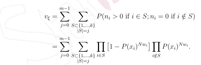
probability that all outcomes at either one (or both) of the design points are missing. For more complicated scenarios, this probability can be calculated as follows (see Imhof et al., 2002):

vξ = m−1

X

j=0

X

S⊂{1,...,k} |S|=j

P(ni >0 ifi∈S;ni = 0 if i /∈S)

=

m−1

X

j=0

X

S⊂{1,...,k} |S|=j

Y

i∈S

1−P(xi)N wi Y

i /∈S

P(xi)N wi.

We see that vξ is consistently smaller when adopting the second order

Table 2: Optimal designs found by using 1st and 2nd order Taylor series approximations to (4) respectively, for the optimality criterion denoted by the subscript, forn= 30 and

logistic MAR mechanism withγ0=−4.572 andγ1= 3.191. The other support point is x∗₁ = 0 withw1= 1−w2 andP(x∗1) = 0.01. ξ is theA-, c-, and D-optimal design that

assumes fully observed responses.

ξ∗

A2nd ξ

∗

A1st ξ∗c2nd ξ

∗

c1st ξD∗ 2nd ξ

∗

D1st ξ

x∗2 1.4630 1.51466 1.5497 1.60059 1.3360 1.37660 2 w2 0.4664 0.4539 0.6257 0.6208 0.5110 0.5 0.5 P(x∗2) 0.5241 0.5650 0.5922 0.6308 0.4234 0.4553 0.8594 vξ 1.186 e-04 3.378 e-04 5.359 e-05 0.0001577 1.897 e-06 7.4897 e-06 0.10302 space, here assumed to be [0,2]. Clearlyvξ is considerably higher here than

for other designs, and is motivation for considering the potential for missing data at the design stage of an experiment.

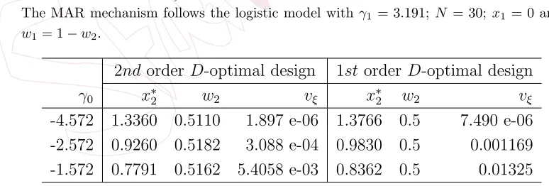
To investigate the issue of possible singularity of the covariance ma-trix further, we consider the effect of varying the parameter values for the missing data mechanism, resulting in different probabilities of missingness at the design points. Table 3 shows some examples of vξ computed using

the D-optimal designs for the simple linear model found for the different approximation methods with logistic MAR mechanisms. As the probability of a response being missing increases (i.e. γ0 becomes larger), the optimal designs found by the first order approach have a consistently higher failure rate in estimating the model parameters.

Table 3: Probabilities vξ for D-optimal designs found using different approximations.

The MAR mechanism follows the logistic model withγ1 = 3.191;N = 30; x1 = 0 and w1= 1−w2.

2ndorder D-optimal design 1storder D-optimal design

γ0 x∗2 w2 vξ x∗2 w2 vξ

-4.572 1.3360 0.5110 1.897 e-06 1.3766 0.5 7.490 e-06 -2.572 0.9260 0.5182 3.088 e-04 0.9830 0.5 0.001169 -1.572 0.7791 0.5162 5.4058 e-03 0.8362 0.5 0.01325

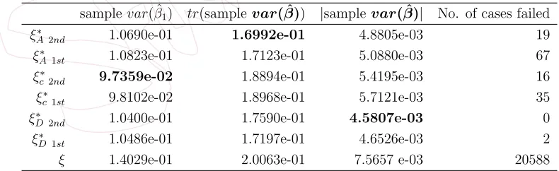
repeatedly simulate the incomplete data 200000 times as described above, setting σ2 _{= 1. In each incomplete data set, we empirically obtain the} covariance matrix for βˆ across the replications. Table 4 summarises the performance of the designs derived under the different optimality criteria and approximations. We see that the designs obtained under A-optimality have the smallest trace of the covariance matrix for βˆ, as expected. Fur-ther, this trace is smaller when using the design obtained from the second order approximation rather than the first order approximation. This pat-tern is repeated for the other optimality criteria. The design obtained un-der c-optimality from the 2nd order approximation results in the smallest variance for ˆβ1, and the design obtained under D-optimality from the 2nd order approximation results in the smallest determinant of the covariance matrix for βˆ. The design that assumes fully observed outcomes performs the worst across all optimality criteria, it also has the greatest proportion of cases where it was not possibly to estimate the regression coefficients, as expected, which highlights the importance of considering the potential for missing data at the design stage, to extract the most information out of an experiment. In addition, we also note that the second order approximation consistently resulted in fewer cases where it was not possible to estimate the parameters due to the missing data, and reflects what is seen in Table 2. This is further motivation for adopting the 2nd order approximation over the 1st order here.

Table 4: Simulation outputs of 200000 replications for different designs. The numbers in the last row indicate the frequency of the cases whereM(ξ,R) becomes singular.

samplevar( ˆβ1) tr(samplevar( ˆβ)) |samplevar( ˆβ)| No. of cases failed

ξA∗ 2nd 1.0690e-01 1.6992e-01 4.8805e-03 19

ξA∗ 1st 1.0823e-01 1.7123e-01 5.0880e-03 67

ξ∗

c2nd 9.7359e-02 1.8894e-01 5.4195e-03 16

ξ∗

c1st 9.8102e-02 1.8968e-01 5.7121e-03 35

ξ∗

D2nd 1.0400e-01 1.7590e-01 4.5807e-03 0

ξ∗

D1st 1.0486e-01 1.7197e-01 4.6526e-03 2

We have empirically evaluated our framework to construct optimal de-signs in the presence of missing values and found that our method worked well in the simulations, with evidence suggesting that it has the poten-tial to provide better approximations and hence result in better designs. Moreover, in all scenarios we investigated, the probability of a singular co-variance matrix was lowest for the optimal design using the second order approximation. In the next section we consider a scenario motivated from an application concerned with designing a clinical trial to treat Alzheimer’s disease.

5. Application: Redesigning a study on Alzheimer’s disease To illustrate an application of our approach, we use data from an Alzheimer’s disease study which investigated the benefits of administer-ing the treatments donepezil, memantine, and the combination of the two, to patients over a period of 52 weeks, on various quality of life measures. See Howard et al. (2012) for full details of the study. The total number of patients included in the primary intention-to-treat sample was 291, with 72 in the placebo group (Group 1), 74 in the memantine treatment group (Group 2), 73 in the donepezil treatment group (Group 3), and 72 in the donepezil-memantine group (Group 4).

In the per-protocol analysis, 43 patients were excluded in Group 1, 32 in Group 2, 23 in Group 3 and 21 in Group 4. Considering these patients as data missing at random, a logistic regression model is fitted to the data, specifically

P(Ri = 1|xi, vi) =

exp(γ0+γ1xi+γ2vi)

1 +exp(γ0+γ1xi+γ2vi)

wherexi, vi ∈ {0,1}represent the level of donepezil and memantine

respec-tively (with 1 indicating the treatment is applied) for patient i. From the data the regression coefficients were estimated to be ˆγ0 = 0.26365, ˆγ1 =

−0.89888 and ˆγ2 =−0.41085. We assume a linear regression model will be fit to the data, i.e.

Yi =β0+β1xi+β2vi+i, i ∼N(0, σ2), i= 1, . . . , n, (1)

is known and fixed to 1 without loss of generality. The specific values of

β0, β1, β2 will not affect the performance of the different designs. We can define the four groups (G1 - G4) the units are allocated to in terms of the design variablesx and v:

• G1: x∗i = 0, vi∗ = 0 with n1 experimental units;

• G2: x∗i = 0, vi∗ = 1 with n2 experimental units;

• G3: x∗i = 1, vi∗ = 0 with n3 experimental units;

• G4: x∗i = 1, vi∗ = 1 with n4 experimental units.

In this situation we have thus fixed the design points, defined by the values of (x, v) and equal to (0,0), (0,1), (1,0), and (1,1). The design problem is then to find the optimal number of patients to allocate to Groups G1

-G4, denoted by n1, n2, n3, and n4 respectively, under the assumption the analyst fits a linear regression model of the form described in (1) using the complete cases. The A-optimal design for this model minimises an appropriate approximation to

E{[M(ξ,R)−₍₁1_,1)]}+E{[M(ξ,R)−₍₂1_,2)]}+E{[M(ξ,R)−₍₃1_,3)]}

= E

Z1Z2+Z1Z3+ 2Z1Z4+ 3Z2Z3+ 2Z2Z4+ 2Z3Z4

Z1Z2Z3+Z1Z2Z4+Z1Z3Z4+Z2Z3Z4

whereZk = P

r∈Gk(1−Rr) is the sum of the response indicators for Group

Gk, k = 1, . . . ,4, subject to the constraints P4

k=1wk = 1 (equivalent to

n1+n2+n3+n4 =n) andwk ≥0, k = 1, . . . ,4. Hence for each designξ, the

existence set is given byCξ ={R∈ {0,1}n; at least 3 of Z1, Z2, Z3, Z4 are> 0}. See Appendix A.4 for the derivation of the objective function for A -optimality. The corresponding expression for D-optimality is not given here, but it can be easily obtained through the use of analytical software such as Maple 17 orMathematica.

subject to the weight constraint. Table 5 shows the allocation scheme of aA -and aD-optimal design, denoted byξ∗_Aandξ∗_D respectively. In the example considered here, due to the large sample size, we did not find any significant differences between the designs obtained through the first and second order approximations and so we have not distinguished between both designs here. In addition, the probability the regression coefficients cannot be estimated here is small for both approximation approaches (less than 10−20_{), so there} is no significant drawback using the 1st order approximation.

Table 5: A- andD-optimal designs for the Alzheimer’s example. The numbers in paren-theses indicate the expected number of missing values in the respective group.

n1 n2 n3 n4 n

w1 w2 w3 w4

ξ_A∗ 108(61.1) 64(29.6) 64(22.2) 55(14.3) 291 0.371 0.220 0.219 0.190

ξ_D∗ 60(33.9) 72(33.4) 78 (27.0) 81(21.1) 291 0.206 0.248 0.268 0.278

Using the same procedure as in Section 4, we assess the performance of the optimal designs by simulating incomplete data from the different designs using (1) above, choosing values of β0, β1, β2 to be 1,1,1 respec-tively. The missing values are introduced into the response using the MAR mechanism specified above. From each incomplete data set, regression co-efficients ˆβ0,βˆ1,βˆ2 are estimated from the complete cases. We repeat this process 350000 times, which allows us to empirically obtain the covariance matrix for ˆβ for each design. The original design, ξori = (n1, n2, n3, n4) = (72,74,73,72), with expected missing observations (40.7,34.3,25.3,18.7) is also considered here for comparison.

poten-tially have improved performance if they had been applied. For example, the A-optimal design would be expected to achieve a similar trace of the sample covariance matrix as the original design, while requiring only 95.55% of the overall sample size, or 13 fewer patients.

Table 6: Simulated values for the A- and the D-objective function, respectively, for

different designs.

A-optimality D-optimality

ξ_A∗ 0.066327 3.722e-06

ξ_D∗ 0.072111 3.3028e-06

ξori 0.069416 3.3439e-06

6. Discussion and remarks

We have proposed a theoretical framework for designing experiments that takes into account the possibility of missing values. Our framework broadens the approach proposed by Imhof, Song and Wong (2002), which is in fact a special case of our methodology that only takes a Taylor ex-pansion of order one, and does not take into account the potential issue of non-existence of the covariance matrix. We have provided a solid theoreti-cal grounding for our approach, and have illustrated the potential benefits through a simulation study.

For large sample sizes, the two approaches tend to lead to similar de-signs since non-existence is less of an issue, and the first and second order expansions are also similar. In these situations the first order approach might be preferred for practical reasons. The sample size of 30 we consid-ered in Section 4 is typical for Phase II clinical trials, where sample sizes are normally no more than 50. In this situation our investigation in Section 4 showed that the 2nd order approximation offered various benefits over the 1st order. We have also noted some further theoretical properties of using an approach based on the first order expansion and derived the necessary results in this article.

mod-els for simplicity. In these situations, the necessary Taylor expansions could easily be derived by hand. For more complicated linear models, in partic-ular if the size of the covariance matrix is large, it is recommended to use symbolic computation software, such as Mathematica, for deriving the sec-ond order approximation. Numerical computation of optimal designs will be challenging since convexity of the objective function is not guaranteed, but is feasible e.g. using metaheuristic search algorithms such as PSO; see, e.g., Chen et al. (2015).

Our methodology is also applicable to nonlinear and generalised lin-ear regression models. For nonlinlin-ear regression models with normally dis-tributed errors, this can readily be seen by considering linearisation of the regression function; see e.g. Atkinson, Donev and Tobias (2007), Chapter 17.2. More generally, the equality from (1) will only hold approximately. So while the framework is still applicable, this will add another level of approximation.

We have assumed that complete case analysis will be applied. While for many types of models such as regression models under a MAR mechanism, parameter estimates will be unbiased, there are other ways to handle the missing value problem, e.g. multiple imputation. Analysing the incomplete data in this way will not necessarily lead to the same designs derived in this article, which is an interesting area for future research. Another challenging scenario for future research arises when the assumption of MAR can no longer be expected to hold.

Supplementary Material

The derivations for Conjecture 4 can be found in the online supplement.

Acknowledgement

improve-ments of this paper. Appendix

A.1 Proof of Theorem 1. We can prove that the D-optimal design has

p+ 1 support points using the general equivalence theorem, by finding a contradiction. Assume ξ∗ has p+ 2 support points. Consider

g(x) := f

T

(x)M−1(ξ∗) f(x)

p+ 1 ≤

1

1−P(x) :=h(x)

whereg(x) is a polynomial of degree 2p, which has to be less than h(x) over the region [l, u]. We order the p+ 2 values forx by size:

l≤x∗₁ < x∗₂ < ... < x∗_p+2 ≤u (1)

such that the above equality is achieved. This implies g(x∗_i) touches h(x∗_i) and g0(x∗_i) = h0(x∗_i) for i = 2,3, ..., x∗_p+1. From (1), there are values

x₁∗0, ..., x∗_p0₊₁ with g0(x∗_i0) = h0(x_i∗0) such that x∗₁ < x∗₁0 < x∗₂ < x∗₂0 < x∗₃ < ... < x∗_p+1 < x∗_p0₊₁< x∗_p+2 by the Mean Value Theorem.

Hence we have a total of 2p+ 1 values whereg andh have equal deriva-tives, andg0(x) is a polynomial of degree 2p−1. Applying the Mean Value Theorem again to g0 and h0, there must be 2p values where g00 and h00 are equal. By repeating this process, we find that there must be 2 values where the 2pth _derivativesg(2p) _andh(2p) _{are equal, andg}(2p)_{(x) is a constant since}

g is a polynomial of degree 2p. This is a contradiction since we assumed that h(2p)(x) = c has at most one solution in < for any constant c. The same contradiction occurs if we assume ξ∗ has more than p + 2 support

points.

A.2 Second order Taylor series approximation. Let X be a discrete random variable with expectation X. We expand H(X) = 1/X about the point X into a second order Taylor series:

H(X)≈ 1

X −

X−X

X2

+(X−X) 2

X3 .

Since E{(X−X)}= 0 and E{(X−X)2_{}=V ar(X),E{H(X)} ≈} 1

E[X]+

V ar(X)

E[X]3 . For the zero truncated binomial random variableZj with moments

E[Zj] =

nwj(1−P(x∗j))

1−P(x∗

j)nwj

V ar(Zj) =

nwj(1−P(x∗j))[P(x∗j)− {P(xj∗) +nwj(1−P(x∗j))}P(x∗j)nwj]

(1−P(x∗_j)nwj₎2 ,

we obtain E 1 Zj ≈ 1

E{Zj}

+ V ar(Zj) (E{Zj})3

= (1−P(x

∗

j)nwj)2{P(x

∗

j) +nwj(1−P(x∗j))}

(nwj)2(1−P(x∗j))2

.

A.3 Proof of part (a) of Theorem 3. Let without loss of generality

x∗₁ < x∗₂, denote nwj by nj, j = 1,2 where nj is a positive integer, and

assume P(x) is monotone increasing in x.

Step 1: We show that the second order approximation toE[1/Z1] is increas-ing in x∗₁ forn1 ≥2 and constant forn1 = 1.

Denote the right hand side of (5) for E[1/Z1] (times n21) byfn1(P), and

note that for increasingP(x), it suffices to show that for all n1 ≥2,fn1(P)

is increasing in P ∈(0,1). Moreover, (1−Pn1_)/(1−_{P) =} Pn1−1

k=0 P

k_{, so}

fn1(P) = (

n1−1

X

k=0

Pk)2[P +n1(1−P)]

with derivative

f_n0

1(P) = (

n1−1

X

k=0

Pk)

2

n1−2

X

k=0

(k+ 1)Pk

{P +n1(1−P)}+ (1−n1)

n1−1

X

k=0

Pk

.

The first factor is positive. Rearranging the term in square brackets yields

2n1

n1−2

X

k=0

(k+ 1)Pk

+ 2(1−n1)

n1−1

X

k=1

kPk

+ (1−n1)

n1−1

X

k=0

Pk

= n1+ 1 +

n1−2

X

k=1

Pk{n1+ 1 + 2k}

+Pn1−1_{(1−n)(2n−1)}

≥ Pn1−1

n1+ 1 +

n1−2

X

k=1

{n1+ 1 + 2k}

+ (1−n)(2n−1)

= 0

sincePn1−1 ≤_{1 andP}n1−1 ≤_Pk_fork≤_n

x∗₁ = l. If n1 = 1, fn1(P) = 1, since the zero truncated Binomial random

variable Z1 can only take the value 1.

Step 2: The second order approximation forE[1/Z2] does not depend onx∗₁. Since x∗₁ = l minimises 1/(x∗₁ −x∗₂)2, and all expressions are non-negative, the objective functions in (7) and (8) are both minimised when x∗₁ =l. If

l ≥ 0, (x∗2

1 + 1) is also increasing in x∗1, and the result for A-optimality follows.

An analogous argument shows that x∗₂ =u minimises (7), (8) and, for

u≤0, also (9) if P(x) is monotone decreasing. Proof of Theorem 3(b). The right hand side of (6) does not depend on the support points. Hence the objective functions in (7) and (8), respec-tively, are minimised with respect tox∗₁ andx∗₂ when the factor 1/(x∗₁−x∗₂)2 is minimised. This is achieved by setting x∗₁ =l and x∗₂ =u.

Taking partial derivatives in (9) with respect tox∗₁ and x∗₂, respectively, shows that regardless of the values of the expression in (6) the derivative with respect to x∗₁ (x∗₂) is non-negative (non-positive) if l ≥ 0 or u ≤ 0. Hence theA-objective function is minimised whenx∗₁ =l and x∗₂ =u. A.4 The covariance matrix from the Alzheimer’s example

[M(ξ,R)]−1 = 1

|M(ξ,R)|

Z2Z3+Z2Z4+Z4Z3 −(Z2+Z4)Z3 −(Z3+Z4)Z2

−(Z2+Z4)Z3 (Z2+Z4)(Z1+Z3) −Z4Z1−Z2Z3

−(Z3+Z4)Z2 −Z4Z1−Z2Z3 (Z3+Z4)(Z1+Z2)

!

where |M(ξ,R)|=Z1Z2Z3+Z1Z2Z4+Z1Z3Z4+Z2Z3Z4, with trace

Z1Z2+Z1Z3+ 2Z1Z4+ 3Z2Z3+ 2Z2Z4+ 2Z3Z4

Z1Z2Z3+Z1Z2Z4+Z1Z3Z4+Z2Z3Z4

where Zk =P_i∈Gk(1−Ri) is the sum of the response indicators in Group

Gk, k = 1, . . . ,4. A bivariate second order Taylor expansion of F/G about

E[F] andE[G], whereF =Z1Z2+Z1Z3+ 2Z1Z4+ 3Z2Z3+ 2Z2Z4+ 2Z3Z4 and G=Z1Z2Z3+Z1Z2Z4+Z1Z3Z4+Z2Z3Z4, yields

E

F G

≈ E{G

2_}E{F} (E{G})3 −

E{F G}

(E{G})2 +

E{F}

E{G}.

distributions for allZ1, Z2, Z3 andZ4, when for existence only three of them would have needed to be truncated. This is justified due to the large sample size.

References

Ahmad, T., and Gilmour, S. G. (2010). Robustness of subset response sur-face designs to missing observations. Journal of Statistical Planning and Inference,140(1), 92-103.

Baek, I., Zhu, W., Wu, X., and Wong, W. K. (2006). Bayesian optimal designs for a quantal dose-response study with potentially missing observations. Journal of Biopharmaceutical Statistics, 16(5), 679-693.

Bang, H., and Robins, M. J. (2005). Doubly robust estimation in missing data and causal inference models. Biometrics, 61(4), 962-973.

Carpenter, J. R., Kenward, M. G., and White, I. R. (2007). Sensitiv-ity analysis after multiple imputation under missing at random: a weighting approach. Statistical Methods in Medical Research, 16(3), 259-275.

Chen, R. B., Chang, S. P., Wang, W., Tung, H. C. and Wong, W. K. (2015). Minimax optimal designs via particle swarm optimization methods. Statistics and Computing,25(5), 975-988.

De la Garza, A. (1954). Spacing of information in polynomial regression.

The Annals of Mathematical Statistics, 25(1), 123-130.

Fedorov, V. V. (1972). Theory of optimal experiments. Elsevier

Ghosh, S. (1979). On robustness of designs against incomplete data. Sankhy¯a: The Indian Journal of Statistics, Series B, 204-208.

Hackl, P. (1995). Optimal design for experiments with potentially failing trials. In Proc. of MODA4: Advances in Model-Oriented Data Anal-ysis (Edited by C. P. Kitsos and W. G. M¨uller), 117-124. Physica Verlag, Heidelberg.

Hedayat, A. and John, P. W. M. (1974). Resistant and susceptible BIB designs. The Annals of Statistics , 2(1), 148–158.

Herzberg, A. M. and Andrews, D. F. (1976). Some considerations in the optimal design of experiments in non-optimal situations. Journal of the Royal Statistical Society: Series B (Methodological), 38, 284-289.

Howard, R., McShane, R., Lindesay, J., Ritchie, C., Baldwin, A., Bar-ber, R., ... and Phillips, P. (2012). Donepezil and memantine for moderate-to-severe Alzheimer’s disease. New England Journal of Medicine, 366(10), 893-903.

Ibrahim, J. G. and Lipsitz, S. R. (1999). Missing covariates in general-ized linear models when the missing data mechanism is non-ignorable.

Journal of the Royal Statistical Society: Series B (Methodological), 61(1), 173-190.

Imhof, L. A and Song, D. and Wong, W. K. (2002). Optimal design of experiments with possibly failing trials. Statistica Sinica, 1145-1155.

Imhof, L. A and Song, D. and Wong, W. K. (2004). Optimal design of experiments with anticipated pattern of missing observations. Journal of Theoretical Biology,228(2), 251-260.

Kenward, M. G., Molenberghs, G., and Thijs, H. (2003). Pattern mixture models with proper time dependence. Biometrika,90(1), 53-71.

Little, R. J. A. (1992). Regression with missing X’s: a review. Journal of the American Statistical Association, 87(420), 1227-1237.

Little, R. J. A. and Rubin, D. B. (2002). Statistical analysis with missing data. J. Wiley.

Mitra, R. and Reiter, J.P. (2011). Estimating propensity scores with miss-ing covariate data usmiss-ing general location mixture models. Statistics in Medicine, 30(6), 627-641.

Mitra, R. and Reiter, J.P. (2016). A comparison of two methods of estimat-ing propensity scores after multiple imputation. Statistical Methods in Medical Research, 25(1), 188-204.

Ortega-Azurduy, S. A., Tan, F. E. S. and Berger, M. P. F. (2008). The effect of dropout on the efficiency of D-optimal designs of linear mixed models. Statistics in Medicine,27(14), 2601-2617.

Pukelsheim, F. (2006). Optimal design of experiments (Classics in Ap-plied Mathematics). Society for Industrial and Applied Mathematics, Philadelphia, PA, USA

Pukelsheim, F. and Rieder, S. (1992). Efficient rounding of approximate designs. Biometrika, 79(4), 763-770.

Rubin, D.B (1976). Inference and missing data. Biometrika, 63(3), 581-592.

Rubin, D. B. (1987). Multiple imputation for nonresponse in surveys.

Wiley-Interscience.

Schafer, J. L. (1997). Analysis of incomplete multivariate data. CRC press.

Silvey, S. D. (1980). Optimal design. Chapman and Hall, London.