Robust volatility estimation for multiscale diffusions with zero quadratic variation

warwick.ac.uk/lib-publications

A Thesis Submitted for the Degree of PhD at the University of Warwick

Permanent WRAP URL:

http://wrap.warwick.ac.uk/111074

Copyright and reuse:

This thesis is made available online and is protected by original copyright.

Please scroll down to view the document itself.

Please refer to the repository record for this item for information to help you to cite it.

Our policy information is available from the repository home page.

Robust Volatility Estimation for Multiscale

Diusions with Zero Quadratic Variation

by

Theodoros Manikas

Thesis

Submitted to the University of Warwick

for the degree of

Doctor of Philosophy

Department of Statistics

Contents

List of Tables iv

List of Figures vi

Acknowledgments viii

Declarations ix

Abstract x

Chapter 1 Introduction 1

1.1 Parameter Estimation for Multiscale Diusions . . . 3

1.1.1 MLE and Quadratic Variation . . . 3

1.2 Volatility Estimation for HighFrequency Financial Data . . . 6

1.3 Aim and Objectives . . . 9

1.4 Outline of the Thesis . . . 9

Chapter 2 Obtaining CoarseGrained Models from Multiscale Diu-sions 11 2.1 Introduction . . . 11

2.2 Averaging and Homogenization for SDEs . . . 12

2.2.1 Limiting equations for multiscale diusions . . . 13

2.2.1.1 Averaging . . . 13

2.2.1.2 Homogenization . . . 14

2.3 Summary . . . 15

Chapter 3 The Extrema Quadratic Variation 16 3.1 Types of Quadratic Variation . . . 16

3.1.1 Quadratic Variation . . . 16

3.1.3 Extrema Quadratic Variation (ExtQV) . . . 17

3.2 Computation of (ExtQV) in practice . . . 18

Chapter 4 Diusion Coecient Estimation for a Simple Multiscale Ornstein-Uhlenbeck Process 21 4.1 The Model . . . 21

4.2 Analytical Proof of Theorem 4.1 . . . 23

4.2.1 The rst term . . . 25

4.2.2 The second the third term . . . 31

4.2.3 The fourth term . . . 32

4.3 Numerical Results . . . 32

4.3.1 Unbiasedness of the Exrema Quadratic Variation . . . 33

4.3.2 Consistency of the Extrema Quadratic Variation . . . 34

4.4 Summary . . . 36

Chapter 5 General Bounded Variation Model 38 5.1 The General Model . . . 38

5.2 Analytical Proof of Theorem 5.3 . . . 40

5.3 Homogenization with Drift . . . 50

5.4 Summary . . . 51

Chapter 6 Simulation Study 52 6.1 Examples . . . 52

6.2 Summary . . . 67

Chapter 7 Extrema Quadratic Variation for Multiscale Diusions with Bounded Quadratic Variation 69 7.1 Extrema Quadratic Variation for the Brownian Motion . . . 69

7.2 Extrema Quadratic Variation for Multiscale Diusions with Bounded Quadratic Variation . . . 73

7.3 Summary . . . 74

Chapter 8 Conclusions and Future Work 76 8.1 Thesis Summary . . . 76

8.2 Future Work . . . 78

Appendix A Useful Tools 85

B.1 More Numerical Results for Chapter 4 . . . 92

List of Tables

4.1 Expectation of the (ExtQV) for the model (4.1). Investigation of its behavior for dierent n's and's and for σ = 1. . . 33 4.2 L2error of the (ExtQV) for data generated by the model (4.1).

In-vestigation of its behavior for dierent n's and's and for σ= 1. . . 36

6.1 Expectation andL2error of the (ExtQV) for data generated by (6.1). Investigation of its behavior for dierent n's and's and for σ = 0.10. 59 6.2 Expectation and L2error of the (ExtQV) for data generated by the

model in the Example 6.2. Investigation of its behavior for dierent n's and's and for σ= 1. . . 63 6.3 Expectation and L2error of the (ExtQV) for dierent 's, n's and

σ =√0.5. . . 65 6.4 Expectation and L2error of the (ExtQV) for data generated by the

model in the Example 6.4. Investigation of its behavior for dierent n's and's and for σ= 1. . . 67

7.1 Expectation of the (ExtQV) for the Brownian motion process for dif-ferent n's. Comparison between its numerical and theoretical value. . 73 7.2 Expectation of the (ExtQV) for data generated by the model (7.8).

Investigation of its behavior for dierent n's and's. . . 74 7.3 Expectation of (ExtQV) when applied to data from the model (7.8).

Investigation of its behavior for dierent n's, σ1's, σ2's and for = 21/4

√

n. . . 74

List of Figures

3.1 Visualization of an extremal point . . . 18 3.2 Visualization of the notion of the extremal path . . . 18

4.1 Expectation of the (ExtQV) for the model (4.1). Investigation of its behavior for dierent n's and's and for σ = 1. . . 34 4.2 Expectation of the (ExtQV) for the model (4.1). Investigation of its

behavior for dierent 's and for xedn= 106 and σ= 1. . . 35 4.3 Expectation of the (ExtQV) for the model (4.1). Investigation of its

behavior for dierent 's and for xedn= 106 and σ= 2. . . 35 4.4 Expectation of the (ExtQV) for the model (4.1). Investigation of its

behavior for dierent σ's and for xedn= 106 and= 0.10. . . 36 4.5 Investigation of the L2error behavior with respect to through a

loglog plot . . . 37

6.1 Expectation of the (ExtQV) for the model (6.1). Investigation of its behavior for dierent 's and for xedn= 106 and σ= 0.1. . . 60 6.2 Expectation of the (ExtQV) for the model (6.1). Investigation of its

behavior for dierent 's and for xedn= 106 and σ= 0.5. . . 61 6.3 Expectation of the (ExtQV) for the model in the Example 6.2.

Inves-tigation of its behavior for dierent n's and's and for xed n= 106 and σ = 1. . . 64 6.4 Expectation of the (ExtQV) for the model in the Example 6.3.

Inves-tigation of its behavior for dierent n's and's andσ = 0.5. . . 65 6.5 Expectation of the (ExtQV) for the model in the Example 6.3.

In-vestigation of its behavior for dierent 's, constant n= 106 and for σ = 0.5. . . 66 6.6 Expectation of the (ExtQV) for the model in the Example 6.4.

Acknowledgments

First and foremost I would like to thank my supervisor, Dr. Anastasia Papavasiliou, for all her assistance and guidance. I will always be grateful to her for the opportunity she gave me to work in an ideal and stimulating environment. I am also grateful to the Warwick Statistics department for funding my PhD studies.

Special thanks goes to my friends and atmates Pantelis and Panayiota who made my life easier and my free time much more enjoyable. They will be one of the reasons to remember Warwick as a pleasant experience in my life.

Also, I would like to express my deepest gratitude to my family members, my parents, Yiannis and Dimitra, my sister Antigoni, and my aunt, Lola. I never would have made it here without their unconditional love, support and encouragement.

Declarations

This thesis is submitted to the University of Warwick in support of my application for the degree of Doctor of Philosophy. It has been composed by myself except when stated otherwise and has not been submitted in any previous application for any degree.

Abstract

CHAPTER

1

Introduction

In many application areas, it is often the case that the most accurate models to describe the dynamics of a physical phenomenon are multiscale in nature. Such situations can be met in the eld of molecular dynamics (Schlick, 2010), in atmo-sphere/ocean science; see, for example, Majda et al. (2001, 2006) and Katsoulakis et al. (2004, 2005) and in network trac data (Abry et al., 2002). Also, especially in the elds of econometrics, highfrequently observed nancial data exhibit multiscale characteristics in the sense that dierent features are associated with dierent time scales. These features are usually described by the term market microstructure noise, which contains all dierent types of market inconsistencies such as non-synchronous trading and bidask spread. Tsay (2005) described each of these eects and give a comprehensive review.

Finding a coarsegrained model that can eectively describe the dynamics of the initial multiscale model is a very popular problem among applied mathematicians. This is mainly due to the fact that such models are much more ecient to use in practice. Once the coarsegrained model has been extracted, the corresponding free parameters are needed to be estimated by tting the model to the data. In this framework, the problem that one is confronted with is the mismatch between the coarsegrained model and the data generated by the full multiscale system.

types similarly to Pavliotis and Stuart (2008). For the averaging one has

dx=f1(x, y)dt+a0(x, y)dU+a1(x, y)dV, x(0) =x0, (1.1a)

dy= 1

g0(x, y)dt+ 1 √

β(x, y)dV, y(0) =y0, (1.1b)

and for the homogenization,

dx=

1

f0(x, y) +f1(x, y)

dt+a0(x, y)dU+a1(x, y)dV, x(0) =x0, (1.2a)

dy=

1

2g0(x, y) + 1

g1(x, y)

dt+ 1

β(x, y)dV. y(0) =y0, (1.2b)

where0 < << 1 denotes a small parameter controlling the scale separation, and U, V are independent standard Brownian motions. In both cases, the process x should be viewed as a process evolving on a timescale which is much slower that the timescale of y. For this reason, the process x will be usually referred as the slow variable of the system whereasyas the fast one. As mentioned earlier, the objective is to obtain a coarsegrained model describing the dynamics of the slow variable x. In Pavliotis and Stuart (2008), the reader can nd a comprehensive study of how using averaging or homogenization techniques it is possible to show that the slow process converges weakly (in the limit of → 0) to a process X solving an appropriate SDE

dX =F(X)dt+ Σ(X)dW, X(0) =x0. (1.3)

1.1 Parameter Estimation for Multiscale Diusions

The parameter estimation problem in the context of multiscale diusions has been examined extensively by several authors, see for example Pavliotis and Stuart (2007); Sykulski et al. (2008); Papavasiliou et al. (2009); Papavasiliou (2011); Krumscheid et al. (2013); Krumscheid (2014a); Papanicolaou and Spiliopoulos (2014); Kalliadasis et al. (2015); Krumscheid et al. (2015); Gailus and Spiliopoulos (2017a,b); Papani-colaou and Spiliopoulos (2017). A review of these papers will follow in the following sections.

The statistical estimation problem of our interest is to use datadriven techniques to t data from Eq.(1.1) or Eq.(1.2) to an SDE of the form

dX =F(X;θ)dt+ Σ(X)dW, X(0) =x(0), (1.4)

whereθis an unknown parameter. The standard approach for the estimation of the drift and diusion coecient in an SDE of the form (1.4) is the maximum likelihood estimator for the drift and the quadratic variation for the diusion coecient (see Bishwal (2008); Kutoyants (2013); Liptser and Shiryaev (2013)). However, it turns out that due to the small eects in the observations these estimators are not helpful. in the context of multiscale diusions. In fact, due to the small eects in the obser-vations these estimator are biased (see Theorem 1.1 in Pavliotis and Stuart (2007)). Also, Krumscheid (2014b) uses a simple example to illustrate the failure of these methods.

In the following subsection we are going to give an overview of these estimators.

1.1.1 MLE and Quadratic Variation

Following the work in Papavasiliou et al. (2009), we assume that Σ in Eq.(1.4) is uniformly positivedenite onX, Eq.(1.4) is ergodic with invariant measureν(dx) = π(x)dxat θ=θ0 and that

A∞:=

ˆ

X

is invertible. Then, given data{z(t)}_t∈[0,T] an application of the Girsanov theorem suggests that the log likelihood forθsatisfying Eq.(1.4) is given by

L(θ;z) =

ˆ T

0

hF(z;θ), dzi_α(z)−1 2

ˆ T

0

|F(z;θ)|2_α(z)dt, (1.6)

where

hp, qi_α(z)=

Σ(z)−1p,Σ(z)−1q

. (1.7)

Then, the maximum likelihood estimator (MLE) ofθgiven z is

ˆ

θ(z) =argmax_θL(θ;z). (1.8)

The quadratic variation on the other hand, for data given on nely spaced partition, π_(n)([0, T]), is

ˆ

Σ(z) = lim meshπ(n)([0,T])→0

n−1 X

i=0

(z(ti+1)−z(ti))2. (1.9)

Although in theory, subsampling the available data may lead to consistent estima-tions for the parameters of the limiting equaestima-tions, the question of how to nd an optimal subsampling rate remains. Studies concerning the determination of this rate for Gaussian processes can be found in Azencott et al. (2010, 2011). In cases where the model describing the initial multiscale data is unknown, it is infeasible to nd this optimal rate and it is also consists the MLE approach inappropriate.

In the context of the diusion estimation problem for a simple OrnsteinUhlenbeck multiscale system, Papavasiliou (2011) tried to overcome this problem by introduc-ing the pvariation estimate, a notion relying in the theory of rough paths Lyons (1998); Lyons and Qian (2002). It was shown that the proposed estimator which provided a nonparametric way of subsampling the data was asymptotically unbi-ased and furthermore itsL2error performance was better than the one proposed in Pavliotis and Stuart (2007); Papavasiliou et al. (2009). Apart from the fact that this methodology was developed in the context of a particular example it also lacks of practical usability. The result was proven in a pure theoretical and continuous time framework and it is not easily interpretable in a reallife framework. For example, given data how could one compute their pvariation, i.e., the supremum over all possible partitions? The aim of the work presented here is to address this issue and to extend this methodology to a more general framework.

Other methodologies in the direction of addressing the issue of the optimal subsam-pling rate have been presented in Krumscheid et al. (2013); Krumscheid (2014a); Kalliadasis et al. (2015). Based on the computational studies in Krumscheid et al. (2013); Krumscheid (2014a) and Kalliadasis et al. (2015) developed a methodology on obtaining a functional relation between the unknown parameterθand the statis-tical properties of the model in Eq.(1.4). Then, an estimator of θ was derived via the best approximation of a system of equations. The resulting estimator was shown to be robust with respect to weak pertubations.

1.2 Volatility Estimation for HighFrequency Financial

Data

Highfrequency nancial data are dened as intraday data observed on the prices of nancial assets. Nowadays, the advances in technology allow the wide use of high frequency nancial data from dierent nancial markets and from individuals to buy and sell. This lead to an increasing demand for better modelling and statistical inference regarding the price and volatility dynamics of the assets.

In nancial applications, the most common modelling approach is the diusion pro-cess and the model is described as follows:

LetX(t) be the price process of a security (e.g. a stock price), then it is assumed that the log processY(t) := logX(t) follows an Itô process,

dY(t) =µ(t, Y(t))dt+σ(t, Y(t))dW(t), Y(0) =Y0, (1.10)

whereW is a standard Brownian motion and the functions µ(t, Y(t)) : [0, T] → _R and σ(t, Y(t)) : [0, T] → R are called the drift and the diusion coecient (or

volatility) respectively. Under local Lipshitz and linear growth conditions on the functionsµ and σ, a unique strong solution for the Eq.(1.10) can be derived. This solution is called diusion process and it is well known that it is a semimartingale. Semimartingales is a natural class of processes for modelling securities in a context that does not allow arbitrage opportunities, see Karatzas and Shreve (2012). The statistical estimation problem of our interest is the estimation of the diusion co-ecient (volatility). Various methodologies have been developed in the past several years to estimate the integrated volatility. For an overview see the survey by Ander-sen et al. (2002). The classical nonparametric approach to estimate the integrated volatility is via the quadratic variation of the observations from model (1.10). The latter is usually referred as realised variance or realised volatility. In fact, classi-cal stochastic processes theory suggests that as the sampling frequency increases, the estimation error of the realised variance should be diminished (Karatzas and Shreve, 2012). Based on this, naturally one would believe that in a highfrequency context the realised variance would perform with a negligible estimation error.

to go to innity (Brown, 1990; Hansen and Lunde, 2006) and more general, for the appropriateness of the realised variance see Barndor-Nielsen and Shephard (2002); Andersen et al. (2003) In particular, the bias problem is apparent from volatility sig-nature plots, namely plots of realised volatility versus alternative sampling frequen-cies, that were introduced by Andersen et al. (2000). The reason for this anomaly is the fact that the realised variance yields a perfect estimate for the volatility in the hypothetical scenario where prices are observed in continuous time and without measurement errors (Jacod and Shiryaev, 2013). In practice, this is not the case and Awartani et al. (2004) described the fact that there is noise contaminating the data. Also, a very recent study on testing whether a highfrequency data sample can be treated as reasonably free of market microstructure noise at a given sampling frequency has been presented in Ait-Sahalia and Xiu (2017). Based on the above heuristics we may conclude that Eq.(1.10) is not the appropriate modeling approach for highfrequency data and one should seek for alternative models.

The volatility estimation problem for nancial data that are contaminated by the market microstructure noise has been studied extensively in literature. Indicatively see Zhou (1996); Corsi et al. (2001); Aït-Sahalia et al. (2005); Zhang et al. (2005); Barndor-Nielsen et al. (2008); Bandi and Russell (2008); Jacod et al. (2009) and references therein. The common modelling approach in these studies is the following model

Y(t) =X(t) +(t), (1.11)

whereX follows Eq.(1.10) andstands for the noise around Y.

There are ve main approaches in literature for the estimation of the integrated volatility under the presence of microstructure noise:

• autocovariance based introduced by Zhou (1996)

• subsampling introduced by Zhang et al. (2005)

• realized kernel methods introduced by Barndor-Nielsen et al. (2008a,b)

• likelihood approach introduced by Aït-Sahalia et al. (2005)

• preaveraging techniques introduced by Podolskij et al. (2009); Podolskij and Vetter (2009).

However, the main disadvantage of this approach is the inconsistency.

A non-parametric approach based on subsampling was proposed by Zhang et al. (2005). These authors proposed the twoscale realised volatility estimator which was the rst consistent estimator of the integrated volatility under the presence of microstructure noise. An extension of this estimator can be found in Zhang et al. (2006) with the multiscale volatility estimator and later on Aït-Sahalia et al. (2011) improved the eciency of the estimator. In fact, it was shown that the multiscale estimator converges to the true value of the integrated volatility at the rate ofn1/4 whereas the twoscale converges at a rate ofn1/6.

The realized kernel methods developed in Barndor-Nielsen et al. (2008a) and their proposed estimator was also consistent and achieved a convergent rate of ordern1/4 as well. Same authors, Barndor-Nielsen et al. (2008b), extended their work for non-negative form of realised kernels where now the convergent rate was of ordern1/5but had the advantage of a non-negative kernel with probability one, which is generally not the case for the other estimators available in the literature. They derived the limit distribution under various assumptions on kernel weights and Barndor-Nielsen et al. (2009) applied the methodology of realised kernels in practice where they identied some challenges based on the features of high frequency data and focused on the crucial problem of the bandwidth selection for kernel methods. Recently, Barndor-Nielsen et al. (2011) combined the two very popular non-parametric approaches of subsampling and realised kernels and concluded that the combination of the two is highly advantageous for estimators based on discontinuous kernels, had no eect on kinked kernels and a negative eect for smooth kernels as it had as a result the increase of asymptotic variance.

The likelihood approach has been initiated by Aït-Sahalia et al. (2005) assuming constant volatility in order to be able to perform maximum likelihood estimator. Xiu (2010) extended this approach to allow stochastic volatility. The latter author demonstrated that the parametric likelihood approach is consistent, ecient and robust with respect to stochastic volatility. Also it has the same model-free feature as the non-parametric approaches i.e. subsampling and realised kernels with the main advantage of the nite sample performance.

Jumps are an extension of the model and according to discussions in Jacod and Protter (2012) and Aït-Sahalia and Jacod (2014) both noise and jumps can have an impact on the statistical signicance. Recently Mykland and Zhang (2016) extended the preaveraging method and combined it with Mestimators. This methodology is robust against the noise and the jumps while averaging the continuous part.

1.3 Aim and Objectives

The aim of this thesis is to develop methodology for estimating the diusion coe-cient of a homogenized SDE when the data are modelled via multiscale diusions. We will assume data from a multiscale system of the form given in Eq.(1.2). Under the appropriate assumptions, model (1.2) converges in law to a limiting diusion process whose drift and diusion coecients can be found in Pavliotis and Stuart (2008, Chapter 11) or in Bensoussan et al. (2011). The work in this thesis diers from previous research in the area because it does not require the explicit value of the scale separation parameter to construct the proposed estimator.

Our aim is to demonstrate theoretical and numerical results to show the eciency of our proposed estimator for the diusion (volatility) coecient of the corresponding limiting diusion process.

1.4 Outline of the Thesis

The remainder of the thesis is organised as follows.

CHAPTER

2

Obtaining CoarseGrained Models from Multiscale

Diusions

In this chapter, the main concepts and methods used in this thesis are introduced. In particular, we review the methodology of extracting a coarsegrained models from multiscale diusions. We describe two classes of multiscale diusion processes, the averaging and homogenization for SDEs. However, the main focus of this thesis is the homogenization case as it the most popular in the literature for the parameter estimation problem. The content of this chapter relies on Pavliotis and Stuart (2008).

2.1 Introduction

2.2 Averaging and Homogenization for SDEs

To generate data with a multiscale character, the following two classes of multiscale diusion processes have been employed in the papers reviewed in Chapter 1. The rst is averaging for SDEs, where the data are generated for a system of SDEs with the following form

dx(t) =f1(x(t), y(t))dt+α0(x(t), y(t))dU(t) +α1(x(t), y(t))dV(t), x(0) =x0,

(2.1a)

dy(t) = 1

g0(x(t), y(t))dt+ 1 √

β(x(t), y(t))dV(t), y(0) =y0. (2.1b)

Later we are going to demonstrate that averaging f1 and α0αT0 over the invariant measure of theyprocess withxviewed as xed, the drift and the diusion coecient of the corresponding limiting diusion process are obtained. The second class is homogenization for SDEs and has the following form

dx(t) =

1

f0(x(t), y(t)) +f1(x(t), y(t))

dt

+α0(x(t), y(t))dU(t) +α1(x(t), y(t))dV(t), x(0) =x0, (2.2a)

dy(t) = 1

2g0(x(t), y(t))dt+ 1

g1(x(t), y(t))dt+ 1

β(x(t), y(t))dV(t), y(0) =y0, (2.2b)

where << 1, x ∈ X =Tl, y ∈ Y =Td−l (the l and d−l dimensional unit torus

respectively),U,V are independent standard Brownian motions of dimensionmand nrespectively,fi :X × Y →Rl(i∈ {0,1}),α0 :X × Y →Rl×n,α1 :X × Y →Rl×m,

gi(x, y) :X × Y →Rd−l (i∈ {0,1}) and β(x, y) :X × Y →R(d−l)×m.

As→0 and under the appropriate assumptions on the functionsf0,f1,g0 ,g1,α0,

α1 and β, the solution x(t) of both systems (2.1) and (2.2) converges in Lp (p >1) in the averaging, and in law in the homogenization case to the solution of a diusion process of the following form

dX(t) =F(X(t))dt+ Σ(X(t))dW(t), X(0) =x0, (2.3)

and diusion coecients respectively and their form can be extracted explicitly.

2.2.1 Limiting equations for multiscale diusions

In what follows the reader is referred to Pavliotis and Stuart (2008, Chapters 6, 17 and 18) for more details.

Letφt_ξ(y) be the Markov process solving the SDE

d(φt_ξ(y)) =g0(ξ, φtξ(y))dt+β(ξ, φtξ(y))dV(t), φ0ξ(y) =y0, (2.4)

whereg0 and β as dened above. Then, the generator of this process is

L₀(ξ) =g0(ξ, y)· ∇y+ 1

2β(ξ;y)β(ξ;y) T _:∇

y∇y. (2.5)

Notice that since Y = Td−l the operator L0 and its adjoint L∗0 are equipped with periodic boundary conditions. The adjoint of the operatorL₀ is given by

L∗₀=−∇_yg(ξ, y) +1

2∇y∇yβ(ξ;y)β(ξ;y) T_.

In the following subsections, we quote the necessary assumptions under which the averaging and homogenization problem converge to a limiting diusion process and we present the corresponding form of the drift and diusion coecients.

2.2.1.1 Averaging

Assumption 2.1. 1. The problem

−L∗₀(ξ)ρ∞(y;ξ) = 0 & ˆ

Y

ρ∞(y;ξ)dy= 1, (2.6)

has a unique non-negative solutionρ∞(y;ξ)∈L1(Y) for every ξ∈ X and also ρ∞(y;ξ) is C∞ both in y and ξ. This assumption assures us that the fast processes in the systems (2.1b) and (2.2b) are ergodic for eachξ∈ X.

2. The functions f0, f1, g0, g1, α0, α1, and β and all derivatives are uniformly bounded inX × Y.

by

Denition 2.2.

−L₀Φ(y;ξ) =f0(y;ξ),

ˆ

Y

Φ(y, ξ)ρ∞(y;ξ)dy= 0. (2.7)

Remark 2.3. Provided Y = Td−l and B(ξ, y) := β(ξ;y)β(ξ;y)T is positive denite

all the above assumption hold (see Pavliotis and Stuart (2008, Chapter 6)).

Given Assumption 2.1, deneF :X →_Rl as

F(X) = ˆ

Y

f0(x, y)ρ∞(y;x)dy, (2.8)

andΣ :X →_Rl×l as

Σ(X)Σ(X)T = ˆ

Y

α(x, y)α(x, y)Tρ∞(y;x)dy, (2.9)

in order for the following theorem to hold.

Theorem 2.4 (Pavliotis and Stuart (2008), Theorem 17.1). Let p >1. Then, the function x(t) solving the Eq.(2.1) converges to X(t) in Lp(Ω, C([0, T],X)) solving Eq.(2.3) where the drift and diusion coecients are given by Eq.(2.8) and Eq.(2.9) respectively.

2.2.1.2 Homogenization

For the homogenization it is necessary to add, in Assumption 2.1, the following assumption.

Assumption 2.5. The functionf0 averages to zero against the invariant measure of the fast process, namely

ˆ

Y

f0(x, y)ρ∞(y;x)dy= 0. (2.10)

We shall refer to this assumption as the centering condition.

For the homogenization problem, dene

F(X) = ˆ

Y

f1(x, y)ρ∞(y;x)dy, (2.11)

and

Σ(X)Σ(X)T = Σ1(X) + 1

2 Σ0(X) + Σ0(X) T

, (2.12)

where

Σ1(X) =

ˆ

Y

a0(x, y)a0(x, y)Tρ∞(y;x)dy, (2.13)

and

Σ0(X) = 2

ˆ

Y

f0(x, y)⊗Φ0(x, y)ρ∞(y;x)dy. (2.14)

Then, under Assumptions 2.1 and 2.5 the following theorem holds.

Theorem 2.6 (Pavliotis and Stuart (2008), Theorem 18.1). Letx(t) solves Eq.(2.2) andX(t)solves Eq.(2.3) where the drift and diusion coecients are given by Eq.(2.11) and Eq.(2.12) respectively, then x(t) converges to X(t) in C([0, T],X).

2.3 Summary

This chapter has introduced a number of key concepts from the theory of multiscale diusions for which we have reviewed the existing approaches to the problem of parameter estimation in Chapter 1. The performance of these estimators is very satisfactory, however, in order to nd the optimal subsampling rate the knowledge of the separation parameter is necessary.

CHAPTER

3

The Extrema Quadratic Variation

We mentioned in Chapter 1 the signicance of quadratic variation in the problem of volatility estimation. In this chapter we dene formally the quadratic variation of a process, we distinguish its dierence with the socalled total quadratic variation and nally we dene the extrema quadratic variation (ExtQV) which plays crucial role in our research.

3.1 Types of Quadratic Variation

3.1.1 Quadratic Variation

Letπ_(n)([0, T]) ={0 =t0, t1, ..., tn=T}be a partition of sizen+ 1of the[0, T]time

interval. Let also, mesh(πn([0, T])) := max

1≤i≤n(ti−ti−1). The quadratic variation of

path is dened as follows:

Denition 3.1. [QV] Let x(t) : [0, T] → R be a realvalued continuous path and

let{xn(ti)}ni=0 be the piecewise linear approximation of x on a partitionπ(n)([0, T]). The quadratic variation (QV) of the pathx on the time interval [0, T]is given by

D2(x)T = lim mesh(πn([0.T]))→0





X

ti∈π(n)([0,T])

(∆xn(ti))2 

 1/2

3.1.2 Total pvariation

The notion of the total pvariation plays a signicant role in the theory of rough paths (see Lyons and Qian (2002); Lyons (1998)).

Denition 3.2 (Totalpvariation). Letx(t) : [0, T]→_Rbe a realvalued continuous path. The totalpvariation of the path x on the time interval[0, T]is dened by:

DTotal₂ (x)_T = sup D([0,T])



 X

ti∈D([0,T])

|xti−xti−1|

p 

 1/p

, (3.2)

whereD([0, T])goes through the set of all nite partitions of the interval [0, T].

To visualize the dierence between the QV and the total quadratic (p= 2) variation consider the Brownian motion process case in [0, T]. It is well known that the quadratic variation of the Brownian motion process is bounded and equals to T whereas its total quadratic variation is innite (see Friz and Victoir (2010, p. 381)).

3.1.3 Extrema Quadratic Variation (ExtQV)

Extrema quadratic variation is the most important notion in our research. It consists our proposed estimator for multiscale processes of bounded variation. Below we give its formal denition.

Denition 3.3. Let x(t) : [0, T] → _R be a realvalued continuous path and let {xn(ti)}ni=0 be the piecewise linear approximation of x. We dene the extrema quadratic variation (ExtQV) of the path x on the time interval [0, T] as

DExt₂ (x)_T = lim n→∞ D

Ext 2 (xn)_T

= lim n→∞





X

τi∈E(n)([0,T])

(∆xn(τi))2 

 1/2

, (3.3)

where E_(n)([0, T]) ={0 =τ0, τ1, ..., τk=T} is the set of local extremals of xn(t) and ∆xn(τi) :=xn(τi)−xn(τi−1), i= 1, ..., k.

In other words, let πn([0, T]) :={t0, t1, ..., tn} =

iT

n, i= 0, ..., n

an equally sub-divided partition of [0, T] with time step δ := T /n . We say that a point ti in

πn([0, T])is an extremal point and we write ti ∈ E(n)([0, T]) if ∆xn(ti)∆xn(ti+1) =

xti−xti−1

xti+1−xti

t

ti−1 ti ti+1

x

xti−1

xti

xti+1

∆xti+1

∆xti

Figure 3.1: Extremal Point Example

Throughout this thesis we denote an extremal points withτ to avoid notation con-icts.

3.2 Computation of (ExtQV) in practice

From the initial partition π_(n)([0, T]), the points that are local extremals for the path are determined to form the corresponding extremal partition,E_(n)([0, T]). We call {xn(ti), ti ∈ π(n)([0, T])} the original path and {xn(τi), τi ∈ E(n)([0, T])} the extremal path. The computation of the quadratic variation requires the consideration of the increments of the original path whereas the extrema quadratic variation the increments of the extremal path. Figure 3.2 illustrates a path observed in 9 time points,{t0, . . . , t8}and the corresponding extremal path. The black line corresponds to the original path and the red line to the extremal path.

t

x

(

n

)

t

,

τ

t

t

t

t

t

t

t

t

τ

∆x(n)τ1

τ

∆x(n)τ₂

τ

∆x(n)τ3

In this particular example, the initial partition is π₍n)([0, T]) = {t0, t1, ..., t8} and for the computation of the quadratic variation one has to consider the sum of the squares of all the increments of the original path, namely(∆x(n)t1, ...,∆x(n)t7). The

corresponding extrema partition isE_(n)([0, T]) ={τ0, τ1, τ2, τ3}and to compute the extrema quadratic variation the sum of the squared(∆x(n)τ1,∆x(n)τ2,∆x(n)τ3) is

taken.

Numerically, the procedure below is followed.

Algorithm 1 Extraction of Extremal Path

procedure extremalPath({xn(ti), ti ∈πn([0, T])}) ∆xn(ti), i∈ {1, . . . n}: the increment vector of the path

temp:={xn(ti), ti∈πn([0, T])}

for i:= 2 to ndo

if ∆xn(ti)∆xn(ti−1)>0 then temp(i)=`not extremal point' end if

end for

{xn(τi), τi ∈ En([0, T])}:=temp/(`not extremal point')

end procedure

The complexity of the above algorithm is of order O(n) which comes from the for loop and the fact that the computation inside it is of orderO(1).

Having the extrema path, the computation of (ExtQV) simply consists on computing its increments and consecutively take the sum of their squares.

An alternative way to compute the (ExtQV) is to take the sum of squared returns of the original process plus two times the product of those increments such that the consecutive products of the increments between these two are all positive (see Eq.(3.4)). As we shall see in later chapters this way appears to be very useful in the analytic computation of the expectation of (ExtQV).

In what follows dene

C:=

c:={c1, ..., xk} ∈ C ici >0,∀i∈ {1,2, ..., k}

,

a class of vectors whose elements are all positive, and

Using this notation, the (ExtQV) can be expressed as follows

D₂Ext(xn)2T =D2(xn)2T + 2 n X

i=2 i−1 X

j=1

∆xn(ti)∆xn(tj)1C

cx_i,0_j

(3.4)

where

1C

cx_i,0_j=

(

1, if cx_i,0_j ∈ C, 0, if cx_i,0_j ∈ C/ .

The following Remark will be very useful in the computation of the expectation of the (ExtQV).

Remark 3.4. For a symmetric and stationary processx the following are true

1. Due to symmetry

E h

∆xn(ti)∆xn(tj)1C

cx_i,0_j

i

= 2E∆xn(ti)∆xn(tj)1C cxi,j

wherecx_i,j := ∆xn(tj), ...,∆xn(ti).

2. Due to stationarity

n X

i=2 i−1 X

j=1

E∆xn(ti)∆xn(tj)1C cxi,j

= n X

k=2

(n+1−k)E∆xn(t1)∆xn(tk)1C cx1,k

Combining these two equations together we get

ED2Ext(xn)2T

= ED2(xn)2T

+ 4 n X

k=2

(n+ 1−k)E∆xn(t1)∆xn(tk)1C cx1,k

.

(3.5)

CHAPTER

4

Diusion Coecient Estimation for a Simple Multiscale

Ornstein-Uhlenbeck Process

In this chapter, a simple multiscale Ornstein-Uhlenbeck model is considered for which we prove that our proposed estimator, the extrema quadratic variation (ExtQV), is asymptotically unbiased for the diusion coecient of the corresponding coarse grained model. We also illustrate numerically that theL2−error is of order2. The same model was considered by Papavasiliou (2011) where it was shown that the total pvariation (see Denition 3.2) is asymptotically unbiased for thepvariation of the homogenized SDE and performed with anL2−error of order .

4.1 The Model

The model of consideration in this chapter is the following fast/slow system of SDEs

dx(t) = σ y

_{(t)dt, x(0) =x}

0, (4.1a)

dy(t) =−1 2y

_(t)dt+ 1

dW(t), y

_{(0) =y}

0, (4.1b)

where W denotes the standard onedimensional Brownian motion, σ ∈ R+ is a

positive constant and0< <<1 denotes a small parameter that controls the scale separation. The fast dynamics are described by an Ornstein-Uhlenbeck process with invariant density the Gaussian distribution with mean zero and variance1/2.

It is easy to see that the model (4.1) can be equivalently expressed in the following form

Therefore, allowing → 0 we deduce that the corresponding limiting homogenized SDE is

dX(t) =σdW(t), X(0) =x0. (4.3)

The objective of this chapter is to propose an asymptotically unbiased estimator for the diusion coecient of the coarsegrained model in Eq.(4.3) when using data from Eq.(4.1). It is worth mentioning that the data generated by the model (4.1) are of bounded variation and consequently, their quadratic variation is zero. For this reason, and as discussed in the introductory chapter, we seek for alternative ways to estimate the diusion coecient of the corresponding coarsegrained model which in this case isσ. Theorem 4.1 summarizes the main result of this chapter and states that the extrema Quadratic Variation (Denition 3.3) is asymptotically unbiased estimator forσ.

Theorem 4.1. Let x(t) : [0, T] → _R be a realvalued path described by Eq.(4.1). Then, as → 0, the square of the (ExtQV) is asymptotically unbiased for σ2 in Eq.(4.3), i.e.

lim →0nlim→∞E

h

D₂Ext(x_n)2_Ti=σ2. (4.4)

Steps of the proof. To prove the Theorem 4.1 the follow the steps below.

1. Use the expression in Eq.(3.4) and Remark 3.4 to obtain a form of the expec-tation of (ExtQV) which will allow us to perform explicit compuexpec-tations. In particular, from Eq.(3.4) one has

DExt₂ (x_n)2_T =D2(xn)2T + 2 n X

i=2 i−1 X

j=1

∆x_n(ti)∆xn(tj)1C cx

j,i

, (4.5)

whereC is a class of vectors such that

cj,i :={cj, . . . , ci} ∈ C ick >0,∀k∈ {j, . . . , i},

cx_j,i :={∆x_n(tj)∆xn(ti), ...,∆xn(ti−1)∆xn(ti)} ∈Ri−j,

and

1C cx

j,i

=

(

1, if cx_j,i ∈ C, 0, if cx_j,i ∈ C/ .

suggests that the expectation of the (ExtQV) takes the following form

EDExt2 (xn)2T

=ED2(xn)2T

+4 n X

k=2

(n+ 1−k)E∆xn(t1)∆xn(tk)1C cx

1,k

,

(4.6)

where

cx_1,k :={∆x_n(t1), ...,∆xn(tk)} ∈Rk.

2. Use the fact that the processx is of bounded variation which means that its quadratic variation tends to zero asn→ ∞and thus the rst term in Eq.(4.6) is eliminated. Consequently, to prove the result of our theorem it is sucient to show that

4 n X

k=2

(n+ 1−k)E∆xn(t1)∆xn(tk)1C cx

1,k

−σ2

→0, (4.7)

asn→ ∞ and→0.

3. To work with Eq.(4.7), we express the increments of thexprocess,{∆x_n(ti)}ki=1 in terms of the solution to the OrnsteinUhlenbeck process in Eq.(4.1b). This allow us to use known tools from stochastic calculus to prove analytically The-orem 4.1.

4.2 Analytical Proof of Theorem 4.1

In this section the analytical proof of Theorem 4.1 is presented.

Recall that from Eq.(4.2) the increments of the process x_n,∆x_n, can be expressed by

∆x_n(ti) =σ(∆Wn(ti)−∆yn(ti)). (4.8)

A simple application of the Itô formula (see Øksendal (2003)) suggests that the solution of Eq.(4.1b) is given by

y_n(ti) =e−δ/

2

y_n(ti−1) + 1

ˆ ti

ti−1

e−(ti −u)

2 _{dW(u), δ = (T /n).} (4.9)

process has the following form

∆y_tk(n) =

e−δ/2−1

y_n(tk−1) + 1

ˆ tk

tk−1

e−

(_tk−u)

2 _dW(u). (4.10)

For simplicity dene a := e−δ/. Then, from equations (4.8) and (4.10) the incre-ments∆x_n can be expressed by

∆x_n(tk) =σ (1−a)yn(tk−1)−

ˆ tk

tk−1

e−

(_tk−u)

2 −1

dWu !

. (4.11)

However, from Eq.(4.6) we are interested on the product∆x_n(t1)∆xn(tk)which from

Eq.(4.11) is given by

∆x_n(t1)∆xn(tk) = σ2

2(1−a)2y_n(t0)yn(tk−1)

−(1−a)y_n(t0)

ˆ tk

tk−1

e−

(_tk−u)

2 −1

dWu

−(1−a)y_n(tk−1)

ˆ t1

t0

e−

(t₁−u)

2 ₋₁

dWu

+ ˆ t1

t0

e−

(t₁−u)

2 ₋₁

dWu

ˆ tk

tk−1

e−

(_tk−u)

2 ₋₁

dWu

.

(4.12)

Also, the condition∆x_n(ti)>0,i∈ {1, ..., k}, becomes

y_n(ti)>

´ti+1

ti

e−

(_ti+1−u)

2 −1

dWu

(1−a) :=Mi, i∈ {0, ..., k−1}, (4.13)

and by dening

y_n :={y_n(t0), ..., yn(tk−1)}, and M:={M0, ..., Mk−1}, (4.14)

Eq.(4.7) given Eq.(4.12) and Eq.(4.13) becomes

E :=

42(1−a)2 n X

k=2

(n+ 1−k)E[yn(t0)yn(tk−1)1C(yn −M)]

| {z }

E1

−42(1−a)2 n X

k=2

(n+ 1−k)E[yn(t0)Mk−11C(yn −M)]

| {z }

E2

−42(1−a)2 n X

k=2

(n+ 1−k)E[yn(tk−1)M01C(yn−M)]

| {z }

E3

+ 42(1−a)2 n X

k=2

(n+ 1−k)E[M0Mk−11C(yn−M)]

| {z }

E4 . (4.15)

From triangular inequality one has

E ≤

E₁−σ2

+|E₂|+|E₃|+|E₄|. (4.16)

To show that Eq.(4.7) holds it is sucient to show that each term of Eq.(4.16) goes to zero asn → ∞ and as → 0. In what follows we treat each term of Eq.(4.16) separately.

4.2.1 The rst term

In this part of the thesis we show that the rst term in Eq.(4.16) goes to zero as n→ ∞ and then as→0, i.e.,

lim →0nlim→∞

E₁−σ2

= 0. (4.17)

But, notice that from triangular inequality the following inequality holds

E₁−σ2 =

4σ22(1−a)2 n X

k=2

(n+ 1−k)E[yn(t0)yn(tk−1)1C(yn−M)]−σ2 ≤

4σ22(1−a)2 n X

k=2

(n+ 1−k)E[yn(t0)yn(tk−1)1C(y_n)]−σ2 (4.18a) +

4σ22(1−a)2 n X

k=2

We show the rst term (Eq.(4.18a)) tends to zero asn→ ∞ and as→0and that the second term (Eq.(4.18b)) tends to zero asn→ ∞.

For the second term, Jensen's inequality (see Lemma A.3) gives

Eq.(4.18b) ≤ 4σ22(1−a)2 n X

k=2

(n+ 1−k)E[|yn(t0)yn(tk−1)|1C(|M| − |yn|)].

Furthermore, the condition in the indicator function and the CauchySchwarz in-equality (see Lemma A.4) suggest

Eq.(4.18b) ≤ 4σ22(1−a)2 n X

k=2

(n+ 1−k)E h

|M0|2 i

E h

|Mk−1|2 i1/2

.

In Lemma B.2 we have computed the variance ofM to be equal to

EMi2

= 1

3n34 +O _n416

2_(1−a)2 , ∀i∈ {0, . . . k−1}. (4.19)

Given Eq.(4.19), we get

Eq.(4.18b) ≤ 4 3σ

2 n X

k=2

(n+ 1−k)

n34 (4.20)

which tends to zero asn→ ∞.

For Eq.(4.18a), we rst consider the expecation

E11:=E[yn(t0)yn(tk−1)1C(yn)] (4.21)

for which we have

E11 = E[yn(t0)yn(tk−1)1C(y_n)]

= E "

y_n(t0)yn(tk−1) k−1 Y

i=0

1C(yn(ti)) #

(4.22)

Applying Tower property (see Lemma A.1), Eq.(4.22) is equivalent to

E11 = E "

E "

y_n(t0)yn(tk−1) k−1 Y

i=0

1C(yn(ti))

y_n(t0), . . . , yn(tk−2) ##

and since the processy_n is a Markov process we get

E11 = E "

E "

y_n(t0)yn(tk−1) k−1 Y

i=0

1C(yn(ti))

y_n(tk−2) ##

.

Finally, taking out what is known (TOWIK) property (see Lemma A.2) suggests

E11 = E "

y_n(t0) k−2 Y

i=0

1C(yn(ti))E

y_n(tk−1)1C(yn(tk−1))

y_n(tk−2) #

.(4.23)

In Lemma 4.2 we prove an inequality for the inner expectation in Eq.(4.23) which will be very useful in the computation of the desired result.

Lemma 4.2. Let Kti := 1

ˆ ti+1

ti

e−ti+1 −u

2 dW_u which is normally distributed with zero mean and varianceσ2_K. Let also φK(·), ΦK(·) be the pdf and cdf of K

respec-tively. Then, Eq.(4.9) is equal to

y_n(ti) =ayn(ti−1) +Kti−1, δ = (T /n), (4.24)

and

IE11: = E

y_n(tk−1)1C(yn(tk−1))

y_n(tk−2)

≤ ay_n(tk−2) +σK2 φK(−ayn(tk−2))

1C(yn(tk−2)). (4.25)

Proof.

IE11 = E

y_n(tk−1)1C(yn(tk−1))

y_n(tk−2)

Eq.(4.24)

= E

ay_n(tk−2)1C(yn(tk−1))

y_n(tk−2)

+E

Ktk−21C(y

n(tk−1))

y_n(tk−2)

(TOWIK)

= ay_n(tk−2)E

1C(yn(tk−1))

y_n(tk−2)

+E

Ktk−21C(y

n(tk−1))

y_n(tk−2)

Eq.(4.24)

= ay_n(tk−2)P

Ktk−2 >−ay

n(tk−2)

y_n(tk−2)

+E

Ktk−21C Ktk−2 +ay

n(tk−2)

= ay_n(tk−2)−ayn(tk−2)P

Ktk−2 ≤ −ay

n(tk−2)

y_n(tk−2)

+E

Ktk−21C Ktk−2 +ay

n(tk−2)

y_n(tk−2)

= ay_n(tk−2)−ayn(tk−2)ΦK(−ayn(tk−2)) +σK2 φK(−ayn(tk−2)).

From Lemma B.4 we get

IE11 ≤ ayn(tk−2) + σK2 φK(−ayn(tk−2))

1C(yn(tk−2))

+ σ2_KφK(−ayn(tk−2))−ayn(tk−2)

1C(−yn(tk−2))

= ay_n(tk−2) +σK2 φK(−ayn(tk−2))1C(yn(tk−2)) (4.26)

as required.

Now, Eq.(4.23) given the result in Lemma 4.2 becomes

E11 ≤ aE "

y_n(t0)yn(tk−2) k−2 Y

i=0

1C(yn(ti)) #

(4.27a)

+σ2_KE "

y_n(t0)φK(−ayn(tk−2)) k−2 Y

i=0

1C(yn(ti)) #

. (4.27b)

Applying the same procedure on Eq.(4.27a) one has

E11 ≤ a2E "

y_n(t0)yn(tk−3) k−3 Y

i=0

1C(yn(ti)) #

(4.28a)

+aσ_K2E "

y_n(t0)φK(−ayn(tk−3)) k−3

Y

i=0

1C(y_n(ti)) #

.

(4.28b)

Combining Eq.(4.27) and Eq.(4.28) gives

E11 ≤ a2E "

y_n(t0)yn(tk−3) k−3 Y

i=0

1C(y_n(ti)) #

(4.29)

+aσ_K2 E "

y_n(t0)φK(−ayn(tk−3)) k−3 Y

i=0

1C(yn(ti)) #

+σ2_KE "

y_n(t0)φK(−ayn(tk−2)) k−2 Y

i=0

1C(yn(ti)) #

and afterk−1times

E11 ≤ ak−1Eyn(t0)21C(yn(t0))

+σ2_K

k−2 X

j=0

ajE "

y_n(t0)φK(−ayn(tk−2−j)) k−2−j

Y

i=0

1C(yn(ti)) #

.

(4.31)

Finally, Eq.(4.18a) given Eq.(4.31) takes the following form

Eq.(4.18a) ≤

4σ22(1−a)2 n X

k=2

(n+ 1−k)ak−1Eyn(t0)21C(yn(t0))−σ2 (4.32a) +

4σ22(1−a)2σ2_K

n X

k=2

(n+ 1−k) k−2 X

j=0

aj×

E "

y_n(t0)φK(−ayn(tk−2−j)) k−2−j

Y

i=0

1C(yn(ti)) # . (4.32b)

Sincey_n(t0)∼ N

0,1 2

we obtain Eyn(t0)21C(yn(t0))= 1

4 and thus

4σ22(1−a)2 n X

k=2

(n+ 1−k)ak−1Eyn(t0)21C(yn(t0))

=σ22(1−a)2 n X

k=2

(n+ 1−k)ak−1

→σ2

1 +2

e−1/2−1

asn→ ∞(see Lemma B.1)

→σ2 as→0.

Therefore, for Eq.(4.32a) we get

4σ22(1−a)2 n X

k=2

(n+ 1−k)ak−1Eyn(t0)21C(yn(t0))−σ2

→0 (4.33)

asn→ ∞ and as→0.

For Eq.(4.32b), since σ_K2 = 1−a 2

2 (see Lemma B.3) and the Ki i.i.d

get Eq.(4.32b)=

2σ22(1−a)2(1−a2) n X

k=2

(n+ 1−k) k−2 X

j=0

aj×

E "

y_n(t0)φK(−ayn(tk−2−j)) k−2−j

Y

i=0

1C(yn(ti)) # =

2σ22 √

π (1−a)

2_(1−a2₎1/2 n X

k=2

(n+ 1−k) k−2 X

j=0

aj×

E 

y_n(t0)e

−(ayn(tk−2−j))

2

2σ2_K

k−2−j Y

i=0

1C(y_n(ti))   (4.34)

≤2σ 22 √

π (1−a)

2_(1−a2₎1/2 n X

k=2

(n+ 1−k) k−2 X

j=0

aj×

E  

y_n(t0)e

−(ayn(tk−2−j))

2

2σ2_K

k−2−j Y

i=0

1C(yn(ti))   (4.35)

≤2σ 22 √

π (1−a)

2_(1−a2₎1/2 n X

k=2

(n+ 1−k) k−2 X

j=0

aj×

Eyn(t0)21/2E 

e

−(ayn(tk−2−j))

2

σ_K2



 1/2

E 



k−2−j Y

i=0

1C(yn(ti)) !2

 1/2

.

(4.36)

But,

Eyn(t0)2

= 1 2, E



e

−(ayn(tk−2−j))

2

σ_K2



=

1−a2 1 +a2

1/2

, (4.37)

and

E 



k−2−j Y

i=0

1C(yn(ti)) !2

=E "_k−2−j

Y

i=0

1C(yn(ti)) #

=P[yn(t0)>0]P

y_n(t1)>0

y_n(t0)>0

×P

y_n(t2)>0

y_n(t1)>0, yn(t0)>0

×_P

y_n(tk−2−j)>0

∩k_i=0−3−jy_n(ti)>0

(4.38)

=P[yn(t0)>0] k−2−j

Y

i=1

P

y_n(ti)>0

y_n(ti−1)>0 (4.39) = 1 2 P

y_n(t1)>0

y_n(t0)>0

k−2−j

. (4.40)

For the equality in Eq.(4.38) we have applied the general multiplicative rule for conditional probabilities, for Eq.(4.39) we have used the Markov property and nally in equality Eq.(4.40) we have used the fact that the process y_n is stationary. In Lemma B.5 we have computed the probability in Eq.(4.40) to be equal to

ρn, :=P

y_n(t1)>0

y_n(t0)>0

= 1−arctan (1−a2)

a

π . (4.41)

Thus, Eq.(4.32b) given Eq.(4.36), Eq.(4.37), Eq.(4.40) and Eq.(4.41) becomes

Eq.(4.32b)≤ 2σ 22 √

2π (1−a)

2(1−a2)3/4 (1 +a2₎1/4

n X

k=2

(n+ 1−k) k−2 X

j=0

ajρ

k−2−j

2

n, .

In Lemma B.6 we have shown that the above sum tends to zero as n → ∞which concludes the proof for the rst term, i.e., Eq.(4.17) holds. In what follows we show that the rest of the terms in Eq.(4.15) also tend to zero asn→ ∞. As we shall see the situation is much simpler for these terms.

4.2.2 The second the third term

For the second term,|E2|, we apply Jensen's and CauchySchwarz and together with the fact that1C(yn−M)≤1 we obtain

|E2| =

42(1−a)2 n X

k=2

(n+ 1−k)Eyn(t0)Mtk−11C(y

n−M)

≤ 42(1−a)2 n X

k=2

(n+ 1−k)Ey_n(t₀)Mtk−1

≤ 42(1−a)2 n X

k=2

(n+ 1−k)Eyn(t0)2 1/2

E h

M_t2_k−1

= √4

6(1−a) n X

k=2

(n+ 1−k)

n3/2 , asn→ ∞ (4.42)

with the latter equality coming from the result in Lemma B.2.

Exactly the same approach can be followed to show that|E3| →0 asn→0.

4.2.3 The fourth term

Finally, for the fourth term,|E4|, similar arguments with before are applied to get

|E4| =

42(1−a)2 n X

k=2

(n+ 1−k)E[M0Mk−11C(yn−M)]

≤ 42(1−a)2 n X

k=2

(n+ 1−k)E[|M0Mk−1|]

≤ 2(1−a)2 n X

k=2

(n+ 1−k)EMt20

1/2 E

h

M_t2_k−1

i1/2

= 4 34

n X

k=2

(n+ 1−k)

n3 →0, asn→ ∞ (4.43)

with the latter equality coming from the result in Lemma B.2.

The results in the subsections 4.2.1, 4.2.3 and 4.2.2 complete the proof of Theorem 4.1.

In the following section we shall illustrate the validity of our theoretical arguments numerically.

4.3 Numerical Results

4.3.1 Unbiasedness of the Exrema Quadratic Variation

Here, a numerical study is presented to explore the unbiasedness of our proposed estimator. We also examine how the choice of the parameter, the step sizeδ=T /n andσ aects the accuracy of the (ExtQV). Unless stated otherwise, T = 1. In this way we control the step size by choosing the values ofn.

We generate 1000 realizations of the pathx_nof sizenusing EulerMaruyama scheme. For each realization we evaluate the (ExtQV) using the Algorithm 1 which it is described in Subsection 3.2. For the expectation we take the average of these values. A rough estimate of the numerical error for the computation of the expectation is of O(10−2).

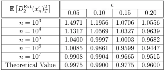
EDExt2 (xn)2T

0.05 0.10 0.15 0.20 n= 103 1.4971 1.1956 1.0706 1.0556 n= 104 1.1317 1.0569 1.0327 0.9639 n= 105 1.0400 0.9997 1.0003 0.9682 n= 106 1.0085 0.9861 0.9599 0.9447 n= 107 0.9908 0.9904 0.9665 0.9515 Theoretical Value 0.9975 0.9900 0.9775 0.9600

Table 4.1: Expectation of the (ExtQV) for dierentn's and's and for σ= 1.

Table 4.1 presents the values of the expectation of the (ExtQV) for four dierent values of= (0.05,0.10,0.15,0.20), ve values ofn= 103,104,105,106,107and for σ= 1. The last line of the table corresponds to the theoretical value of the (ExtQV) asn→ ∞ which is given by

lim n→∞E

DExt₂ (x_n)2_T=σ2

1 +2

1−e−1/2

.

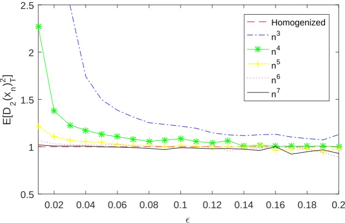
Figure 4.1 presents the value of the expectation of the (ExtQV) for a range of values in the interval[0.01,0.20]and the ve values ofn. This gure emphasizes the fact that a sucient large of sample sizenshould be considered in order the quantity

1

n2 <<1. This ensures that the error due to the discretization is negligible. Indeed, we observe that the smaller the value ofis, the larger the sample size should be in order for the (ExtQV) to perform as expected. For example, considering both Table 4.1 and Figure 4.1, when =0.20 the (ExtQV) converges much faster to the expected value than for= 0.05.

0.02 0.04 0.06 0.08 0.1 0.12 0.14 0.16 0.18 0.2

0

0.5 1 1.5 2 2.5

E[D

2

(x n ) T 2 ]

Homogenized

n3

n4

n5

n6

n7

Figure 4.1: Expectation of the (ExtQV) for dierent n's and's and for σ= 1.

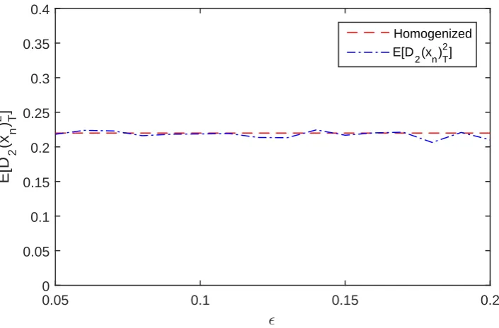
show the behavior of the (ExtQV) with respect to the scale separation parameter for σ = 1 and σ = 2, respectively. For a sucient large sample size of our data (in this casen= 106), as the value of separation parameter is getting smaller then the expectation of the (ExtQV) is getting closer to the square of the homogenized diusion coecient. For this reason in Figure 4.2 is going to 1 and in Figure 4.3 is going to 4.

Finally, in Figure 4.4, we xand nand we examine the behavior of our estimator for dierent values of σ. The heuristics in Figure 4.4 suggest that the expectation of the (ExtQV) achieves the value of the homogenized coecient for any value ofσ.

4.3.2 Consistency of the Extrema Quadratic Variation

The consistency of the (ExtQV) is examined via theL2error, i.e.

E

E DExt2 (xn)T 2

−σ22

.

0.02 0.04 0.06 0.08 0.1 0.12 0.14 0.16 0.18 0.2

0

0.5 1 1.5

E[D

2

(x

n

) T 2 ]

Homogenized

E[D 2(xn)T

2_]

<2 (1-02 (1-e-(1/0

2 )

))

Figure 4.2: Expectation of the (ExtQV) for dierent 's and for xed n= 106 and σ= 1.

0.02 0.04 0.06 0.08 0.1 0.12 0.14 0.16 0.18 0.2

0

2.5 3 3.5 4 4.5 5 5.5

E[D

2

(x n ) T

2 ]

Homogenized

E[D 2(xn)T

2 ]

<2 (1-02 (1-e-(1/0

2 )

))

0 0.5 1 1.5 2 2.5 3 3.5 4

<2

0 0.5 1 1.5 2 2.5 3 3.5 4

E

[

D2

(

xn

)

2 ]T

<2

E[D 2(xn)T

2 ]

Figure 4.4: Expectation of the (ExtQV) for dierentσ's and for xed n= 106 and = 0.10.

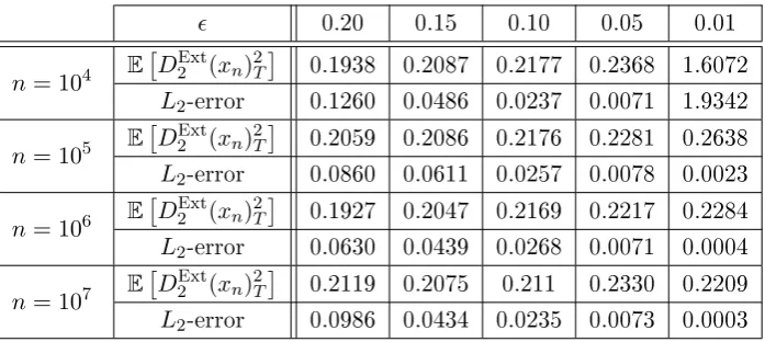
E h

DExt₂ (x_n)2_T −σ22i

0.05 0.10 0.15 0.20 n= 103 0.2985 0.1785 0.1792 0.3638 n= 104 0.0476 0.1250 0.2650 0.3548 n= 105 0.0306 0.1154 0.2380 0.3800 n= 106 0.0273 0.10 0.1986 0.3874 n= 107 0.0261 0.1008 0.1992 0.3824

Table 4.2: L2error of the (ExtQV) for dierentn's and's and for σ= 1.

estimator performs with anL2error of order2.

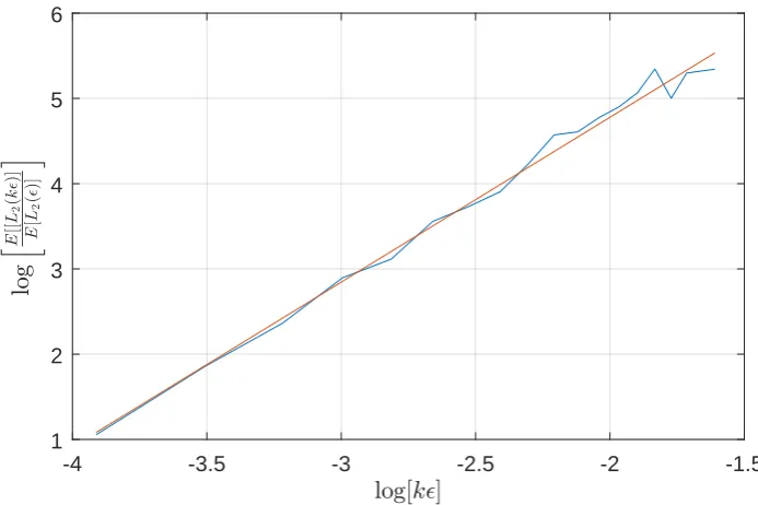
Figure 4.5 represents the loglog plot between the ratio of theL2error corresponding tokand theL2error corresponding towith respect tolog(k)wherek= 1, . . . ,20. The behavior of the loglog plot is linear with slop roughly equal to 2 (red line). For example this means that theL2 corresponding to 2= 0.02 is 4 times the L2error corresponding totimes a quantity of order2 (for this example 42).

4.4 Summary

-4 -3.5 -3 -2.5 -2 -1.5

log[k0]

1 2 3 4 5 6

lo

g

h E

[[

L2

(

k

0

)]

E

[

L2

(

0

)]

i

Figure 4.5: Loglog plot between the ration of theL2error corresponding tokand

L2error corresponding towith respect to log(k).

CHAPTER

5

General Bounded Variation Model

The objective of this chapter is to examine if the proposed estimator can be used for more general models with zero quadratic variation. We start by introducing the general form of the multiscale models that will be considered in this chapter. Then, the analytical proof that the (ExtQV) is asymptotically unbiased for this class of models is presented. Finally, we extend our results when the corresponding homogenized diusion contains also a drift term.

5.1 The General Model

In the general case, fast/slow systems of SDEs of the following form are considered

dx(t) = 1 f(y

_{(t))dt, x(0) =x}

0, (5.1a)

dy(t) = 1 2g(y

_(t))dt+β(y)

dV(t), y

_{(0) =y}

0, (5.1b)

where (x, y) ∈ X × Y = T×T, (T is the unit torus) V is the standard one

dimensional Browinan motion and the functionsf,g andβ and all their derivatives are continuous, smooth and uniformly bounded on the torus. Under these assump-tion the generator of they process,L0, is a bounded operator with respect to the

L∞ norm on the torus. Furthermore, we assume that its inverse, L−1₀ , exist and is also bounded with respect to theL∞ norm.

the processX solving the following SDE

dX(t) =σdW(t), X(0) =x0, (5.2)

whereW is the standard Brownian motion and is independent of V. The diusion coecientσ, which for this class of models is constant, is given by

σ2 = 2 ˆ

Y

f(y)Φ(y)ρ∞(y)dy = 2Ey[f(y)Φ(y)], (5.3)

where the expectation is with respect to the invariant density of they process. The functionΦ(·) solves the Poisson problem

(L₀Φ) (y) = −f(y), ˆ

Y

Φ(y)ρ∞(y)dy = 0, (5.4)

Φ(y) is periodic on Y.

Remark 5.1. Since y is a Markov process, its corresponding generator, L0, is a second order elliptic operator and Backward Kolmogorov Equation (BKE) becomes an initial value problem for parabolic PDEs (see Pavliotis (2014)).

By Fredholm alternative for elliptic PDEs with periodic boundary conditions, Eq.(5.4) has a unique centered solution, see Pavliotis and Stuart (2008, Chapter 6).

Remark 5.2 (Lemma 18.3 in Pavliotis and Stuart (2008)). The function Φ and all its derivatives are smooth and uniformly bounded.

A necessary assumption for the multiscale model (5.1) to produce a sensible limit as →0is the Assumption 2.5, i.e.

ˆ

Y

f(y)ρ∞(y)dy= 0. (5.5)

Notice that for this particular model, the homogenized SDE (5.2) does not contain a drift coecient. Indeed, from Eq.(2.11) the drift of the homogenized SDE is given by

F(X) = ˆ

Y

f1(x, y)ρ∞(y;x)dy= 0

Similar to Chapter 4, the objective of this chapter is to show that the (ExtQV) for data from models of the form (5.1) is asymptotically unbiased for the diusion coecient of the limiting diusion process. This result is summarized in the Theorem 5.3.

Before we proceed to the statement of our main result we should dene x_n the approximation ofx on a partitionπn([0, T]) :={t0, . . . tn},ti :=iδ.

Theorem 5.3. Let x(t) : [0, T] → R be a realvalued path described by Eq.(5.1).

Then, subject to technical assumptions on the behavior of the functions f, g and β (given in Assumption 5.5 on page 50), as → 0 the square of the (ExtQV) is asymptotically unbiased for σ2 in Eq.(5.2), i.e.

lim →0nlim→∞E

h

DExt₂ (x_n)T 2i

= 2E[f(y)Φ(y)]. (5.6)

Steps of the proof. 1. As in the proof of the simple model in Chapter 4 and since the model of interest is again of bounded variation the expectation of the (ExtQV) can be obtained by computing the following expression

4 n X

k=2

(n+ 1−k)E∆xn(t1)∆xn(tk)1C cx

1,k

, (5.7)

whereC,cx_1,k and 1C cx

1,k

as before (see p.22).

2. Express the increments of the process x in terms of f(y(t0)) and Φ(y(t0)) and show that

4 n X

k=2

(n+ 1−k)E∆xn(t1)∆xn(tk)1C cx

1,k

−2E[f(y(t0))Φ(y(t0))]

→0,

(5.8) asn→ ∞ and→0.

5.2 Analytical Proof of Theorem 5.3

In Lemma C.2 we have shown that by applying ItôTaylor expansion on f(y) (see Kloeden and Platen (1999, Chapter 5)) we get the following approximation forf

f(y_n(t)) =e

(t−_ti−1)

2 L0f(y_n(t_i−1)) +1

ˆ t

ti−1

e(t −u)

2 L0(∇_y

nf β)(y

Given Eq.(5.9) we obtain the following expression for the increments of the process x_n

∆x_n(ti) = 1

ˆ ti

ti−1

f(y_n(t))dt

=eδ2L0 −1

L−1₀ f(y_n(ti−1))

+ 1 2

ˆ ti

ti−1

ˆ t

ti−1

e

(t−u)

2 L0_(∇

y

nf β)(y

n(u))dV(u)dt. (5.10)

The justication of Eq.(5.10) can be found in Lemma C.3.

At this point, we have extracted an expression for the increments of the processx_n similar to the one in Eq.(4.11) for the OrnsteinUhlenbeck case. To simplify our computations, lets dene

ψ(y_n(ti)) :=

eδ2L0−1

L−1₀ f(y_n(ti−1)), (5.11)

and

Mti := 1 2

ˆ ti

ti−1

ˆ t

ti−1

e(t −u)

2 L0(∇_y

nf β)(y(u))dV(u)dt. (5.12)

Therefore, given the notation in equations (5.11) and (5.12), the product of our interest, ∆x_n(t1)∆xn(tk), takes the following form

∆x_n(t1)∆xn(tk) =ψ(yn(t0))ψ(yn(tk−1)) +Mt1Mtk

+ψ(y_n(tk−1))Mt1+ψ(y

n(t0))Mtk, (5.13)

and the expectation in Eq.(5.7) becomes

E h

∆x_n(t1)∆xn(tk)1C

cxn

1,k i

=Eψ(yn(t0))ψ(yn(tk−1))1C ψ(y_n) +M

(5.14a)

+EMt1Mtk1C ψ(y

n) +M

(5.14b) +Eψ(yn(tk−1))Mt11C ψ(y

n) +M

(5.14c) +Eψ(yn(t0))Mtk1C ψ(y

n) +M

,

(5.14d)

Our aim is to prove that 4 n X k=2

(n+ 1−k)E h

∆x_n(t1)∆xn(tk)1C

cxn

1,k i

−2E[f(yn(t0)) Φ (yn(t0))]

| {z }

:=E

→ 0,

(5.15)

asn→ ∞ and→0, or equivalently from Eq.(5.14),

4 n X k=2

(n+ 1−k) [(5.14a)+(5.14b)+(5.14c)+ (5.14d)]

−2E[f(yn(t0)) Φ (yn(t0))]

→0. (5.16)

But, from triangular inequality we get

E ≤ 4 n X k=2

(n+ 1−k) [(5.14a)]−2E[f(yn(t0)) Φ (yn(t0))] + 4 n X k=2

(n+ 1−k) [(5.14b)]

+ 4 n X k=2

(n+ 1−k) [(5.14c)]

+ 4 n X k=2

(n+ 1−k) [(5.14d)]

. (5.17)

In what follows, we initially prove that the second, third and fourth term in Eq.(5.17) tend to zero as n → ∞ and later that the rst term tend to zero as n → ∞ and →0.

Starting from the second term, applying consequently Jensen's, CauchySchwarz inequality and the fact that1C ψ y_n+M≤1we get

4 n X k=2

(n+ 1−k) [(5.14b)]

= 4 n X k=2

(n+ 1−k)EMt1Mtk1C ψ y

n +M ≤ 4 n X k=2

(n+ 1−k)E[|Mt1Mtk|]

≤ 4 n X

k=2

(n+ 1−k)EMt21

1/2

EMt2k

1/2

≤ 4C 7

n X

k=2

asn→ ∞ where the latter inequality comes from the result in Lemma C.4.

For the third term, to further simplify our computations, notice that

ψ(y) = eδ2L0_L−1

0 f(y)−L−10 f(y)

= ∞ X m=0 δ 2 m

L(₀m)L−1₀ f(y)

m! −L

−1 0 f(y)

= δ f(y

_{) +} ∞ X m=2 δ 2 m

L(₀m)L−1₀ f(y₎

m!

= δ f(y

₎₋ ∞ X m=2 δ 2

m_L(m) 0 Φ(y)

m!

| {z }

:=λ(y)

. (5.18)

Using the latter expression forψ(y)and the same arguments with the previous term we obtain 4 n X k=2

(n+ 1−k) [(5.14c)]

= 4 n X k=2

(n+ 1−k)E

δ f(y

n(t0))−λ(yn(t0))

×Mtk1C ψ y

n +M ≤ 4 n X k=2

(n+ 1−k) n E[f(y

n(t0))Mtk×

1C ψ y_n +M (5.19a) + 4 n X k=2

(n+ 1−k)E[λ(yn(t0))Mtk×

1C ψ y_n+M

. (5.19b)

We treat each of the terms in Eq.(5.19a) and Eq.(5.19b) separately. For Eq.(5.19a), following the same approach as before we get

Eq.(5.19a) ≤ C n X

k=2

(n+ 1−k)

n E

f(y_n(t0))2 1/2

EMt2k

1/2

.

whereC is a constant depending only on . Our assumptions on f and the result