Please cite this paper as:
Schaer, O., Kourentzes, N. and Fildes, R. 2018. Demand forecasting with user-generated online information. Lancaster University Management School, Management Science Working Paper 2018:2, 1-41.
Managmeent Science
Working Paper 2018:2
Demand forecasting with user-generated
online information
Oliver Schaer, Nikolaos Kourentzes and Robert Fildes
The Department of Management Science
Lancaster University Management School
Lancaster LA1 4YX
UK
© Oliver Schaer, Nikolaos Kourentzes and Robert Fildes All rights reserved. Short sections of text, not to exceed two paragraphs, may be quoted without explicit permission,
Demand forecasting with user-generated online information
Oliver Schaera,∗, Nikolaos Kourentzesa, Robert Fildesa
aDepartment of Management Science, Lancaster University Management School, UK
Abstract
Recently, there has been substantial research on augmenting aggregate forecasts with individual consumer data from internet platforms, such as search traffic or social network shares. Although the majority of studies report increased accu-racy, many exhibit design weaknesses including lack of adequate benchmarks or rigorous evaluation. Furthermore, their usefulness over the product life-cycle has not been investigated, which may change, as initially, consumers may search for pre-purchase information, but later for after-sales support. In this study, we first review the relevant literature and then attempt to support the key findings using two forecasting case studies. Our findings are in stark contrast to the literature, and we find that established univariate forecasting benchmarks, such as expo-nential smoothing, consistently perform better than when online information is included. Our research underlines the need for thorough forecast evaluation and argues that online platform data may be of limited use for supporting operational decisions.
Keywords: Google Trends, Social media, Leading indicators, Product life-cycle, search traffic, electronic word-of-mouth
1. Introduction
Nowadays it is becoming increasingly easy for organisations to obtain
indi-vidual consumer behaviour data from potential and actual customers by using
internet platforms, such as Google or Twitter. Consumers seek online information
on branded and non-branded content (Heinonen, 2011). Companies actively
sup-port purchase decisions by distributing branded content through internet channels,
∗Correspondance: O Schaer, Department of Management Science, Lancaster University
Man-agement School, Lancaster, Lancashire, LA1 4YX, UK. Tel.: +44 1524 592911
Email addresses: [email protected] (Oliver Schaer),
which generates further interactions (Kuksov et al., 2013; Wang et al., 2012).
Re-search has argued that information such as Re-search traffic popularity, or numbers of
shares on social networks can lead to improved forecast accuracy (e.g. Cui et al.,
2017; Geva et al., 2017; Goel et al., 2010). While online shares reflect an electronic
word-of-mouth process (Seiler et al., 2017; Babic Rosario et al., 2016), the popu-larity of a search keyword can be regarded as a proxy for consumer interest in a
product (Du and Kamakura, 2012; Stephen and Galak, 2012), but also reflect the
success of advertising activities (Srinivasan et al., 2016; Hu et al., 2014).
There are numerous time series modelling papers that incorporate information
from the internet; for instance, in econometric now-casting such inputs can be
useful to overcome publication lags of governmental economic indicators or market
surveys (e.g. Vosen and Schmidt, 2011; Choi and Varian, 2009). Other example
include predicting stock volatility (e.g. Bollen et al., 2011); infleunza outbreaks
(e.g. Ginsberg et al., 2009); tourist arrivals (e.g. Hand and Judge, 2012); car sales
(e.g. Fantazzini and Toktamysova, 2015; Du et al., 2015); and retail sales (e.g. Boone et al., 2018; See-To and Ngai, 2016).
One important aspect is that most business decisions, such as allocating
re-sources, inventory decisions or planning marketing expenditures, are based on
forecasts and in turn imply some forecast lead time, which is relevant for the
deci-sion planning horizon. This makes the usefulness of online information for demand
forecasting more contentious. Past research has supported both its usefulness (e.g.
Lau et al., 2017; Brynjolfsson et al., 2016; Schneider and Gupta, 2016) and its
lim-itations (e.g. Ruohonen and Hyrynsalmi, 2017; Li, 2016; Limnios and You, 2016).
A further complication in assessing the value of such inputs for operational deci-sion making comes from the typically weak forecast evaluation setup that is used
and the short forecast horizons, which often do not relate realistically to
busi-ness needs. Kalampokis et al. (2013) in their review of forecasting with social
media data, report that more than one-third of studies do not test the claimed
predictive abilities, using hold-out-sample or adequate predictive measures. Their
review does not consider research that includes information originating from other
than social media networks, for example, search traffic information; and omits any
dedicated discussion on the forecasting approaches used.
liter-ature on forecasting with internet-based consumer behavioural data for a range
of applications; (ii) discuss the limitations and challenges of using such data for
predictive purposes and (iii) explore whether the usefulness of such information
remains consistent during a product’s life-cycle. To exemplify this, consider a
consumer who may research a product online prior to purchasing. The search is a leading indicator. Post-purchase the same consumer may search online for support
information that does not lead to additional purchases. Therefore, it is reasonable
to expect that the usefulness of online information changes over the life-cycle of
a product. To support our critical review of the literature, first, we replicate one
experiment by Choi and Varian (2012) and second, we model sales of video games
and the consumption of viral video advertisements using social network shares.
Although the literature is overwhelmingly positive as to the benefits of search
traffic and social media derived variables, we argue otherwise given the evaluation
and experimental design of almost all studies. We question the realism of the
forecasting setup (for instance the forecast horizon) for a number of papers and also find that several do not include adequate benchmarks. Furthermore, we find
no support where the usefulness of the variable changes over the life-cycle of a
product from our empirical experiment.
The paper is organised as follows; Section 2 provides a review of the literature
that uses explanatory variables from internet platforms for forecasting. Section 3
highlights the challenges in handling online information. We then present in
Sec-tion 4, two case studies to validate the findings of the literature. SecSec-tion 5 discusses
the usability of internet platform information and Section 6 presents the
conclu-sions.
2. Forecasting with online user generated data
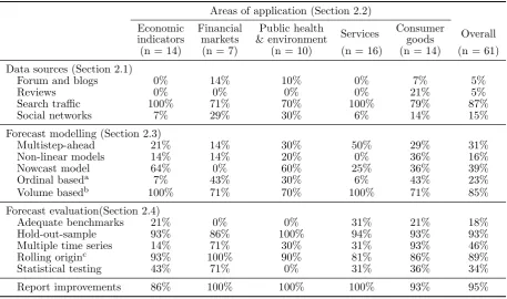
We present the literature in four subsections which are summarised in Table 1.
The first horizontal grouping summarises Section 2.1, which surveys data sources. The columns reflect groups of forecast applications, which are detailed in Section
2.2. The second horizontal grouping classifies the forecast models used and is
discussed further in Section 2.3. The last grouping lists forecasting principles, to
conclude in favour of using user-generated information for forecasting. A detailed
table for each area of application is provided in the online supplement of this paper.
We limit our literature review to studies that assess the forecasting
perfor-mance of time series models on relative short horizons, relevant to operational
business forecasting. This precludes areas such as: predicting election outcomes (e.g. Mavragani and Tsagarakis, 2016; Huberty, 2015), product rankings (e.g. Hou
et al., 2017; Liu et al., 2016; Goel et al., 2010), pre-launch forecasts (e.g. Kim
et al., 2015; Xiong and Bharadwaj, 2014; Dellarocas et al., 2007) and marketing
effectiveness (e.g. Kumar et al., 2016; Hu et al., 2014; Du and Kamakura, 2012).
Although most of these studies suggest benefits from online user-generated data,
their modelling approach as well the forecast target and accuracy measures used,
differ substantially and would require a separate discussion that is out of scope for
this paper. We do, however, include some of their findings on the handling of such
[image:5.595.90.548.380.650.2]data to support our discussion.
Table 1: Summary of the literature
Areas of application (Section 2.2) Economic Financial Public health
Services Consumer Overall indicators markets & environment goods
(n = 14) (n = 7) (n = 10) (n = 16) (n = 14) (n = 61) Data sources (Section 2.1)
Forum and blogs 0% 14% 10% 0% 7% 5% Reviews 0% 0% 0% 0% 21% 5% Search traffic 100% 71% 70% 100% 79% 87% Social networks 7% 29% 30% 6% 14% 15% Forecast modelling (Section 2.3)
Multistep-ahead 21% 14% 30% 50% 29% 31% Non-linear models 14% 14% 20% 0% 36% 16% Nowcast model 64% 0% 60% 25% 36% 39% Ordinal baseda 7% 43% 30% 6% 43% 23%
Volume basedb 100% 71% 70% 100% 71% 85%
Forecast evaluation(Section 2.4)
Adequate benchmarks 21% 0% 0% 31% 21% 18% Hold-out-sample 93% 86% 100% 94% 93% 93% Multiple time series 14% 71% 30% 31% 93% 46% Rolling originc 93% 100% 90% 81% 86% 89% Statistical testing 43% 71% 0% 31% 36% 34% Report improvements 86% 100% 100% 100% 93% 95%
2.1. Data sources
Two review papers have been published that cover forecasting with social media
networks (Phillips et al., 2017; Kalampokis et al., 2013). This study considers a
wider range of internet sources for obtaining user-generated information. These are
search traffic, social network sites, blogs and microblogs, forum posts and online
product reviews. We do not specifically include studies which obtain data from
news streams, such as the GDELT project (e.g., Fast et al., 2017), because such
information may not reflect online consumer behaviour. It is worthwhile noting
that we were unable to find any research that explores the predictive ability of
many popular social media platforms such as Instagram, Snapchat, Pinterest and LinkedIn. The same is true for user-generated videos from platforms like YouTube,
even though studies suggest that video blogs can lead to positive purchase intention
(Lee and Watkins, 2016). The limited use of these data sources might partly be
due to the difficulty to access and identify content.
Search traffic information is the most frequently used source present in 87%
of the investigated studies, even accounting for 100% of applications in economics
and services. Search engines tend to have a better coverage of the population
and topics of past research, such as unemployment, are unlikely to be shared
on social networks (D’Amuri and Marcucci, 2017). Most studies use data from Google Trends and fewer from Naver (Jun et al., 2017; Kim and Shin, 2016) or
Baidu (Huang et al., 2017; Li et al., 2017) that are popular search engines in South
Korea and China, respectively.
Microblogging platforms, such as Twitter (e.g. Bughin, 2015; Skodda and
Ben-thaus, 2015; Rao and Srivastava, 2013) and Weibo (Chen et al., 2017) are the
second most popular type of data source. The only study which involves social
network sites is by Cui et al. (2017), who use Facebook. Bughin (2015) obtains
social media information from SocialMention, a free aggregation service
cover-ing various platforms includcover-ing Reddit. Another source is product reviews that have been collected from sources such as Amazon (Schneider and Gupta, 2016)
or CNET (Luo and Zhang, 2013). Furthermore, Google search has been used to
2.2. Forecasting applications
A typical application in economics is to forecast unemployment rate and claims.
While various researcher report positive results (e.g. D’Amuri and Marcucci, 2017;
Smith, 2016; Barreira et al., 2013) others struggle to improve accuracy (Li, 2016;
Choi and Varian, 2012). Brynjolfsson et al. (2016) report benefits by stressing
the importance of keyword selection. Researchers also look into housing market
(Limnios and You, 2016; Wu and Brynjolfsson, 2015; Choi and Varian, 2009),
private consumption (Vosen and Schmidt, 2011), exchange rates (Bulut, 2017),
commodities (Yu et al., 2018; Elshendy et al., 2017) as well as consumer sentiment
and gun sales (Scott and Varian, 2015). All but Limnios and You (2016) report improvements.
Financial applications include the predictions of financial market indices (Bollen
et al., 2011), their returns (Perlin et al., 2017) or volatility (Dimpfl and Jank, 2016;
Hamid and Heiden, 2015). Rao and Srivastava (2013) investigate stock market
in-dexes but also currency exchange rate and gold prices. Other researchers forecast
stock returns (Ho et al., 2017; Bijl et al., 2016). All studies report forecast
im-provements and Perlin et al. (2017) find search traffic to be particularly useful
during the financial crisis.
When considering service-oriented applications, a large number of studies find improved forecast accuracy for tourism destinations (Li et al., 2017; Padhi and
Pati, 2017; Park et al., 2017; Zeynalov, 2017; Choi and Varian, 2009) and
attrac-tions (Huang et al., 2017; Peng et al., 2016). In the case of Bangwayo-Skeete and
Skeete (2015) search traffic outperforms the univariate benchmark only for
one-third of the examined tourist destinations. Nonetheless, the authors conclude in
favour of using this information, as in 77% of the cases accuracy was better or at
least as good as the benchmarks. ¨Onder (2017) did not find any clear indication
whether search traffic is performing better on city or country level since. Her study
reports improvements for both categories, but in several cases the benchmark is not outperformed ( ¨Onder and Gunter, 2016, report similar findings). Rivera (2016)
reports that the benchmark is outperformed for 12 month ahead forecasts, but not
for shorter ones. For hotel room demand forecasting, Pan et al. (2012) improve
accuracy, but in a different study Pan and Yang (2016) find no statistically
applications include Telecom contract sales (Bughin, 2015) or the number of air
passengers (Kim and Shin, 2016).
A majority of studies that focus on consumer goods, forecast on aggregated
brand or product category level. For example, Cui et al. (2017) report
improve-ments for fashion sales forecast using sentiment information. Various studies also investigate car sales. Researchers find improvements from either search traffic
(Carri`ere-Swallow and Labb´e, 2013; Seebach et al., 2011) or forum posts (Geva
et al., 2017). Fantazzini and Toktamysova (2015) report search traffic to be
par-ticularly helpful at longer forecast horizons. However, Choi and Varian (2009)
report mixed findings and Choi and Varian (2012) as well as Barreira et al. (2013)
conclude that there is little support for including search traffic. Also, the search
traffic augmented model of Jun et al. (2017) which forecasts global netbook sales
fails to outperform the benchmark. They also fail to improve forecast accuracy for
Nintendo Wii sales, indicating that forecasting at product level is more
challeng-ing. Geva et al. (2017) for instance report increased errors due to additional noise in the data. Nevertheless, several studies report accuracy gains even at product
level for speciality food Stock Keeping Units (SKUs) with search traffic (Boone
et al., 2018, 2015), but also with sentiment information for electronic products
(Lau et al., 2017; Schneider and Gupta, 2016) or fashion products (See-To and
Ngai, 2016).
In the area of public health, various studies have been concerned with flu
outbreaks. Ginsberg et al. (2009) incorporate highly correlated search terms to
predict the flu index which became the Google Flu indicator. Its service was
discontinued in 2015, partly because of data reliability concerns (Lazer et al., 2014; Butler, 2013). Despite the critique of Google Flu, studies find the combination of
Google Trends and autoregressive terms leads to better results (Lazer et al., 2014;
Preis and Moat, 2014). Moreover, with further refinement of keyword selection,
there are additional improvements (Brynjolfsson et al., 2016). Influenza outbreaks
are also successfully forecasted with information from Twitter and blogs (Santillana
et al., 2015; Won et al., 2013; Lampos and Cristianini, 2012).
Studies that focus on environmental events are sparse and online user-generated
information is mainly used for posthoc analysis. Examples of usage are Lampos
(2017) that predict smog hazards. Both use information from microblogs. It is
worth noting that we were unable to identify studies that consider energy demand
as an application, even though this is closely related to local weather conditions.
2.3. Forecast modelling
The majority of studies use linear regression models (Schneider and Gupta,
2016; Ginsberg et al., 2009), augmented with autoregressive terms (e.g Peng et al.,
2016; Barreira et al., 2013; Seebach et al., 2011) and moving average terms (e.g. Li
et al., 2017; Padhi and Pati, 2017; Pan and Yang, 2016). Linear vector models are
also applied successfully (e.g Dimpfl and Jank, 2016; Fantazzini and Toktamysova, 2015). Other options include Bayesian structural models (Scott and Varian, 2015),
dynamic linear models (Rivera, 2016) and Seemingly Unrelated Regression (Ho
et al., 2017). Models that use the higher frequency of online information are also
considered, e.g. Mixed-Data Sampling (Zeynalov, 2017; Smith, 2016;
Bangwayo-Skeete and Bangwayo-Skeete, 2015); or Dynamic Factor Models with mixed frequencies (Li,
2016).
Machine learning methods, typically incorporating sentiment information from
social networks and review data (including mentions in forums), are also
com-mon. These include AdaBoost (Santillana et al., 2015), Support Vector Machines (Yu et al., 2018; Chen et al., 2017; Cui et al., 2017; Schneider and Gupta, 2016;
Santillana et al., 2015), Random Forests (Cui et al., 2017) and Neural Networks
(Yu et al., 2018; Chen et al., 2017; Lau et al., 2017; Geva et al., 2017; Bollen
et al., 2011). These provide evidence of non-linearities in the relationships (e.g.
Lau et al., 2017; Geva et al., 2017).
The majority of economic indicators are modelled with nowcasting models that
include a contemporaneous internet variable to overcome the publication lag
(ex-cept D’Amuri and Marcucci, 2017; Limnios and You, 2016; Barreira et al., 2013).
Such models are also popular for forecasting influenza outbreaks (Xu et al., 2017; Preis and Moat, 2014; Ginsberg et al., 2009). However, some studies use
nowcast-ing to forecast target variables in an operational context, which raises questions
as to their usefulness due to the required lead times: for example, visitor
ar-rivals (Huang et al., 2017; Zeynalov, 2017; Choi and Varian, 2009), Telecom sales
2013; Choi and Varian, 2009) and fashion sales (See-To and Ngai, 2016). There
are also studies which are not framed as nowcasting, but include contemporaneous
inputs (Chen et al., 2017; Jun et al., 2017; ¨Onder, 2017; Schneider and Gupta,
2016; Boone et al., 2015).
A key aspect of the model building is the specification of the user-generated information variables. The data is incorporated directly in the case of search
traf-fic and count data, such as search popularity, the number of mentions or shares.
Note that Google Trends and Naver provide peak scaled indexes, where different
keywords compare relatively to each other (see Jun et al., 2017). Baidu, on the
other hand, provides absolute search values (see Vaughan and Chen, 2015). Other
inputs are ordinal such as product ratings (Schneider and Gupta, 2016) or
sen-timent information. See-To and Ngai (2016) incorporate sensen-timent information
in the form of the absolute number of positive and negative reviews per period,
whereas others use the ratio of positive and negative mentions per period (e.g.
Geva et al., 2017; Skodda and Benthaus, 2015). If content-based information is available, it is also important to take into account the rating for the comment
itself, i.e. by weighting up-votes for helpful reviews (Schneider and Gupta, 2016).
Although several studies find sentiment to provide additional benefits over volume
based information (Lau et al., 2017; Geva et al., 2017; Bughin, 2015), such gains
are still debatable, given the additional complexity. K¨ubler et al. (2017) indicate
that the required method, as well as choice of metrics, depend on brand strength
and industry segment. We discuss keyword selection and sentiment measure in
more detail in Sections 3.3 and 3.4.
2.4. Forecast evaluation
The forecasting literature has established several forecasting principles that
make the interpretation and comparison of forecasts more transparent. These
include the need for adequate benchmarks (Armstrong, 2006; Armstrong and Col-lopy, 1992) and hold-out sample evaluation with rolling origins (Tashman, 2000).
The selected error metrics should be conditional on the forecasting objective and
a number of alternatives should usually be included as the result maybe
contra-dictory (Davydenko and Fildes, 2013; Fildes and Ord, 2002). For example using
(2005) also stress the importance of statistically testing the performance of
com-peting models. The surveyed literature adherence to these practices in a mixed
manner, as Table 1 depicts.
There are issues about the clarity of the experimental setup. For example, Yu
et al. (2018), Araz et al. (2014) and Won et al. (2013) provide very little details about the model specifications of user-generated variables. Various studies are also
unclear on the set up of the evaluation sample (Chen et al., 2017; Jun et al., 2017; ¨
Onder, 2017; Choi and Varian, 2009). Although, most studies use hold-out samples
with rolling origins some of the studies evaluate them on very few observations
(Elshendy et al., 2017; Araz et al., 2014). Other studies do not report extensive
forecast results, which makes it difficult to identify any performance improvements
(Bangwayo-Skeete and Skeete, 2015; Carri`ere-Swallow and Labb´e, 2013).
If claims are to be made about the generalisability of the results, multiple time
series should be used. As the online supplement attests, less than half of the
investigated literature report results for multiple series, and some of the remaining studies do not investigate more than two series (e.g. Rao and Srivastava, 2013;
Seebach et al., 2011). However, in some cases carrying out experiments for multiple
time series is not possible for applications that focus on highly aggregated variables.
Nonetheless, these could, for example, be split into regions to provide more robust
results such as in (Bulut, 2017; ¨Onder and Gunter, 2016; Bangwayo-Skeete and
Skeete, 2015; Lampos and Cristianini, 2012). One-third of the surveyed literature
also includes statistical testing of the forecast results that typically strengthen their
findings. However, in the case of Bulut (2017) they lead to contradictory results
since none of the search traffic augmented models outperforms the random walk on the MSPE, but the test find them to be significantly better. The contradiction
maybe explained by the distribution of the forecast errors. This led the authors
to still draw a positive conclusion on the usefulness of search traffic data.
A further issue is that the conditionality of forecasts is unclear. For example,
it is unclear whether Hand and Judge (2012) use a 4 observation long test set in a
rolling origin manner or whether the horizon is set to four. The study by D’Amuri
and Marcucci (2017) provides 12-month ahead forecast, but the maximum lag
length of search traffic is four, requiring unseen future information. Several studies
known or not in the test set ( ¨Onder, 2017; ¨Onder and Gunter, 2016;
Bangwayo-Skeete and Bangwayo-Skeete, 2015; Won et al., 2013). Li et al. (2017) report significant
improvement for 4-weeks-ahead forecasts, using 5 lags of search traffic, but are
unclear if the values of the shorter lags were considered known or not. Barreira
et al. (2013) indicate that the 36 month out-of-sample forecast uses future values. Less than one-third of the surveyed studies considered multistep-ahead forecasts.
It is questionable how relevant one-step-ahead forecasts are in a business context
that for example require stock keeping (Boone et al., 2018; Lau et al., 2017; Geva
et al., 2017; See-To and Ngai, 2016; Seebach et al., 2011).
A further critique of the existing literature is that studies often fail to provide a
thorough comparison with adequate benchmarks. For example the studies by Kim
and Shin (2016); Won et al. (2013); Lampos and Cristianini (2012); Ginsberg et al.
(2009) and partly Choi and Varian (2009) report no benchmarks at all. Lau et al.
(2017); Xu et al. (2017); Peng et al. (2016); Skodda and Benthaus (2015) and Hand
and Judge (2012) only compare forecast performance amongst models that include online information. Most papers use at least one benchmark that is the univariate
equivalent of the proposed model using the additional internet variables. However,
established, and common in practice models, such as exponential smoothing or
the random walk, are often absent. If such benchmarks outperform both the
univariate and the enhanced models, then there is little value in them. Therefore,
the apparent lack of a thorough (or even valid in some cases) forecast accuracy
evaluation diminishes the value of the reported improvements.
To exemplify this, Cui et al. (2017) report gains over the company forecast,
but there is too little information on how the company forecast is produced or whether it was any good at all. This critique echoes the arguments by Li (2016),
¨
Onder (2017) and Fantazzini and Toktamysova (2015), who all report cases where
the random walk outperforms models that use search traffic information for some
evaluation periods. Jun et al. (2017) and Rivera (2016) similarly find that the
simple Holt-Winters method performs better than forecasts that used additional
internet information. In a study by Lazer et al. (2014) the Google Flu index
model is outperformed by a univariate model. A further downside of not using
established benchmarks is that it makes any meta-analysis of performance very
To further illustrate the importance of including a wide variety of benchmark
models we replicate one of the experiments conducted by Choi and Varian (2012)
and extend its range of contenders. In addition to the proposed seasonal
autore-gressive model, we further include the random walk (RW), as well as the Simple
Exponential Smoothing model (SES) and the Holt-Winter model (HW). Table 2 provides the Mean Absolute Percentage Errors (MAPE). The result suggests that
the Holt-Winters model performs best in both evaluation periods. Furthermore,
none of the models differ significantly at a 95% level when evaluated with the
[image:13.595.149.446.296.340.2]Friedman and Nemenyi tests (Demˇsar, 2006).
Table 2: MAPE for motor vehicles and parts (Choi and Varian, 2012)
AR ARX RW SES HW
06/2005 - 07/2011 6.34% 5.67% 6.88% 6.70% 4.37%
12/2007 - 06/2009 8.87% 6.97% 5.87% 5.75% 4.84%
leadtime= 1,italic signifies original models
In the introduction, we posed the question whether such predictive information
remains relevant over the life-cycle of a product or service. There is some evidence
from the marketing literature that reports the impact of social network variables
changing over time, due to changes in the level of customer engagement (Kumar et al., 2016). Smith (2016) finds changing coefficients of Google Trends indicators,
some switching from positive to negative, over the life-cycle. It is unclear whether
this indicates a spurious or changing relationship. Experiments which have
in-cluded a rolling window evaluation with re-estimation do not provide insights on
the changes of the coefficients and in particular do not discuss the life-cycle aspect
(e.g. Cui et al., 2017; Geva et al., 2017; Bughin, 2015).
2.5. Summary
To summarise the literature review we note that a majority of investigated
papers report positive findings for all types of user-generated data sources. The
most frequently applied models are linear in the form of an ARX model, both in
nowcasting and forecasting. However, the conclusions of these studies must be
tempered by their many limitations, in particular the absence of adequate
conditional on. To be useful in operational planning decisions they also need to be
focussed on a meaningful forecast horizon. Given these weaknesses in the forecast
evaluation framework, we therefore cannot conclude as to which applications are
likely to benefit from user-generated information.
3. Handling user generated online information
3.1. Data consistency and reproducibility
Reproducing the results of forecasting experiments is a major concern for
re-search (Boylan et al., 2015). Lazer et al. (2014) question how stable and reliable are
measurement sources such as Google Trends over time. For instance, changes in
the search algorithm employed by Google can disrupt the performance of predictive
models. Such changes are dependent on decisions by the search engine provider
that might be based on commercial interests. Changes in search algorithms not
only require model re-calibration, but also hinder scientific replication. Recently, Google restricted the maximum window length for weekly data to 5 years. Hence,
to obtain weekly data from 2004, stitching and re-scaling are required (Johansson,
2014, provides a tutorial with one way of combining). This increases the risk of
obtaining different values for the search traffic.1
Furthermore, Google Trends index depends on samples which are re-drawn
from day-to-day (Varian, 2017). According to Barreira et al. (2013) this sampling
instability explains some of the inconsistencies in the results of their now-casting
exercise. Carri`ere-Swallow and Labb´e (2013) report all queries within 24-hours to
be identical, but across a 50-day sample, the same query sample exhibit a standard deviation of more than 15%. Although, D’Amuri and Marcucci (2017) report that
the cross-correlation between series of different days is never below 0.99, they take
the average of 24 downloads over 12 days from two different IP’s for forecasting
unemployment rate. Li (2016) replicates one of the experiments by Choi and
Varian (2012) but achieves different out-of-sample forecasts between the original
1We were not able to find any official changelog of Google Trends but the
data and the newly obtained sample, highlighting issues of sample instability from
Google Trends that makes the replication of experiments more difficult. Li (2016)
suggests that taking multiple samples is a good solution, but it is unknown how
many samples are needed to approximate the “true” sample.
The research of Lazer et al. (2014) also points out that other platforms have similar issues. For example, a study by Ho et al. (2017) reports that they were
unable to report the number of messages prior to 2011 due to changes to the
Yahoo!Finance website. Ruths and Pfeffer (2014) raise concern that social
me-dia platforms can enforce changes in data streaming and filtering. For instance,
the additional “like”-buttons Facebook introduced to express emotions have an
unknown effect on data continuity. Although for practitioners reproducibility is a
minor concern, the reliability of the models and the need for continuous monitoring
of the specifications is of importance.
3.2. Data bias
One of the disadvantages of user-generated information is potential selection
sample bias. This bias exists on all platforms and affects search traffic,
prod-uct reviews as well as social network platforms (Brynjolfsson et al., 2016; Ruths
and Pfeffer, 2014). This is because the platforms are not accepted equally in all countries, and furthermore, not the entire population is using the platform equally
often. For example, Brynjolfsson et al. (2016) mentions the case that elderly people
might not use online technologies to search for products and services. This makes
the right choice of platform crucial in order to align with the forecast target.
Bias not only appears in the representation of the population, but also in
terms of content type. On social network platforms, such as Facebook, users tend
to share a positive image (Barash et al., 2010), and research suggests that
nega-tive feelings are more likely to be expressed on forums (Leung, 2013). Moreover,
not all customers write reviews and the reflected opinion might not represent the overall opinion of customers. Dellarocas et al. (2007) report customers with strong
positive or negative opinion are more likely to post. Moreover, reviews from early
adopters have been found to be systematically positively skewed due to potential
self-selection bias and the fact that early buyers may have different preferences
over the product lifetime (Godes and Silva, 2012; Li and Hitt, 2008) which impacts
sales (Moe and Trusov, 2011).
The often reported J-shaped distribution of online ratings (e.g. Schneider and
Gupta, 2016) can have many sources including fraud, selection bias or herding
effects (Aral, 2014). Fraud might be due to manipulation by companies and their competitors. Mayzlin et al. (2014) find evidence of fake hotels reviews on
Tri-padvisor with negative reviews by competitors, but also positive ones created by
the owners. Lee et al. (2017) shows that in the movie industry Twitter sentiment
is often positively manipulated in the pre-launch phase and drops after release
when actual viewers comment. Such manipulation may not only impact sales, but
also affect the willingness to post and, therefore, change the final product
percep-tion (Moe and Schweidel, 2012). Positively manipulated reviews lead on average
to 25% increased final ratings, suggesting an asymmetric herding bias (Muchnik
et al., 2013).
Although, these biases are well studied, very little is done to address them in forecast models. Nonetheless, cleansing data post-hoc, might eliminate important
signals, since a manipulated negative review that is still online will potentially
affect sales and future reviews. Even if it were removed, it is hard to track how it
has affected other remaining reviews.
3.3. Keyword selection
One of the major complication of using search traffic information is to select
keywords (Goel et al., 2010). That keyword selection matter is demonstrated in the
research by Brynjolfsson et al. (2016) discussed before. Geva et al. (2017) describes
keyword selection to be a trade-off between accuracy and coverage. Studies that tried to incorporate a very high coverage (Scott and Varian, 2015; Ginsberg et al.,
2009) base their selection to identifying keywords with the highest correlation from
very large datasets (using Google Correlate one can find correlated search queries to any given time series). While this method effectively filters amongst million of
possible queries, it remains prone to return spurious correlated time series (Lazer
et al., 2014) and requires a well-designed forecast evaluation to prevent over-fitting.
It also introduces major variable selection challenges due to the number of
A large part of the investigated literature uses a judgemental selection based on
only a few keywords, such as product or brand name (e.g. D’Amuri and Marcucci,
2017; Geva et al., 2017; Seebach et al., 2011) or words like “dow” for Dow Jones
Index (e.g. Dimpfl and Jank, 2016; Hamid and Heiden, 2015). Other studies use
more descriptive keywords for example “Gifts for colleagues” to predict a wine and cheese SKU (Boone et al., 2018) or “Vacation” to reflect economic income (Bulut,
2017). While this approach allows a better interpretation of variables selected it
might miss out important information. To broaden the numbers of keywords Li
et al. (2017) and Peng et al. (2016) use a seeding technique. They initially define
a range of keywords that was then used in a second step to gather recommended
keywords by the search engine. Perlin et al. (2017) count the frequency from a
large list of financial specific words in academic books to derive from a list of 15
se-lected words. Similarly, Padhi and Pati (2017) identify 63 keywords from different
literature sources and interviews with destination clients. Researchers also tried
to identify specific keywords to obtain pre-purchase searches only. Von Graevenitz et al. (2016) for instance use scrappage subsidies searches as pre-purchase
indi-cators of new car purchases. Hu et al. (2014) use composite search queries that
excluded unrelated search keywords for new car sales such as “repair”. Siliverstovs
and Wochner (2018) use Google Knowledge Graph that covers linguistic and
se-mantic related keywords to a topic. For example, it can combine search queries
for a place covering different languages.
Another approach is to use automatic generated categories that search
en-gines provide. These categories cover several related keywords for areas like travel
destinations or industry sectors (e.g. Von Graevenitz et al., 2016; Bughin, 2015; Fantazzini and Toktamysova, 2015; Scott and Varian, 2015; Wu and Brynjolfsson,
2015; Vosen and Schmidt, 2011; Choi and Varian, 2012). Brynjolfsson et al. (2016)
criticise such categories being opaque and might include irrelevant keywords that
could harm the predictive ability. Instead, they suggest a crowd-sourcing approach.
They asked more than 500 persons to write down five terms that came to their
mind when seeing a particular word. Not only did they achieve higher forecast
accuracy, but they also found that the forecast accuracy improves steadily when
increasing the number of selected variables (up to 20). This result is in contrast
performance decreases when additional variables are added, indicating poor
selec-tion in these cases. Although crowd-sourcing via services such as Amazon Turks
might be relatively cheap, it can quickly become expensive if keywords for several
hundreds of products are required.
Another approach is judgemental pre-selection, which has not been applied to keywords selection yet. Sagaert et al. (2018) report that for selecting
macroe-conomic leading indicators using experts to pre-selecting a set of variables leads
forecast accuracy gains over using the full set of variables, with LASSO modelling.
3.4. Sentiment analysis
With sentiment analysis one can investigate the opinion towards an entity
within a written text, for instance, the attitude people have towards a brand or
product. It differs from count or popularity data in that it captures a sentiment
orientation (also called valence), classified into positive, neutral or negative (Liu,
2015). Some of our surveyed studies, introduce further levels to describe intensity
or strength of the sentiment (e.g. Hou et al., 2017; Skodda and Benthaus, 2015)
or capture mood dimensions (Bollen et al., 2011).
The sentiment can either be self-declared (Ho et al., 2017) or derived with
additional analysis. Studies use content analysis (e.g. Geva et al., 2017; Cui et al., 2017), measure the text complexity (Elshendy et al., 2017), or count n-grams for
messages (Liu et al., 2016; Lampos and Cristianini, 2012).
There is a large variety of methods for classifying sentiment. Typically, the
manual approach is very time-consuming (e.g. Liu, 2006) and therefore, text
min-ing algorithms are common. One can derive classification rules by trainmin-ing bespoke
sentiment classifiers using machine learning methods or use pre-defined lexicons.
The lexicons are typically based on language and slang dictionaries, but can also
be built to cover domain-specific knowledge (e.g. Chen et al., 2017; Tirunillai and
Tellis, 2012). There are lexicons built on semi-supervised classifiers such as Sen-tiWordNet (Baccianella et al., 2010). These are popular due to their simplicity
and reproducibility (Geva et al., 2017; See-To and Ngai, 2016; Rao and
Srivas-tava, 2013). Lau et al. (2017) provide a comparison between different sentiment
classification algorithms. They find that for forecasting product demand most
the use of abstract based classifiers, i.e. the sentiment is measured for each aspect
(feature) of the product individually such as for the battery or screen.
The survey of Ravi and Ravi (2015) also highlights various limitations of
sen-timent analysis, one being that current methods still struggle with irony and
sar-casm. Together with spelling mistakes, data becomes noisy, and a significant amount of manual intervention and supervision is required. This raises the
ques-tion of how well-suited reviews are for forecasting tasks, when operaques-tional costs
are considered. For this reason, Schneider and Gupta (2016) suggest using a
bag-of-words model, which counts the frequency of each word, together with
dimen-sionality reduction techniques. This method is computationally fast and able to
run almost unsupervised. However, Cui et al. (2017) points out that bag-of-words
classifiers are not well suited for short and heterogeneous text such as often seen
in social networks comments. We are unaware of any research that compares
de-mand forecasting performance of bag-of-words models against lexicon or machine
learning methods.
4. Empirical evaluation
4.1. Case studies
Based on our review of the literature we argue that it is not possible to assert
conclusively about the benefits of search traffic or social network information.
More specifically, we are interested in the application to operational forecasting,
as there is limited research on this area. We attempt to answer whether online
platform information is useful by conducting an empirical evaluation using two distinct case studies. First, we look at forecasting physical video games sales using
search traffic information from Google Trends, throughout the product life-cycle.
Second, we aim to forecast YouTube views of corporate viral online videos using
social network shares.
We have selected these two case studies due to the nature of the target variables.
Although direct sales of video games over the internet are increasing, roughly
three-fifths are still sold as physical copies (statistic for the US market, Statista, 2017).
Accurate demand forecasts are, therefore, vital for the supply chain management.
social network shares drive the process (e.g. Abisheva et al., 2014; Broxton et al.,
2013; Crane and Sornette, 2008). Corporate videos are used to promote the offered
services and products, where together with their virality can be considered as the
electronic word of mouth (Babic Rosario et al., 2016), which in turn support sales.
Knowing future video views helps marketers to plan and adjust their advertising activities (Liu-Thompkins, 2012).
4.2. Data
The first dataset consists of 78 global physical video game sales on a weekly
frequency. The data was obtained from VGChartz; a company specialised in col-lecting physical video game sales (http://www.vgchartz.com). The same data
provider has been used by various researchers (e.g. Ruohonen and Hyrynsalmi,
2017; Xiong and Bharadwaj, 2014; Goel et al., 2010). The video games
consid-ered were launched after November 2005 and belong to different genres, including
blockbuster titles such as the Call of Duty or the FIFA football game series. We
cover the period of sales up to February 2015 and limit the length of the time
series up to the point that 95% percent of the total recorded sales is reached, to
filter out high intermittency observed towards the end of the life-cycle. The
me-dian length of time series is equal to 160 weeks (minimum 66 and maximum 447 weeks). For each game title, we downloaded the corresponding Google Trends data
(www.google.com/trends). For our dataset, we downloaded the Google Trends
in-formation on a weekly frequency and used the game title as the search keyword.
Where available, we used “Topic search” over “Search term”. This option,
pro-vided by Google, makes use of Google’s Knowledge Graph Search API and
com-bines several keywords associated with the topic for different languages. We find
that “Topic search” typically correlates better with our target variable.
The second dataset contains viral corporate online videos. We collected videos
views by building a web crawler that tracked corporate YouTube channels using the Google’s YouTube Data API, over the period from March 2015 to April 2016.
Each time a new video was published on the YouTube channel of an organisation,
the crawler started tracking cumulative views at a 15 minutes interval. In addition
to video views, we also collected the cumulative number of shares from Facebook,
identi-fier. Note that at times there were outages either at the Google API or our server,
introducing missing values. These were imputed using linear interpolation.
Fur-thermore, we noticed that Google adjusts YouTube view counts on an irregular,
but quite frequent, basis. This can result in a negative change of the cumulative
views, which should not be possible. We believe this is due to algorithms used to avoid artificial or erroneous view counts from bots and synchronisation errors. In
order to remove these effects, we treated these as missing values and used linear
interpolation to impute them.
We selected the 300 most shared videos on Facebook from our dataset. From
the selected videos many exhibit substantial amount of intermittent views towards
their mature phase. Similarly to the video games dataset, we have shortened the
series when a certain threshold of zero views has been reached. We model the
series both at an hourly and an aggregate daily level. In the case of the hourly
dataset, this was set to 12 continuous zero observations, while for the daily dataset
this was set to 6. Some videos were excluded as they did not have a sufficient number of observations to facilitate a thorough evaluation. The total is further
reduced as we only compare time series which contain enough shares in at least
two social networks. This allows us to investigate Facebook shares versus further
social networks. The final dataset consists of 63 videos with an average 122 days
of observations (minimum 72 and maximum 179 days).
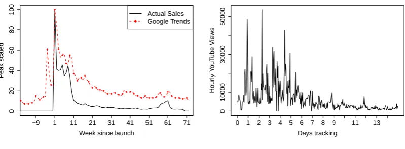
We provide two example time series for the two data types in Figure 1. The
example containing sales and search traffic is scaled for illustration purposes. Note
that for clarity the example of the YouTube video is without social shares. For the
“GoPro - Best of 2015” video clip we captured 3.6 million views and more than 25 thousand mentions on social networks (www.youtu.be/IyTv SR2uUo).
4.3. Experimental setup
Our aim is to assess the predictive usefulness of internet variables, across the life-cycles of the products, and follow the requirements laid out in Section 2.4. In
order to facilitate this, we employ a rolling window approach. The window has a
0 20 40 60 80 100
Week since launch
P
eak scaled
−9 1 11 21 31 41 51 61 71
Actual Sales Google Trends
(a) Battlefield 4 video game
0 10000 30000 50000 Days tracking Hour ly Y ouT ube Vie ws
0 1 2 3 4 5 6 7 8 9 11 13
[image:22.595.96.496.117.264.2](b) GoPro YouTube video
Figure 1: Sample time series
resulted in very poor forecasts and were excluded. The rolling window setup allows
us to consider the launch phase or the mature phase of the life-cycle of a product
separately.
At each forecast origin, we construct forecasts that rely on the additional
inter-net inputs and appropriate univariate benchmarks. For the additional variables to
be useful, they have to lead to more accurate out-of-sample forecasts. We assess
the performance at each forecast origin using the Average Relative Mean Absolute
Error (AvgRelMAE; Davydenko and Fildes, 2013):
AvgRelMAEi,h = n
v u u t n Y r=1 MAEi,r MAEb,r ,
MAE = 1
j
j
X
t=1
|yt+h−yˆt+h|,
wherenis the number of times series and j the number of forecast origins for each series. First, the Mean Absolute Error (MAE) across all origins, for a given time series and horizon is calculated for each forecasti. These are then divided by the MAE of the Na¨ıve forecast (MAEb,r) and summarised using a geometric mean to
produce the reported AvgRelMAE for each horizon.
com-parison between forecasts, where an improvement over the benchmark is given by
value lower than 1. Subtracting the AvgRelMAE from 1 provides the percentage
accuracy gain of a forecast over the benchmark.
Finally, to evaluate whether any differences are due to randomness or not, we
employ the non-parametric Friedman test and the post-hoc Nemenyi test (Koning et al., 2005; Demˇsar, 2006). We use the Friedman and Nemenyi tests as
imple-mented for R (R Core Team, 2016) in the TStools v.2.1.0 package (Kourentzes
[image:23.595.94.502.278.332.2]and Svetunkov, 2016).
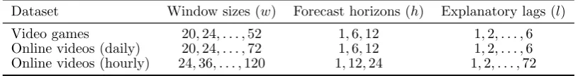
Table 3: Experimental settings for the different datasets
Dataset Window sizes (w) Forecast horizons (h) Explanatory lags (l) Video games 20,24, . . . ,52 1,6,12 1,2, . . . ,6 Online videos (daily) 20,24, . . . ,72 1,6,12 1,2, . . . ,6 Online videos (hourly) 24,36, . . . ,120 1,12,24 1,2, . . . ,72
4.4. Methods
We use the following regression model:
yt=α0+ m
X
i=1
αiyt-i+ k
X
j=1
βjxt-j +εt, (1)
whereytis the target variable andxtis the explanatory online information variable;
m and k represent the number of autoregressive terms and numbers of lags of the explanatory, respectively, and εt is a Gaussian zero-mean error.
As proposed by Hyndman and Khandakar (2008), we make our series stationary by using the KPSS and the OCSB tests to identify level and seasonal-differences,
respectively. This also eliminates any spurious connections betweenyt and xt. The challenge in (1) is the specification of m and k. Furthermore, one can consider sparse specification, as not all lags may be informative (Hastie et al.,
2015). In the aforementioned literature different approaches have been employed
to specify the relevant lags. Granger causality is one of them (e.g. Ruohonen and
Hyrynsalmi, 2017; Tirunillai and Tellis, 2012). Another popular modelling
example, as in Hyndman and Khandakar, 2008). However, note that in the
pres-ence of explanatory variables the number of potential models becomes prohibitive
very quickly. A stepwise approach can be used to manage the problem, however the
stepwise search strategy has been criticised for inadequate search of alternatives,
due to its greedy search nature (Hastie et al., 2015). The problem is exacerbated further by limited sample size.
Considering the case where all social network information is available, in the
extreme case, our model needs to estimate up to 297 parameters using only 24
observations. To solve this problem we rely on lasso regression that provides an
effective and efficient search of the model space and achieves sparsity, if needed,
even when the number of coefficients exceeds the available sample size. Lasso
works by penalising the model fit with the absolute of the sum of the coefficients,
scaled by a shrinkage factor. This forces the coefficient of uninformative variables
to zero. For details of lasso, as well as a discussion of alternative selection schemes
see Hastie et al. (2015). We fit the lasso regression using R and the package glmnet v.2.0-5 (Friedman et al., 2016) with its default settings.
Hereafter, we refer to these forecasts as ARX for the video games dataset
and ARX (FB) or ARX (All) if only shares in Facebook or more platforms are
considered for the video dataset.
We allow up to 6 autoregressive terms. For the hourly dataset we include
additionally up to 3 seasonal autoregressive terms. Furthermore, the model is
augmented by up to l lags of the explanatory variables (Table 3). To simulate a true forecasting situation we restrict the included lags to always be of order at
least equal to the forecast horizon or longer, as the in-between values would not be available. For example to forecast 3-steps ahead only lags of order 3 or more
are considered, as shorter lags would imply knowledge of the future values of the
explanatory variable.
To further complete our experiment we also discuss the case where we allow
contemporaneous explanatory variables in our model, producing now-casting
re-sults. Although this is of limited operational benefit, it allows us to relate our
experiment with the nowcasting literature that has used such variables.
We compare our ARX forecasts against various benchmarks from different
the same specification method to ARX. Second, we include an ARIMA model, the
orders which are identified using AIC corrected for sample size (AICc), based on
the model selection procedure by Hyndman and Khandakar (2008). Furthermore,
we use exponential smoothing, the form of which is automatically selected by
us-ing AICc (Hyndman et al., 2008). Finally, we include a Random Walk (Na¨ıve) forecast. In cases where the hourly online video time series is seasonal, we further
add a seasonal Na¨ıve as a benchmark. The benchmarks are implemented using
the forecast v.7.2 package for R (Hyndman, 2016).
4.5. Results
4.5.1. Overall results
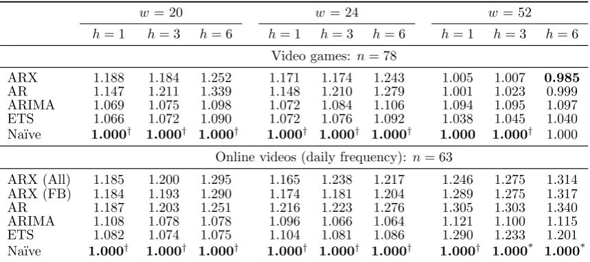
Table 4 presents the results for window sizes w = {20,24,52} and for fore-casting horizons h={1,3,6} weeks, across the complete life-cycle for both video game and online video dataset. Results for other tested windows between 24 and
52 weeks are very similar and therefore omitted. The striking result is that the
Na¨ıve is consistently the best or at least as good (with no significant statistical
[image:25.595.90.520.430.621.2]differences) as its competitors, followed closely by ETS and ARIMA.
Table 4: Overall forecasting performance across all origins
w= 20 w = 24 w= 52
h= 1 h= 3 h= 6 h= 1 h= 3 h= 6 h= 1 h= 3 h= 6
Video games: n= 78
ARX 1.188 1.184 1.252 1.171 1.174 1.243 1.005 1.007 0.985
AR 1.147 1.211 1.339 1.148 1.210 1.279 1.001 1.023 0.999 ARIMA 1.069 1.075 1.098 1.072 1.084 1.106 1.094 1.095 1.097 ETS 1.066 1.072 1.090 1.072 1.076 1.092 1.038 1.045 1.040 Na¨ıve 1.000† 1.000† 1.000† 1.000† 1.000† 1.000† 1.000 1.000† 1.000
Online videos (daily frequency): n= 63
ARX (All) 1.185 1.200 1.295 1.165 1.238 1.217 1.246 1.275 1.314 ARX (FB) 1.184 1.193 1.290 1.174 1.181 1.204 1.289 1.275 1.317 AR 1.187 1.203 1.251 1.216 1.223 1.276 1.305 1.303 1.340 ARIMA 1.108 1.078 1.078 1.096 1.066 1.064 1.121 1.100 1.115 ETS 1.082 1.074 1.075 1.104 1.081 1.086 1.290 1.233 1.201 Na¨ıve 1.000† 1.000† 1.000† 1.000† 1.000† 1.000† 1.000† 1.000* 1.000*
†Different at 95%-significance to ARX and all other benchmark models.
*Different at 95%-significance to ARX model
In most cases, the worst performing model is the simple AR that is
online video dataset. We find, no evidence that this difference is significant. On
the one hand, this supports findings from the literature that search traffic can
improve forecasts, but on the other hand, it also verifies our criticism of weak
experimental design. When benchmarked against more appropriate univariate
al-ternatives, here all ETS, ARIMA and Na¨ıve, we cannot support that conclusion. Closer examination of the individual time series reveals that in the presence of
ad-equate benchmarks there is no case where ARX ranks first across all benchmarks,
but it is easy to identify a single benchmark that would typically be worse than
ARX. The need for thorough benchmarking has been fundamental in
forecast-ing research (Armstrong and Collopy, 1992) and contrastforecast-ing our results with the
mostly positive impression from the literature helps to highlight how important
that is.
4.5.2. High frequency and nowcasting
Table 5 provides the results for the hourly time series. Although the forecast
horizons are now too short to support many operational decisions, looking at
higher frequency data allows us to explore whether intra-day lags may be more
informative. In this scenario, although the Na¨ıve is no longer best, overall we do
not observe benefits from including the additional variables. In fact, AR is in all
cases more accurate than either ARX (All) or ARX (FB). For longer window sizes
[image:26.595.88.543.516.630.2](w= 120) ARX (FB) outperforms the Na¨ıve, but is in turn outperformed by other univariate benchmarks.
Table 5: Overall forecasting results online videos (hourly) n= 63
w= 24 w= 72 w= 120
h= 1 h= 12 h= 24 h= 1 h= 12 h= 24 h= 1 h= 12 h= 24
ARX (All) 1.083 1.114 1.231 1.080 1.066 1.114 1.021 1.011 1.029 ARX (FB) 1.057 1.113 1.222 1.018 1.018 1.052 0.981 0.996 1.018 AR 1.002 1.058 1.198 0.951 0.953 0.972 0.941 0.935 0.939 ETS 0.953* 0.970* 0.993 0.943 0.901* 0.913 0.942 0.853* 0.856*
ARIMA 0.984 1.000 1.032 0.942 0.902 0.894* 0.935 0.881 0.871 Na¨ıve 1.000 1.000 1.000 1.000 1.000 1.000 1.000 1.000 1.000 sNa¨ıve 1.407 1.041 0.975* 1.368 1.004 0.953 1.363 0.992 0.945
*Different at 95%-significance to ARX model.
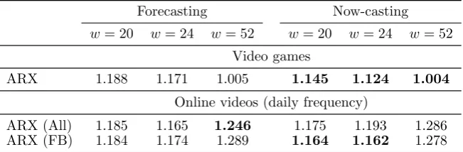
Table 6 presents the now-casting results. For convenience, we provide the
two is that the latter permits contemporaneous inputs of the variables. The results
suggest that there are improvements, yet still the Na¨ıve is more accurate for both
[image:27.595.136.462.185.292.2]datasets.
Table 6: Now-casting versus one step-ahead forecasting performance Forecasting Now-casting
w= 20 w= 24 w= 52 w= 20 w= 24 w= 52
Video games
ARX 1.188 1.171 1.005 1.145 1.124 1.004
Online videos (daily frequency)
ARX (All) 1.185 1.165 1.246 1.175 1.193 1.286 ARX (FB) 1.184 1.174 1.289 1.164 1.162 1.278
4.5.3. Performance across life-cycle stages
Since the search traffic seems not to add much value over the entire life-cycle, we
investigate different life-cycle stages. Table 7 presents the results for the scenario
of three-week-ahead forecasts with a window size of 20, for different weeks since
launch. Recalling the typical nature of the demand pattern shown in Figure 1a, one
would expect that search traffic information would be particularly useful towards
the beginning of the life-cycle, where there are lots of spikes. However, as we can see from the results, ARX performs poorly for the first few origins and only towards
the end of life it starts to outperform the simpler AR model. In this sense, the
forecasting performance of the search traffic model is much worse during the first
year of sales than any univariate model. We found this behaviour to be consistent
with other window sizes and forecasting horizons.
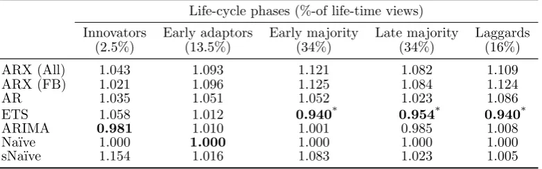
Table 8 provides the forecasting results for the online videos across life-cycle.
We classify the life-cycle phases according to Rogers (2003), with the splits
ac-counting for the percentage of total views. The results show that social network
information is not able to deliver additional forecasting performance in any of the life-cycle phases and the forecasting performance is quite consistent during the
Table 7: Forecasting performance for video games over life-cycle Weeks after launch
28-35 36-43 44-51 52-EOL ARX 1.665 1.308 1.200 1.110 AR 1.560 1.292 1.184 1.161 ETS 1.046 1.119 1.046 1.071 ARIMA 1.244 1.190 1.081 1.049 Na¨ıve 1.000* 1.000† 1.000† 1.000†
w= 20,h= 3
† Different at 95%-significance to ARX and all
other benchmark models.
*Different at 95%-significance to ARX model.
Table 8: Forecasting performance for online videos over life-cycle Life-cycle phases (%-of life-time views)
Innovators Early adaptors Early majority Late majority Laggards (2.5%) (13.5%) (34%) (34%) (16%) ARX (All) 1.043 1.093 1.121 1.082 1.109 ARX (FB) 1.021 1.096 1.125 1.084 1.124 AR 1.035 1.051 1.052 1.023 1.086 ETS 1.058 1.012 0.940* 0.954* 0.940*
ARIMA 0.981 1.010 1.001 0.985 1.008 Na¨ıve 1.000 1.000 1.000 1.000 1.000 sNa¨ıve 1.154 1.016 1.083 1.023 1.005
w= 24,h= 12
*Different at 95%-significance to ARX model.
5. Discussion
5.1. Reasons for poor performance
The reader may ask why did the models with the explanatory variables from
online platforms perform so poorly compared to the benchmarks? Or why did the
Na¨ıve perform that well? Both datasets contain noisy time series with demand
spikes, due to renewed interest by the consumers/viewers. Such time series are
notoriously difficult to predict without causal information, which can explain the
competitiveness of the Na¨ıve forecast against the other univariate forecasts. This
paper set out to evaluate the usefulness of online platform variables for this
pur-pose. We found that in many cases the ARX forecasts outperformed some of the benchmarks, but in no cases, all of them, and overall the impression was that the
[image:28.595.106.497.292.414.2]Although our empirical evaluation has its limitations, and we do not claim that
the results generally hold for other applications and datasets, it should encourage
researchers and practitioners to think critically about the predictive capabilities
of such data.
As discussed in Section 2, a large number of publications were not strictly in a predictive setup, or when such was used, the forecast horizons were too short
to support operational decision making. Requiring forecasts for longer horizons
implies an expectation that any causality between internet search traffic or social
network shares and sales will hold. However, it is not uncommon that internet
searches and buying decisions are made instantly or with a very short lag. Such
impulsive buying decisions do not allow the manager to take any reactive
opera-tional decisions. Our experiments support this interpretation and also agree with
the findings by Ruohonen and Hyrynsalmi (2017) who raise similar concerns. It is
unfortunate that the surveyed literature has mostly neglected this; reporting
fore-casting results that do not match realistic applications does not add new insights into the usefulness of such information.
As we have highlighted in Section 2.4, an unhelpful characteristic of many of the
published papers has been their weak experimental design, in particular concerning
their choice of benchmarks. In our two case studies, we found many cases were the
ARX model outperformed single benchmarks, typically its univariate equivalent,
but when tested against a set of well known and reliable univariate models it was
never the best performing. We have stressed the need for thorough evaluation
(Armstrong, 2006; Armstrong and Collopy, 1992). However many publications, in
this relatively new modelling research, come from various disciplines that do not strongly adhere to these principles. Therefore, it is important to retain a critical
view of the usefulness of such information against well established and tested
forecasting models. This is particularly relevant for practitioners, who would need
to invest in developing new systems.
5.2. Challenges in practice
There are many potential pitfalls when collecting data from internet sources
which we discussed in Section 3. For instance, we underestimated the effort needed
many arbitrary spikes and changes in volume. We assume that these numbers vary
because of potential click bait validation and synchronisation between servers.
User generated content has been praised for its availability at high frequency,
i.e. hourly or even minutes (Tirunillai and Tellis, 2012). However, at a high
sam-pling frequency, the collected values may become unreliable, which may also ex-plain to some extent the weak forecasting in our results. While the fast data-stream
allows for very granular sampling rate, increased volatility, multiple-seasonalities
and intermittency are introduced.
One further complication in practice might be how timely the data becomes
available. Most studies, including the one at hand, collect the data ex-post which
makes it relatively easy to find matchings keywords. However, given a relatively
new product, such signals might not be easy to identify, as search volume or reviews
need to build up first. There is a lack of research as to when such signals appear
strong enough and when they decline towards the end of the product life-cycle.
As discussed in Section 3.3, a further complication can be the selection of keywords. In our case, we used the video game title, which turned out to be highly
correlated to sales. In practice, not all products or services will have such a distinct
search keyword, and the signal can become distorted by unrelated search events to
the product in question. Another issue is that the desired keyword may have too
little search volume (Barreira et al., 2013). This limitation becomes more severe
when looking at a disaggregate level. Cui et al. (2017) and Seebach et al. (2011)
both suggest using hierarchical disaggregation methods for generating SKU level
forecasts. However, we are unaware of any study that evaluates the forecasting
performance of categorical and geographical disaggregation methods with internet platform data.
6. Conclusions
In this paper, we investigated whether search traffic and social network shares
are helpful in improving demand forecasting. We first looked at the existing lit-erature and identified limitations regarding their experimental design, both from
a statistical and practical point of view. Although the majority of publications
argued favourably as to the value of such data, our recommendation for researchers
From a forecasting point of view, we did not find substantial differences
regard-ing predictive power in different phases of the life-cycle. However, it is beyond the
scope of this study to explore the usefulness of this information prior to launch.
There is active research in this area with promising findings (e.g. Kim et al., 2015;
Xiong and Bharadwaj, 2014; Kulkarni et al., 2012). It may still be very useful in different forecast settings, such as nowcasting or by providing insights into
con-sumer behaviour. However, we underline the need for adequate benchmarking
and thorough forecast evaluation. All benchmarks used in this study are well
re-searched and understood forecasting models, which nowadays are trivial to deploy
and automate in a practical setting. At least, these should be outperformed before
the inclusion of additional explanatory variables would be warranted. Researchers
and practitioners should also be aware of the data complexity, potential biases and
dependency from the platform providers.
Naturally, our evaluation has limitations, but it supports aspects of our critical
stance towards the literature. One could argue that our comparison is unfair since ARIMA or ETS could also be augmented with additional variables. Although this
is a limitation of our design, specifying ARIMA or ETS with automated
explana-tory variable selection is challenging and neither approach lend to readily select
variables with a lasso. We also looked exclusively at linear models and preferred
modelling approaches that could be automated and scaled up, reflecting the needs
of the practice. Although we did not find any evidence of non-linearity by
explor-ing the datasets in our case studies, this will not be true for every application. For
example, Cui et al. (2017) postulate that non-linear models are the most effective
to include social media information. Our work leaves space for experimenting with more exotic linear or non-linear models.
A. Supporting tables for the literature review
Supplementary tables to this article are available online.
References
viewership. In: Proceedings of the 7th ACM International Conference on Web Search and Data Mining. WSDM ’14. ACM, New York, pp. 593–602.
Aral, S., 2014. The problem with online ratings. MIT Sloan Management Review 55 (2), 47–52.
Araz, O. M., Bentley, D., Muelleman, R. L., 2014. Using google flu trends data in forecasting influenza-likeillness related ed visits in omaha, nebraska. The Amer-ican Journal of Emergency Medicine 32 (9), 1016 – 1023.
Armstrong, J., Collopy, F., 1992. Error measures for generalizing about forecasting methods: Empirical comparisons. International Journal of Forecasting 8 (1), 69 – 80.
Armstrong, J. S., 2006. Findings from evidence-based forecasting: Methods for reducing forecast error. International Journal of Forecasting 22 (3), 583 – 598.
Babic Rosario, A., Sotgiu, F., De Valck, K., Bijmolt, T. H., 2016. The effect of electronic word of mouth on sales: A meta-analytic review of platform, product, and metric factors. Journal of Marketing Research 53 (3), 297–318.
Baccianella, S., Esuli, A., Sebastiani, F., 2010. Sentiwordnet 3.0: An enhanced lexical resource for sentiment analysis and opinion mining. In: LREC. Vol. 10. pp. 2200–2204.
Bangwayo-Skeete, P. F., Skeete, R. W., 2015. Can Google data improve the fore-casting performance of tourist arrivals? mixed-data sampling approach. Tourism Management 46, 454 – 464.
Barash, V., Ducheneaut, N., Isaacs, E., Bellotti, V., 2010. Faceplant: Impression (mis) management in facebook status updates. In: ICWSM. pp. 207–210.
Barreira, N., Godinho, P., Melo, P., Nov 2013. Nowcasting unemployment rate and new car sales in south-western europe with google trends. NETNOMICS: Economic Research and Electronic Networking 14 (3), 129–165.
Bijl, L., Kringhaug, G., Moln´ar, P., Sandvik, E., 2016. Google searches and stock returns. International Review of Financial Analysis 45, 150 – 156.
Bollen, J., Mao, H., Zeng, X., 2011. Twitter mood predicts the stock market. Journal of Computational Science 2 (1), 1 – 8.