Coevolution of Technical Trading Rules for High Frequency Trading

Coevolution of Technical Trading Rules for High

Frequency Trading

Kamal Adamu, Steve Phelps

Abstract—.Traders make trade decisions specifying entry,exit, andstop lossprices. Technicians often de-cide on entry, exit, and stop loss prices based on a predefined set of technical rules. In this paper, we employ a method based on grammatical evolution to coevolve technical rules for entry, exit, and stop loss for trading a London Stock Exchange (LSE) based stock in high frequency. We consider the case of two class of investors with risk averse, and loss prefer-ences and build a partial trading frontier given the preferences considered. The performance of the rules evolved is compared to a publicly available trading system called the turtle trading system (TTS) and the best rules produced by our method outperforms TTS.

Keywords: Coevolution, Grammatical Evolution, Trad-ing Systems, Turtle TradTrad-ing System, High Frequency Trading.

1

Introduction

Traders make trade decisions specifyingentry, exit, and stop lossprices. Theentryrule dictates when to enter the market, the exit rule dictates when to exit the market, and thestop lossrule dictates when toexit a losing trade. There exists an interdependency between these prices [3, 6]. A trader that consistently fails toexit a loosing trade when they have incurred a tolerable amount of loss will almost certainly be wiped out after a couple of loosing trades. Moreover, a trader that takes profit too early or too late before making a required amount of profit will have very little to cover their costs and loss or loose part of the profit she has made [3, 6]. Technicians decide on entry,exit, andstop lossprices based on technical trading rules [3]. However, as the amount of candidate indicators increases, the search space of trading rules grows larger and more complex.

In a previous paper we employ a method based on gram-matical evolution to coevolve technical trading rules for entry, exit, and stop lossfor low frequency trading. The performance of the rules in [4] is assessed using the Sharpe ratio [4] and the objective is to find a collaborating set of entry,exit, andstop loss rules that maximise the Sharpe

∗_{Center for Computational Finance and Economic Agents} Uni-versity of Essex, CO4 3SQ, UK. Email: [email protected], [email protected]

ratio. In [9] they employ a four tree genetic program-ming approach in developing trading rules for entering and exiting a long or short GBP/EUR trade. They as-sess the performance of the rules evolved using a power utility function under three major assumptions about the preference of agents namely, loss aversion, risk aversion, and risk neutrality. The performance of the rules evolved in [9] is evaluated as the average performance under the three preferences. In this paper, we employ the method we used in [4] to coevolveentry, exit, andstop loss rules for trading Amvesco (Amvesco is listed on the London Stock Exchange) in high frequency. The performance of the rules evolved is compared to a publicly available trad-ing system called the turtle tradtrad-ing system (TTS) [5, 6]. In addition, we compare the performance of our coevo-lutionary approach, which we will refer to henceforth as coevolutionary grammatical evolution (CGE), to a set of randomly distributed strategies. Similar to [9], we em-ploy a power utility function as our fitness function how-ever, we assess the performance of the rules evolved under three independent scenarios, risk aversion, and loss aver-sion and we build a partial trading frontier for these pref-erences (assuming a power utility, of course). Moreover, similar to [4, 9], we consider the case of a unit investor trading only one unit at any instant. The rest of the pa-per is organised as follows. Section 2 gives an overview of the TTS, coevolution, and Grammatical Evolution (GE). We present our data in Section 4, and a description of our framework is given in Section 3. We disccuss our re-sults in Section 5, and the paper ends with a conclusion in Section 6

2

Background

2.1

Turtle Trading System

Theentry, andexitrules, for the turtle trading system are specified in Algorithm 1, and Algorithm 2 respectively.

Ht, t ∈ {1,2,3,4...T} is the current highest price, and

Algorithm 1Entry rules for TTS if H_t> H_t−55 orH_t> H_t−20 then

GO LONG

else if L_t< L_t−55or L_t< L_t−20 then GO SHORT

Lt, t ∈ {1,2,3,4...T} is the current lowest price. The

entry, andexit rules of TTS are breakout rules. In other words, it is expected that if a global high (low) is made within a certain window (in this case a window of 55 bars or 20 bars) then there is a likelihood that prices will start to move in the direction of the breakout.

Algorithm 2Exit rules for TTS if L_t< H_t−20or L_t< L_t−10 then

Exit long position

else if H_t> L_t−20 orH_t> H_t−10 then Exit short position

end if

The TTS places the initial stop loss atentry using the following equation:

Stopt=

Stopt−1−2N if Long

Stopt−1+ 2N if short

(1)

whereN is the average true range and it is calculated as follows:

N = 19N_t−1TR_t/20 (2)

TR_t, t∈ {1,2,3,4...T} is thetrue range and its calcu-lated as follows:

TR_t= max(H_t−Lt, H_t−C_t−1, C_t−1−Lt) (3)

Ct, t∈ {1,2,3,4...T}is the price at the end of the time

intervalt, t∈ {1,2,3...T}.

2.2

Grammatical Evolution

In GE, initially a population of random integer strings is initialized. The integer strings are a numeric representa-tion of the solurepresenta-tions [1]. Solurepresenta-tions are mapped from in-teger strings to a human readable (executable) solutions using a set of production rules (grammar) [1].

The fitness of the mapped solutions is assessed and par-ents are selected for producing offspring solutions based on a roulette wheel principle [2]. Offspring solutions are mutated based on prespecified probabibity of mutation. Solutions with high fitness survive and pass down their genetic material to their offspring, and solutions with low fitness are replaced using tournament by solutions that surpass them in fitness. The process is repeated over sev-eral generations until a halting criterion is met.

2.3

Coevolution

Coevolution in the literature usually refers to a situa-tion where a trait in one species evolves in response to a change in the trait in another species [10]. In other words, it is a situation where one species exerts evolu-tionary pressure on the other causing it to evolve and

vise versa [10]. Coevolution in nature can either be co-operative, or competitive. Coevolutionary computation borrows from the idea of coevolution in nature. In co-evolutionary computing a problem is decomposed into subcomponents and the subcomponents are evolved si-multaneously. This way, interdependencies between the different subcomponents is taken into account [10]. For instance, in this paper the trading problem is divided into different but interdependent subcomponents.

3

Framework

In our framework, we coevolve entry rules for long po-sitions, exit rules for long positions, stop loss rules for long positions,entry rules for short positions,exit rules for short positions, and stop loss rules for short posi-tions. Each set of rule is a species on its own. We denote the species of entry rules for long positions as

Ei

L, i∈ {1,2,3...P}, the species ofexit rules for long

po-sitions asC_Li, i∈ {1,2,3...P}, and the stop loss rule for long positions asS_Li, i∈ {1,2,3...P}. E_S is the notation forentry rules for short positions, CS is the notation for exit rules for short positions, andSi_S, i ∈ {1,2,3...P} is the notation for entry rules for short positions. Sexual reproduction is inter-species and solutions are rewarded based on how well they contribute to the overall prob-lem. Collaborators are chosen at random from other species. For instance, when assessing a solution from the set E_Li, i ∈ {1,2,3...P}, collaborators are chosen at random from C_Li, i ∈ {1,2,3...P}, Si_L, i ∈ {1,2,3...P},

Ei

S, i ∈ {1,2,3...P}, CSi, i ∈ {1,2,3...P}, and SSi, i ∈

{1,2,3...P}. Each species asserts evolutionary pressure on the other. Solutions that contribute to solving the problem attain high fitness and survive to pass down their genetic material to their offspring. On the other hand, so-lutions that do not contribute are awarded low fitness and are eventually replaced by solutions with higher fitness. Algorithm 3 illustrates the algorithm for our coevolution-ary framework.

3.1

Utility Function

The framework for assessing the fitness of the rules pro-duced using CGE is as follows:

In this paper, we employ a power utility function as our fitness function [9]. The power utility function is defined by the following equation [9]:

U(W_i) = Wi

1−γ

1−γ − 1

1−γ, γ >1 (4)

Wi=

W0(1 +vi) vi>0

w0(1 +vi)λ vi<0, λ >1 (5)

Algorithm 3Framework for Coevolutionary Grammat-ical Evolution (CGE)

foreach populationdo

Initialise random population of integer strings Map integer strings

Evaluate fitness of population Check for best solution (elitist) end for

whilehalting criterion is not metdo foreach populationdo

Generate offspring solutions Map offspring solutions

Evaluate fitness of offspring solutions Select new population of solutions end for

Check for new elitist

Evaluate fitness of ecosystem end while

Algorithm 4Framework for fitness assesment if Entry rule for long position is metthen

Go Long

else if Entry rule for short position is metthen Go short

end if

if Long and (Exit rule for long position is met)then Exit long position

calculate utility of wealth

else if Stop rule for long positionthen Exit long position

calculate utility of wealth end if

if Short and (Exitrule for short position is met)then Exit short position

calculate utility of wealth

else if stop rule for short position is metthen Exit short position

calculate utility of wealth end if

Ii=

+1 Long position

−1 Short position (7)

vi is the return for trade interval i, i ∈ {1,2, ....N}, Wi

is a modified level of wealth for the given trade interval

i, i ∈ {1,2, ....N}, and I_i, i ∈ {1,2,3...N} is the trade indicator for a given trade interval. For this study we consider the case of a unit investor and set the initial level of wealthW₀= 1. λ, andγ define the risk, and loss preference of the agents respectively. The fitness,f, of a trading strategy is then taken to be the expected utility, which is calculated as follows:

f =E(Uˆ(W)) = 1

N

N

i

U(W) (8)

The following assumptions are implicit in the fitness eval-uation:

1. Only one position can be traded at any instant.

2. Only one unit can be traded at any instant.

3. The is no market friction (zero transaction cost, zero slippage, zero market impact). Arguably, since only one unit is traded at any instant, the effect of market impact can be be considered to be negligible.

Our objective is to find rules forentry,exit, andstop loss that maxisimise the expected utility,E(Uˆ(W)).

3.2

Parameter Settings

In this paper, we set the population size ofEi_L, E_Si, C_Li,

Ci

S,SiL,SSi to 50 (i.e N=50). Collaborators are chosen at

random for cooperation and this is done every generation (the epoch length for cooperation isepoch=1). The max-imum number of generations,G_max, is set to 200 and if afterG_max/2 there is no improvement in the mean fitness ofE_Li, the search is terminated and a new search is ini-tialised. We run 10 searches in this fashion. For one set of 10 searches we consider the case of a loss averse agent withγ=35 and λ=1.15. For a second set of 10 searches we consider the case of risk averse agents withγ=35, and

λ=1.

The grammar used in mappingEi_L, E_Si, C_Li, andC_Si is shown in Table 1 and the grammar used in mappingSi_L,

Si

S is shown in Table 2. In our notation, O(t-n:t-1)

rep-resents a set of open prices, C(t-n:t-1) reprep-resents a set of closing prices, H(t-n,t-1) represents a set of highest prices, and L(t-n:t-1) represents a set of lowest prices be-tween t-n and t-1. O(t-n) represents the open price at t-n, C(t-n) represents the closing price at t-n, H(t-n) rep-resents the highest price at t-n, and L(t-n) reprep-resents the lowest price at t-n. Where n ∈ {10,11,12...99} and

Table 1: Grammar for mappingEi_L,E_Si,C_Li, andC_Si. φ is the set of non terminals,r are the rules for mapping the non-terminalφ, and n is the number of rules for mapping the non-terminalφ

φ r n

<expr>:: <binop>(<expr>, <expr>)

<rule> (2)

<rule>:: <var><op><var>

<var><op><fun>

<fun><op><fun> (3)

<binop>:: and, or, xor (3)

<var>:: H(t−<window>)

L(t−<window>)

O(t−<window>)

C(t−<window>)

<op>:: >, <,=,≤,≥, (4)

<window>:: <integer><integer> (1)

<integer>:: 1, 2, 3, 4, 5, 6, 7, 8, 9 (9)

<fun>:: sma(H(t-<window>:t-1)) ema(H(t-<window>:t-1)) max(H(t-<window>:t-1)) min(H(t-<window>:t-1)) sma(L(t-<window>:t-1)) ema(L(t-<window>:t-1)) max(L(t-<window>:t-1)) min(L(t-<window>:t-1)) sma(O(t-<window>:t-1)) ema(O(t-<window>:t-1)) max(O(t-<window>:t-1)) min(O(t-<window>:t-1)) sma(C(t-<window>:t-1)) ema(C(t-<window>:t-1)) max(C(t-<window>:t-1))

min(C(t-<window>:t-1)) (15)

Table 2: Grammar for mappingS_Li, andS_Si. φis the set of non terminals, r are the rules for mapping the non-terminalφ, and n is the number of rules for mapping the non-terminalφ

φ r n

<expr>:: <preop>(<expr>,<expr>)

<rule> (2)

<rule>:: <rule><op><rule>

<var><op><var>

<var><op><fun>

<fun><op><fun>

<fun>

<var> (6)

<preop>:: min, max (2)

<var>:: H(t-<window>) L(t-<window>) O(t-<window>)

C(t-<window>) (4)

<fun>:: sma(H(t-<window>:t-1)) ema(H(t-<window>:t-1)) max(H(t-<window>:t-1)) min(H(t-<window>:t-1)) sma(L(t-<window>:t-1)) ema(L(t-<window>:t-1)) max(L(t-<window>:t-1)) min(L(t-<window>:t-1)) sma(O(t-<window>:t-1)) ema(O(t-<window>:t-1)) max(O(t-<window>:t-1)) min(O(t-<window>:t-1)) sma(C(t-<window>:t-1)) ema(C(t-<window>:t-1)) max(C(t-<window>:t-1)) min(C(t-<window>:t-1))(15)

<window>:: <integer><integer> (1)

4

Data

In this paper, we compress historical high frequency tic-data into a sequence of high, low, open, and close proxy prices for five minutely trading intervals [7]. The data we use is Amvesco tic-data for the period between 1 March 2007 to 1 April 2007. The descriptive statistics of the data is shown in Table 4

Table 3: Descriptive statistics of data Mean Standard deviation Skewness Kurtosis

-0.0193 1.6072 -1.4265 24.6282

Table 4:

The data was divided into four blocks for K-fold cross validation [8].

5

Results & Discussion

Table 5 shows the descriptive statistics for the set of loss averse agents (λ=1.15,γ=35) produced using CGE, the set of risk averse agents (λ=1, γ=35) produced us-ing CGE, and random strategies (MC) with loss averse (λ=1.15,γ=35), and risk averse (λ=1,γ=35) preferences. Also included in Table 5 is the expected utility obtained by the TTS for a risk averse (λ=1,γ=35), and loss averse (λ=1.15,γ=35) preference.

The results in Table 6 are results for a sign test for the null hypothesis that the median of the set of loss averse strategies produced using CGE is different from the ex-pected utility of the TTS with the same preference, and for the null hypothesis that the median of the set of risk averse strategies produced using CGE is different from the expected utility of the TTS with the same prefer-ence. The results in Table 6 indicates a failure to reject the hypothesis at 95% confidence interval. This means given the preferences considered we have not produced sets of strategies with medians that are statistically dif-ferent from the expected utility of TTS. However, the best strategies produced using CGE outperform TTS for both scenarious considered.

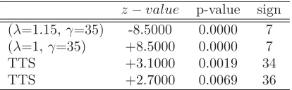
The results in Table 7 is for the null hypothesis that the median of the set of loss averse agents is different from the median of random strategies with the same preference. It also includes results for the null hypothesis that, the median of the set of risk averse agents is different from the median of a set of random strategies with the same preference, and the median of a set of random strategies is different from the expected utility of the TTS. The results in Table 7 show that we should reject the null at 95% confidence interval for all of the strategies.

Figure 1 shows the trading frontier from the two sets of strategies produced using CGE. μ_r, σ_r, α_r, and γ_r are

Table 5: Descriptive statistics of the distribution of utility for different strategies. μ is the mean,σ is the standard deviation, αis the skewness, andω is the kurtosis. MC is a set of random strategies

μ σ α ω

CGE(λ=1.15,γ=35) +0.0001 0.008 -1.49 5.31 CGE(λ=1,γ=35) -0.0055 0.007 -0.75 1.94 MC(λ=1.15,γ=35) -0.0018 0.008 -3.52 20.80 MC(λ=1,γ=35) -0.0003 0.003 -0.99 21.65 TTS (λ=1.15,γ=35) -0.001 0.0001 -1.10 2.29 TTS (λ=1,γ=35) -0.0003 0.0001 -1.05 2.24

Table 6: Sign test for the null hypothesis that the medians of the sets strategies produced using CGE is the same as the expected utility of the TTS with the same preference.

z-value p-value sign (λ=1.15,γ=35) 1.5811 0.10940 2 (λ=1,γ=35) -0.9487 0.34380 2

the mean, standard deviation, skewness, and kurtosis of the strategies respectively. Figure 1 shows that quite a number of loss averse CGE strategies dominate their risk averse strategies in the μ_r and σ_r frontier, and produce considerably positively skewed returns compared to their loss averse counterparts.

6

Conclusions and Future Work

Technical traders make trade decisions specifying entry exit, and stop loss prices based on technical trading rules. In this paper, we have coevolved rules that tell a trader when toenter the market, and when to exit the market for long, and short positions respectively as well as rules that tell a trader when toexita loss making position (stop loss). Two set of rules were produced for two different preferences. The performance of the rules produced is compared with a publicly available trading system called the turtle trading system (TTS) and the best rule pro-duced by our method outperforms the TTS. Our rules were also compared to a set of random strategies and the strategies produced by our method are statistically better

Table 7: Sign test for the null hypothesis that the medians of random strategies is same as the median of strategies produced using CGE, and for the null hypothesis that the median of random strategies is the same as the expected utility of the TTS

z−value p-value sign (λ=1.15,γ=35) -8.5000 0.0000 7 (λ=1,γ=35) +8.5000 0.0000 7

TTS +3.1000 0.0019 34

Figure 1: Trading frontier of CGE strategies for different preferences. μ_r is the mean return, σ_r is the standard deviation of return, α_r is the skewness of return, γ_r is the kurtosis of return

than random strategies in trading the stock of Amvesco for both of the preferences considered (i.e loss aversion, and risk aversion). The TTS is also shown to be statis-tically better than a set of random strategies in trading the stock of Amvesco. Moreover, we have generated a partial trading frontier and most of the loss averse strate-gies dominate the risk averse stratestrate-gies in the mean, and standard deviation setting, and produced highly skewed positive returns.

In this paper, we make an assumption of frictionless markets. In future work we will include transaction cost. Moreover, we will allow for multiple positions to be traded.

References

[1] O’Neill, M., Ryan, C.,Grammatical Evolution: Evo-lutionary Automatic Programming in an Arbitrary Language , Kluwer Academic Publishers, 2003.

[2] Fogel, B.F., Evolutionary Computation: Toward a New Philosophy of Machine Intelligence, IEEE Press, 1995.

[3] Murphy, M.J., Technical Analysis of the Futures Markets, New York Instituce of Finance, Prentice Hall, 1986.

[4] Adamu, K., Phelps., S,, “A Coevolutionary Gram-matical Evolution Approach for Developing Tech-nical Trading Rules,” Asia Pacific Industrial Engi-neering and Management Sys. Conf., Kitakyushu, Japan, pp. 187.

[5] Anderson, J.A., “Taking A peek Inside the Turtle’s Shell,”School of Economics and finance, Queensland University of Technology., Australia.

[6] Faith, C., “The original turtle trading system,” www.turtletrader.com

[7] Ahmad, K., Ahmad, S., “Reuters Data Analysis, Brand Protection: Comparing the Provenance of two Time Series,” University of Surrey Department of Computing2003

[8] Kohavi, R. “A study of Cross-Validation and Boot-strap for Acurracy Estimation and Model Selection,” International joint Conference on artificial intelli-gence,1995

[9] Saks, P., Maringer, D., “Evolutionary Money Man-agement,” Lecture Notes in Computer Science, Springer, V5484/2009, pp. 162-171