Scene Classification Using Efficient Low-level Feature Selection 1

Scene Classification Using Efficient Low-level

Feature Selection

1

Chu-Hui Lee, Chi-Hung Hsu

Abstract—With the development of digital cameras, the digital photographs were flooded in our life. How to classify images efficiently in huge image database becomes an important research topic. In recent years, the related researches of the image classification are based on semantics. The scene image classification has received much attention especially because it contains plenty semantics. It is a difficult challenge to classify the scene images accurately. This paper tries to use particle swarm optimization (PSO) algorithm that has biological characteristic, and to train with the scene images of semantics. We can get a scene transformation matrix during the process. The scene transformation matrix can be used to classify scene images, which are close to human’s semantics. The experiment shows our proposed method has great correct classification rate.

Index Terms—Particle swarm optimization, semantic, image classification, scene.

I. INTRODUCTION

How to manage images efficiently becomes more challenging and important issue today. Scene classification is one of solutions to organize the image database. The aim of scene classification is to label automatically among a set of meaningful semantic categories.

In recent years, researchers have been focusing on solve the semantic gap [1] [6] [10] [16] in the content of the images to support good scene classification, which can automatically capture the characteristics of images to be closer to human cognition. Many technologies have been derived such as using ontology to define high-level semantic concept and support semantic search. Besides, in the process of image retrieval, relevant feedback mechanism is added so that users can continuously adjust the retrieval images closer to the semantic requirements [8]. Adjusting from feedback will keep evolving and building connections between low-level feature information and high-level semantics [17].

However, low-level features can be mapped to know scene content, such as indoor, outdoor or landscapes. Many scholars have been involved in scene classification studies by low-level features such as top-down, bottom-up or mixture of the both of image object segmentation and identification, combination of SVM, K-NN and GMM and estimation of a

certain classification with Bayes probability, etc [2][3][5][11]. Basically, these researches are divided into two categories. The first one is classification with whole visual appearance and classifies image contents by global visual features. For example, the system proposed by Torralba and Oliva [13]. The other one is to segment images into some meaningful blobs and use them as semantic elements to classify image content.

The performance of PSO in image feature selection is noble. In our paper, we use particle swarm optimization (PSO) to find the correlations between low-level features and high-level semantics and reduce semantic gap. The query results are more closer to users’ semantic requirements. Though continuous PSO learing evolution, the system can acquire multi-scenes transformation matrix for classification. The experiements will show our provided method has great correct classification rate for the scene classification.

The structure of this research is: in Section II, PSO development and scene image classification are discussed. Section III explains how this research acquires a flexible scene transformation matrix with POS and classifies images through the scene transformation matrix. Section IV gives the experiemnt results and section V shows conclusions of this research.

II. PREVIOUS WORK

Currently, there are two structures of our research for scene image classification. We specify these two structures in this section.

A. Particle swarm optimization algorithm

Particle Swarm Optimization algorithm (PSO) is proposed by Kennedy and Eberhart in 1995 [9]. The main concept is derived from group behavior theory. In group actions of organisms, messages among individuals make the entire group move towards more suitable directions. This algorithm is to seek the maximum benefits of groups in imitation of organisms’ behaviors. The initial PSO is in uniform distribution to generate particle groups randomly. Each particle, with its own best Pbest and group’s best in experiences, modifies the movement directions. After continuous modifications, it is expected they will move to the optimal solution. The formula of particle calculation is:

Gbest

(

id

)

(

id

id C rand Pbest X C rand Gbest X

)

id V

V = + ₁⋅ ₁⋅ − + ₂⋅ ₂⋅ −

d i d

i V

X

(1)

d i

X = + (2)

finitions fo

ace

city) for the particle i in imal solution.

The de

di ___________________________________________________________

1_{This work was supported by National Science Council under Grant NSC}

96-2221-E-324-043. r the variables are listed in the following:

1) i : the ith particle. Chu-Hui Lee Author is with the Chaoyang University of Technology,

Wufong Township Taichung County, 41349 Taiwan (R.O.C.). Phone: 886-4-23323000 ext 4388; fax: 886-4-23742337; e-mail: chlee@ cyut.edu.tw.

2) d: the dimension sp

3) Vid: position change (velo the

Chih-Hung Hsu is with the Chaoyang University of Technology, Wufong Township Taichung County, 41349 Taiwan (R.O.C.). E-mail: [email protected].

5) Gbest: group optimal solution.

6) : position change (velocity) for the particle in the ant.

e between 0 and 1.

hrou city

rist

s the de

[image:2.595.361.510.236.368.2]

rticle sw

Fig. 2. The base p rm Optim ion [15]

id

X i

dimension d. 7) C1,C2: learning const

8) rand1,rand2: random variabl

T gh formula (1), one can acquire the position velo i

V

prev

d of each particle on the next step. The addition of the ious positionXid of each particle and the new position velocityVid is the next position of the particle. Applying the characte ic of organism heading towards the destination in image classification can, based on users’ requirements, find the significant features for each meaningful scene.

Fig. 1 shows that each particle moves toward

[image:2.595.55.258.302.439.2]

exper parti

Fig. 1. Movement of particles [15

Fig. 2 illu s of pa

stination. Before moving, each particle refers to its own best Pbestand group’s best Gbest in experiences. These two iences enable the cles move towards the destinations to generate the value closer to the optimal solution.

] strates the optimal algorithm proces

arm. Before algorithm, several particles are generated randomly for algorithm. After optimal algorithm of particle group, the particles closest to the destination are the current best solution.

rocess of Particle Swa izat

B. Low-level image features

There are many useful features in the images. The color features are suit for most consumer photos and texture feature are for nature scene. We will give some brief introductions for these two features.

1. Color features

In general, color is one of the most widely used low-level features. A lot of space of colors can be used such as RGB, LAB, HSV and YCrCb. HSV is closest to human vision effect among the color features. HSV color space is shown in Fig. 3. The value of H refers to hue between 0 and 360, the value of S that represents the saturation is between 0 and 1 and the value of V means the brightness is between 0 and 1. The three elements make up the color space.

Target  Gbest

Pbest

X Y

Fig. 3. HSV color space model [14]

Among the color features technologies, the color histogram proposed by Swain and Ballard is the most popular [12]. The color space is quantified into several bins. Each pixel in the image is distributed into the corresponding bin according the color feature. Values for every bin are recorded to acquire the color histogram of the image. The reason of the popularity is that histogram simply considers the frequency of each color. It can also keep the invariant after rotation of image.

Yes No

Generated particles position

Evaluate fitness

Assessing Pbest and Gbest

Updating particle position

Algorithm termination conditions

2. Texture features

In image classification, texture features express the contents in an image often [16]. For example, fig.4 is the image of blue sky and the other is that of blue ocean. It is difficult to correctly classify the two images with color features, as the two are mainly in blue. However, texture feature distinguishes the differences between the two images better than color features. As a result, texture is a significant feature for high-level semantic images classification.

(1) Sufficient good fitness

[image:2.595.82.246.508.755.2]

(2) Reaching the maximum generations

[image:2.595.348.507.639.712.2]

conducts image texture features in consideration of changes of grey scale values of the entire image pixel dots, aiming at the different distance between four angles (0, 45, 90 and 135 degrees).

)) (

( )

(Y Max y_i y₁ y₂ y_{i 1} y_{i 1} y_n

Fitness = − + +L ₋ + ₊ +L+ (4)

The fitness value of particles is used to estimate whether this particle can replace current and Gbest values. If the fitness value exceeds current , it replaces the fitness value to be the optimal . The same, it also applies to . If the fitness value is smaller than current Pbest

andGbest, then we do not replace and .

Pbest Pbest Pbest Pbest Gbest Gbest III. SCENE IMAGE CLASSIFICATION

Scene images contain a lot of rich semantic information. Under the goal of getting closer to users’ semantics, classifying each image into the appropriate category is an important challenge.

Replacement of Pbest andGbest:

j

j fitness Pbest then Pbest X

X fitness

If ( )> ( ) = (5)

j

j fitnessGbest thenGbest X

X fitness

If ( )> ( ) = (6)

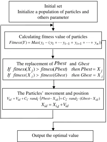
[image:3.595.304.533.237.540.2] [image:3.595.74.257.253.480.2]

This research extracts the low-level features of each image and has semantic learning through PSO. After a series of training, the system image can find a proper scene transformation matrix. After applying transformation matrix, one can then locate the best possible category of the images for classification. The entire process is as Fig. 5.

Fig. 5. Scene image classification process

The replacing process in formulation (5) considered one particle (one image) only. And the replacing process in formulation (6) considered the all particles (all images) in the algorithm.

A transformation matrix is denoted as , where n represents the number of scenes and m represents the number of image features. The low-level feature of an image is denoted as m n Scene× ) m

{

y₁,y₂,y₃

=

,v

n

y

Y ,_L,

, , , (v1 v2 v3

image

P= _K

}

. The scene classification vector is represented as . The goal of the PSO procedure is to find a proper

that helps to map low-level features to scenes. The mapping mechanism is achieved by the operation of product

of and

m n

Scene_×

m n

Scene_× (v₁,v₂,v₃,_K,v_m)

1

1 ×

×

×m× m = n

n P Y

Scene

m n

X _×

image

P= , that is

(3) Before entering PSO procedure, we need to set many parameters, such as movement speed of particles and generate the initial position of particles randomly.

During the PSO training process, the scene transformation is then made on each image. The feature vector

) , , , ,

(v₁ v₂ v₃ v_m image

P= _K and the classification, assumed that is , of image are known at preparing stage. Then we can acquire a meaningful n dimensions vector of scene

classificationY by

th

i

{

y1,y2,y3,L,yn

}

= Xn×m ×Pm×1=Yn×1.

Calculation of particle fitness’s value:

Fig. 6. The detail process of Particle Swarm Optimization Calculating the movement with current Pbest and

for each particle, all particles move towards . After a series of training, optimal solution is acquired.

Gbest Gbest

The calculation of particles’ movement:

(

id

)

(

id

id

id V C rand Pbest X C rand Gbest X

V = + 1⋅ 1⋅ − + 2⋅ 2⋅ −

)

(7)

The current position adds the movement of the particle is the new target position.

New target position of the particle: id

id d

i X V

X = + (8) After Particle Swarm Optimization algorithm, we acquired a flexible scene transformation matrix that can be used to calssify images. For classifying image

m n

Gbest _×

'

P , we calculate Gbest_n×m×P'=Y' and , in which

{

,y_n'

}

'

Y= y₁',y₂',_L

{

}

{ }

yj'

Maxy1',y2',L,yn' = classifies the image into

the j_th scene classification. Initial set

Initialize a population of particles and others parameter 

Extracting image low-level features

Calculating fitness value of particles )) (

( )

(Y Max y_i y₁ y_{i 1} y_{i 1} y_n

Fitness = − +_{L −} + ₊ +_L+

 

The replacement of

Pbest

and Gbest

Pbest _j

j fitness then X

X fitness

If ( )> (Pbest) =

j

j fitness Gbest thenGbest X

X fitness

If ( )> ( ) =

Acquiring scene transformation matrix by PSO

The Particles’ movement and position

(

)

_{2 2} ( )

1

1 id id

id

id V C rand Pbest X C rand Gbest X

V = + ⋅ ⋅ − + ⋅ ⋅ −

id d i

id X V

X = +  

Output the optimal value Calculation of transformation matrix

P

Scene_n×m×  

Scene classification

IV. EXPERIMENT

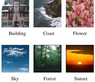
We implement the experiments in Microsoft Visio Basic 6.0. The computer is HP Desktop Series used AMD Athlon™ 64X2 Dual Core Processor 3800+ MHz and 1.99 GB RAM. The system is Microsoft Windows XP Professional. Most of the test images were downloaded from http://wang.ist.psu.edu/docs/relatedUUTT. We choice six different classifications that are building、coast、 flower、sky、forest and sunset. Those classifications contained 115、99、124、70、122 and 104 color images respectively and the amount of images is 634. All of them had dimensions of 100X100 pixels. The example images of each scene are given in Figs.7.

Building Coast Flower

[image:4.595.324.552.49.187.2]

Sky Forest Sunset Fig. 7. The example images of each scene

In the experiment, we extracted two low-level features that are color and texture for each images. In color feature, we use HSV color space and quantify into 40 bins which composed of 10 bins、 2 bins and 2 bins respectively. In texture feature, we used Gray-level Co-occurrence matrix to compute four features that are Entropy、Angular Second Moment、Contrast and Inverse Difference Moment. Then we quantify four features into 24 bins. Final, we use the 40 bins color feature and 24 bins texture feature composed 64 bins for low-level image features.

The performances of our proposed method are measured by formula (9). There are total twenty times in our experiments. The average performance of results is shown in table1and fig.8. The average of correct classification images amount is 540 and average of each scene correct classification rates is between 72.85% and 89.52%. As it is clearly stated, worse results were obtained by the sky scene classification and the correct classification rate is 72.85%. However, a 85.17% of overall correct classification rates is achieved by our experiment.

image Test image tion classifica Correct

R C

C. . = (9)

Table 1、The average performance of twenty times scene image classification

Average of results

Scenes Test image Correct C.C.R

Building 115 97 84.34%

Coast 99 87 87.88% Flower 124 112 89.52%

Sky 70 51 72.85%

Forest 122 102 83.60%

Sunset 104 91 87.50%

Total 634 540 85.17%

60 70 80 90 100

Building Coast Flower Sky Forest Sunset Scenes

C

o

rr

ect

cl

as

si

fi

ca

ti

o

n

r

at

e

（%

） C.C.R.

[image:4.595.68.262.202.370.2]

Average

Fig.8. The average performance of each scene image classification

In our experiment, we can find the difference between average performance rate and the best performance rate is 11.2%. The cause is initial particles of Particle Swarm Optimization algorithms are generated randomly and evolve into helpful particles by alternation of generations. This indicates that the experiment result would be influenced by initial particles. However, we can reduce the influence by evolving of longer generations. As the result is clearly stated, our experiment performed well.

V. CONCLUSION

In this paper, we used image’s low-level features and applied Particle Swarm Optimization algorithm to get a transformation matrix that can classify several scenes at once. The results of scene transformation matrix are close to human’s semantics as experiment shown. However, objects in the images represent important semantics in many scenes. We will take the object semantics into consideration for the further research.

REFERENCES

[1]Zaher Aghbari , Akifumi Makinouchi,’’ Semantic Approach to Image Database Classification and Retrieval,’’ NII Journal, No.7, 2005

[2]Anna Bosch, Robert Marti and Xavier Munoz, “Which is the best way to organize/classifiy images by content? ,” Image and Vision Computing, Vol 25, pp.778-791, 2007

[3]A. Casals, J. Batlle, J. Freixenet and J. Marti, “A review on strategies for recognizing natural objects in colour images of outdoor scenes,” Image and Vision Computing, Vol 18, pp.515-530, 2000 [4]I. Dinstein, K. Shanmugam and R.M. Haralick,

“Texture features for image classification,” IEEE Transactions on Systems, Man and Cybernetics, Vol.3, No. 6, pp. 610-621.

[5]J. Fan, Y. Gao, H. Luo and G. Xu, “Statistical modeling and conceptualization of natural images,” Pattern Recognition, Vol.38, pp.865-885, 2005 [6]Jianping Fan and Yuli Gao, “Semantic Image

Classification with Hierarchical Feature Subset Selection,” November 10-11, MIR, Singapore, 2005 [7]Image.vary.jpg.tar, www-db.Stanford.edu.

[image:4.595.59.280.657.781.2]

Proceeding of the ICIP, Vol.II, pp.511-514, 2003 [9]J. Kennedy and R. C. Eberhart, “Particle Swarm

Optimization,” Proceedings IEEE Int’l. Conf. on Neural Networks, IV, pp.1942-1948, 1995.

[10]J. Shen, J. Shepherd, A.H.H. Ngu,

“Semantic-sensitive classification for large image libraries,” International Multimedia Modelling Conference, Melbourne, Australia, pp.340-345, 2005

[11]A.E. Savakis, A. Singhal and J. Luo, “A Bayesian network-based framework for semantic image understanding,” Pattern Recognition, Vol.38, pp-919-934, 2005

[12]M. J. Swain and D. H. Ballard, “Color indexing,” International Journal of Computer Vision, Vol. 7, No. 1, pp. 11-32.

[13]A. B. Torralba and A. Oliva. “Semantic organization of Scenes using discriminant structural templates.” In ICCV, No. 2, 1999.

[14]J. Wales, HSV Color Space, Wikipedia encyclopedia, Mar 2002

[15]Xiangyang Wang, Jie Yang, Xiaolong Teng, Weijun Xia and Richard Jensen, “Feature Selection Based on Rough Sets and Particle Swarm Optimization,” Pattern Recognition Letter, pp.459-471, 2007

[16]Dengsheng Zhang, Guojun Lu, Wei-Ying Ma and Ying Liu, “A survey of content-based image retrieval with high-level semantics,” Pattern Recognition, Vol 40, pp.262-282, 2007