Robust Gram Embeddings
Taygun Kekec¸ and D.M.J. Tax
Pattern Recognition and Bioinformatics Laboratory Delft University of Technology
Delft, 2628CD, The Netherlands
[email protected],[email protected]
Abstract
Word embedding models learn vectorial word representations that can be used in a variety of NLP applications. When training data is scarce, these models risk losing their gener-alization abilities due to the complexity of the models and the overfitting to finite data. We propose a regularized embedding formu-lation, calledRobust Gram (RG), which pe-nalizes overfitting by suppressing the dispar-ity between target and context embeddings. Our experimental analysis shows that the RG model trained on small datasets generalizes better compared to alternatives, is more robust to variations in the training set, and correlates well to human similarities in a set of word sim-ilarity tasks.
1 Introduction
Word embeddings represent each word as a unique vector in a linear vector space, encoding particular semantic and syntactic structure of the natural lan-guage (Arora et al., 2016). In various lingual tasks, these sequence prediction models shown superior re-sults over the traditional count-based models (Ba-roni et al., 2014). Tasks such as sentiment analysis (Maas et al., 2011) and sarcasm detection (Ghosh et al., 2015) enjoys the merits of these features.
These word embeddings optimize features and predictors simultaneously, which can be interpreted as a factorization of the word cooccurence matrix C. In most realistic scenarios these models have to be learned from a small training set. Furthermore, word distributions are often skewed, and optimiz-ing the reconstruction of Cˆ puts too much
empha-sis on the high frequency pairs (Levy and Goldberg, 2014). On the other hand, by having an unlucky and scarce data sample, the estimatedCˆrapidly deviates
from the underlying true cooccurence, in particu-lar for low-frequency pairs (Lemaire and Denhire, 2008). Finally, noise (caused by stemming, removal of high frequency pairs, typographical errors, etc.) can increase the estimation error heavily (Arora et al., 2015).
It is challenging to derive a computationally tractable algorithm that solves all these problems. Spectral factorization approaches usually employ Laplace smoothing or a type of SVD weighting to alleviate the effect of the noise (Turney and Pantel, 2010). Alternatively, iteratively optimized embed-dings such as Skip Gram (SG) model (Mikolov et al., 2013b) developed various mechanisms such as undersampling of highly frequent hub words apriori, and throwing rare words out of the training.
Here we propose a fast, effective and general-izable embedding approach, called Robust Gram, that penalizes complexity arising from the factorized embedding spaces. This design alleviates the need from tuning the aforementioned pseudo-priors and the preprocessing procedures. Experimental results show that our regularized model 1) generalizes bet-ter given a small set of samples while other methods yield insufficient generalization 2) is more robust to arbitrary perturbations in the sample set and alterna-tions in the preprocessing specificaalterna-tions 3) achieves much better performance on word similarity task, especially when similarity pairs contains unique and hardly observed words in the vocabulary.
2 Robust Gram Embeddings
Let|y|=V the vocabulary size and N be the total number of training samples. Denotex, yto beV×1
discrete word indicators for the context and target: corresponding to the context and word indicators c, w in word embedding literature. Define Ψd×V
and Φd×V as word and context embedding
matri-ces. The projection on the matrix column space,Φx,
gives us the embedding~x∈Rd. We useΦxandΦ x
interchangeably. Using a very general formulation for the regularized optimization of a (embedding) model, the following objective is minimized:
J = N X
i
L(Ψ,Φ, xi, yi) +g(Ψ,Φ) (1)
whereL(Ψ,Φ, xi, yi)is the loss incurred by
embed-ding example targetyiusing contextxiand
embed-ding parametersΨ,Φ, and whereg(Ψ,Φ)is a
reg-ularization of the embedding parameters. Different embedding methods differ in the form of specified loss function and regularization. For instance, the Skip Gram likelihood aims to maximize the follow-ing conditional:
L(Ψ,Φ, x, y) = −logp(y|x,Φ,Ψ)
= −log exp(Ψ T yΦx) P
y0exp(ΨTy0Φx)
(2)
This can be interpreted as a generalization of Multinomial Logistic Regression (MLR). Rewriting
(Ψy)T(Φx) = (yTΨTΦx) =yTW x=Wyxshows
that the combination ofΦandΨbecome the weights
in the MLR. In the regression the inputx is trans-formed to directly predicty. The Skip Gram model, however, transforms both the contextxand the tar-gety, and can therefore be seen as a generalization of the MLR.
It is also possible to penalize the quadratic loss between embeddings (Globerson et al., 2007):
L(.) =−log exp(−||Ψy−Φx||
2)
P
y0exp(−||Ψy0−Φx||2) (3)
Since these formulations predefine a particular embedding dimensionality d, they impose a low rank constraint on the factorization W = ΨTΦ.
This means that g(Ψ,Φ) contains λrank(ΦTΨ)
with a sufficiently large λ. The optimization with an explicit rank constraint is NP hard. Instead, approximate rank constraints are utilized with a Trace Norm (Fazel et al., 2001) or Max Norm (Sre-bro and Shraibman, 2005). However, adding such constraints usually requires semidefinite programs which quickly becomes computationally prohibitive even with a moderate vocabulary size.
Do these formulations penalize the complexity? Embeddings under quadratic loss are already reg-ularized and avoids trivial solutions thanks to the second term. They also incorporate a bit weighted data-dependent `2 norm. Nevertheless, choosing a
log-sigmoid loss for Equation 1 brings us to the Skip Gram model and in that case,`pregularization is not
stated. Without such regularization, unbounded op-timization of 2V dparameters has potential to con-verge to solutions that does not generalize well.
To avoid this overfitting, in our formulation we chooseg1as follows:
g1 =
V X
v
λ1 ||Ψv||22+||Φv||22
(4)
whereΨvis the row vector of words.
Moreover, an appropriate regularization can also penalize the deviance between low rank matricesΨ
and Φ. Although there are words in the language
that may have different context and target represen-tations, such asthe 1, it is natural to expect that a
large proportion of the words have a shared repre-sentation in their context and target mappings. To this end, we introduce the following regularization:
g2 =λ2||Ψ−Φ||2F (5)
where F is the Frobenius matrix norm. This as-sumption reduces learning complexity significantly while a good representation is still retained, opti-mization under this constraint for large vocabular-ies is going to be much easier because we limit the degrees of freedom.
The Robust Gram objective therefore becomes:
LL+λ1
V X
v
||Ψv||22+||Φv||22
+λ2||Ψ−Φ||2F
whereLL =PNi L(p(yi|xi,Ψ,Φ))is the data
log-likelihood,p(yi|xi,Ψ,Φ)is the loglinear prediction
model, andLthe cross entropy loss. Since we are in the pursuit of preserving/restoring low masses inC,ˆ
norms such as`2allow each element to still possess
a small probability mass and encourage smoothness in the factorized ΨTΦ matrix. As L is picked as the cross entropy, Robust Gram can be interpreted as a more principled and robust counterpart of Skip Gram objective.
One may ask what particular factorization Equa-tion 6 induces. The objective searches forΨ,Φ ma-trices that have similar eigenvectors in the vector space. A spectral PCA embedding obtains an asym-metric decomposition W = UΣVT with Ψ = U
andΦ = ΣV, albeit a convincing reason for embed-ding matrices to be orthonormal lacks. In the Skip Gram model, this decomposition is more symmet-ric since neither Ψnor Φ are orthonormal and
di-agonal weights are distributed across the factorized embeddings. A symmetric factorization would be:
Ψ =UΣ0.5,Φ = Σ0.5VT as in (Levy and Goldberg, 2014). The objective in Eq. 6 converges to a more symmetric decomposition since||Ψ−Φ||is
penal-ized. Still some eigenvectors across context and tar-get maps are allowed to differ if they pay the cost. In this sense our work is related to power SVD ap-proaches (Caron, 2000) in which one searches ana to minimize||W −UΣaΣ1−aVT||. In our formula-tion, if we enforce a solution by applying a strong constraint on ||Ψ −Φ||2
F, then our objective will
gradually converge to a symmetric powered decom-position such thatU ≈V.
3 Experiments
The experiments are performed on a subset of the Wikipedia corpus containing approximately 15M words. For a systematic comparison, we use the same symmetric window size adopted in (Penning-ton et al., 2014), 10. Stochastic gradient learning rate is set to 0.05. Embedding dimensionality is set to 100 for model selection and sensitivity anal-ysis. Unless otherwise is stated, we discard the most frequent 20 hub words to yield a final vocabulary of 26k words. To understand the relative merit of
0 2 4 6 8 10
λ2
0 2 4 6 8 10
λ1
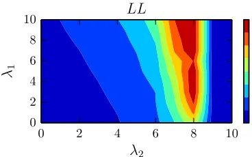
[image:3.612.323.507.68.183.2]LL
Figure 1: TheLLobjective for varyingλ1, λ2.
our approach2 , Skip Gram model is picked as the
baseline. To retain the learning speed, and avoid inctractability of maximum likelihood learning, we learn our embeddings with Noise Contrastive Es-timation using a negative sample (Gutmann and Hyv¨arinen, 2012).
3.1 Model Selection
For model selection, we are going to illustrate the log likelihood of different model instances. How-ever, exact computation of theLL is computation-ally difficult since a full pass over the validation likelihood is time-consuming with millions of sam-ples. Hence, we compute a stochastic likelihood with a few approximation steps. We first subsam-ple a million samsubsam-ples rather than a full evaluation set, and then sample few words to predict in the window context similar to the approach followed in (Levy and Goldberg, 2014). Lastly, we approximate the normalization factor with one negative sample for each prediction score (Mnih and Kavukcuoglu, 2013)(Gutmann and Hyv¨arinen, 2012). Such an approximation works fine and gives smooth error curves. The reported likelihoods are computed by averaging over 5-fold cross validation sets.
Results. Figure 1 shows the likelihood LL ob-tained by varying {λ1, λ2}. The plot shows that
there exits a unique minimum and both constraints contribute to achieve a better likelihood compared to their unregularized counterparts (for whichλ1 =
λ2 = 0). In particular, the regularization imposed by
the differential of context and target embeddingsg2
beddingsΨandΦseparately. This is to be expected
as g2 also incorporates an amount of norm bound
on the vectors. The region where both constraints are employed gives the best results. Observe that we can simply enhance the effect of g2 by adding
a small amount of bounded normg1 constraint in a
stable manner. Doing this with pureg2 is risky
be-cause it is much more sensitive to the selection of λ2. These results suggest that the convex
combina-tion of stable nature ofg1 with potent regularizer of
g2, finally yields comparably better regularization.
3.2 Sensitivity Analysis
In order to test the sensitivity of our model and base-line Skip Gram to variations in the training set, we perform two sensitivity analyses. First, we simu-late a missing data effect by randomly dropping out γ ∈ [0,20]percent of the training set. Under such
a setting, robust models are expected to be effected less from the inherent variation. As an addition, we inspect the effect of varying the minimum cut-off parameter to measure the sensitivity. In this ex-periment, from a classification problem perspective, each instance is a sub-task with different number of classes (words) to predict. Instances with small cut-off introduces classification tasks with very few training samples. This cut-off choice varies in differ-ent studies (Pennington et al., 2014; Mikolov et al., 2013b), and it is usually chosen based on heuristic and storage considerations.
0 5 10 15 20 γ
0.2 0.3 0.4 0.5 0.6
L
L
[image:4.612.324.528.67.185.2]RG SG
Figure 2: Training dropouts effect onLL.
Results. Figure 2 illustrates the likelihood of the Robust and Skip Gram model by varying the dropout ratio on the training set. As the training set shrinks, both models get lowerLL. Nevertheless, likelihood decay of Skip Gram is relatively faster. When20%
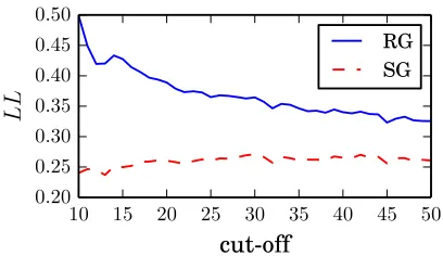
10 15 20 25 30 35 40 45 50
cut-off
0.20 0.25 0.30 0.35 0.40 0.45 0.50
L
L
RG SG
Figure 3:LLw.r.t the cut-off parameter.
drop is applied, the LL drops to 74% in the SG
model. On the other hand the RG model not only starts with a much higher LL, the drop is also to
75.5%, suggesting that RG objective is more
resis-tant to random variations in the training data. Figure 3 shows the results of varying the rare-words cut-off threshold. We observe that the like-lihood obtained by the Skip Gram is consistently lower than that of the Robust Gram. The graph shows that throwing out these rare words helps the objective of SG slightly. But for the Robust Gram re-moving the rare words actually means a significant decrease in useful information, and the performance starts to degrade towards the SG performance. RG avoids the overfitting occurring in SG, but still ex-tracts useful information to improve the generaliza-tion.
3.3 Word Similarity Performance
The work of (Schnabel et al., 2015) demonstrates that intrinsic tasks are a better proxy for measuring the generic quality than extrinsic evaluations. Mo-tivated by this observation, we follow the experi-mental setup of (Schnabel et al., 2015; Agirre et al., 2009), and compare word correlation estimates of each model to human estimated similarities with Spearman’s correlation coefficient. The evaluation is performed on several publicly available word sim-ilarity datasets having different sizes. For datasets having multiple subjects annotating the word simi-larity, we compute the average similarity score from all subjects.
[image:4.612.84.286.487.602.2]Le-bret, 2013) extracts word embeddings by running a Hellinger PCA on the cooccurrence matrix. For this method, context vocabulary upper and lower bound parameters are set to{1,10−5}, as promoted by its author. GLoVe (Pennington et al., 2014) approach formulates a weighted least squares problem to com-bine global statistics of cooccurence and efficiency of window-based approaches. Its objective can be interpreted as an alternative to the cross-entropy loss of Robust Gram. Thexmax, αvalues of the GLoVe
objective is by default set to 100,3/4. Finally, we
also compare to shallow representation learning net-works such as Skip Gram and Continuous Bag of Words (CBoW) (Mikolov et al., 2013a), competitive state of the art window based baselines.
We set equal window size for all these models, and iterate three epochs over the training set. To yield more generality, all results obtained with 300 dimensional embeddings and subsampling parame-ters are set to 0. For Robust Gram approach, we have setλ1, λ2 ={0.3,0.3}. To obtain the similarity
re-sults, we use the finalΦcontext embeddings.
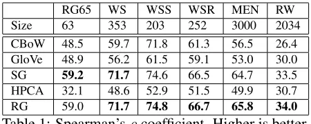
Results. Table 1 depicts the results. The first ob-servation is that in this setting, obtaining word sim-ilarity using HPCA and GLoVe methods are subop-timal. Frankly, we can conjecture that this scarce data regime is not in the favor of the spectral meth-ods such as HPCA. Its poor performance can be at-tributed to its pure geometric reconstruction formu-lation, which runs into difficulties by the amount of inherent noise. Compared to these, CBoW’s perfor-mance is moderate except in the RW dataset where it performs the worst. Secondly, the performance of the SG is relatively better compared to these ap-proaches. Surprisingly, under this small data setting, RG outperforms all of its competitors in all datasets except for RG65, a tiny dataset of 63 words con-taining very common words. It is admissible that RG sacrifices a bit in order to generalize to a large variety of words. Note that it especially wins by a margin in MEN and Rare Words (RW) datasets, having the largest number of similarity query sam-ples. As the number of query samples increases, RG embeddings’ similarity modeling accuracy be-comes clearly perceptible. The promising result Ro-bust Gram achieves in RW dataset also sheds light on why CBoW performed worst on RW: CBOW overfits rapidly confirming the recent studies on the
RG65 WS WSS WSR MEN RW
Size 63 353 203 252 3000 2034
[image:5.612.314.539.56.146.2]CBoW 48.5 59.7 71.8 61.3 56.5 26.4 GloVe 48.9 56.2 61.5 59.1 53.0 30.0 SG 59.2 71.7 74.6 66.5 64.7 33.5 HPCA 32.1 48.6 52.9 51.5 49.9 30.7 RG 59.0 71.7 74.8 66.7 65.8 34.0
Table 1: Spearman’sρcoefficient. Higher is better.
stability of CBoW (Luo et al., 2014). Finally, these word similarity results suggest that RG embeddings can yield much more generality under data scarcity.
4 Conclusion
This paper presents a regularized word embedding approach, called Robust Gram. In this approach, the model complexity is penalized by suppressing de-viations between the embedding spaces of the tar-get and context words. Various experimental results show that RG maintains a robust behaviour under small sample size situations, sample perturbations and it reaches a higher word similarity performance compared to its competitors. The gain from Robust Gram increases notably as diverse test sets are used to measure the word similarity performance.
In future work, by taking advantage of the promis-ing results of Robust Gram, we intend to explore the model’s behaviour in various settings. In particu-lar, we plan to model various corpora, i.e. predictive modeling of sequentially arriving network packages. Another future direction might be encoding avail-able domain knowledge by additional regularization terms, for instance, knowledge on synonyms can be used to reduce the degrees of freedom of the opti-mization. We also plan to enhance the underlying optimization by designing Elastic constraints (Zou and Hastie, 2005) specialized for word embeddings.
Acknowledgments
References
Eneko Agirre, Enrique Alfonseca, Keith Hall, Jana Kravalova, Marius Pas¸ca, and Aitor Soroa. 2009. A study on similarity and relatedness using distributional and wordnet-based approaches. InProceedings of Hu-man Language Technologies: The 2009 Annual Con-ference of the North American Chapter of the Asso-ciation for Computational Linguistics, NAACL ’09, pages 19–27.
Sanjeev Arora, Yuanzhi Li, Yingyu Liang, Tengyu Ma, and Andrej Risteski. 2015. Random walks on context spaces: Towards an explanation of the mysteries of se-mantic word embeddings.CoRR, abs/1502.03520. Sanjeev Arora, Yuanzhi Li, Yingyu Liang, Tengyu Ma,
and Andrej Risteski. 2016. Linear algebraic structure of word senses, with applications to polysemy. CoRR, abs/1601.03764.
Marco Baroni, Georgiana Dinu, and Germ´an Kruszewski. 2014. Don’t count, predict! A systematic compari-son of context-counting vs. context-predicting seman-tic vectors. InProceedings of the 52nd Annual Meet-ing of the Association for Computational LMeet-inguistics, pages 238–247, June.
John Caron. 2000. Experiments with lsa scoring: Opti-mal rank and basis. InProc. of SIAM Computational Information Retrieval Workshop.
Maryam Fazel, Haitham Hindi, and Stephen P. Boyd. 2001. A rank minimization heuristic with application to minimum order system approximation. InIn Pro-ceedings of the 2001 American Control Conference, pages 4734–4739.
Debanjan Ghosh, Weiwei Guo, and Smaranda Muresan. 2015. Sarcastic or not: Word embeddings to predict the literal or sarcastic meaning of words. InEMNLP, pages 1003–1012. The Association for Computational Linguistics.
Amir Globerson, Gal Chechik, Fernando Pereira, and Naftali Tishby. 2007. Euclidean embedding of co-occurrence data. J. Mach. Learn. Res., 8:2265–2295. Michael U. Gutmann and Aapo Hyv¨arinen. 2012.
Noise-contrastive estimation of unnormalized statisti-cal models, with applications to natural image statis-tics. J. Mach. Learn. Res., 13(1):307–361, February. R´emi Lebret and Ronan Lebret. 2013. Word emdeddings
through hellinger PCA. CoRR, abs/1312.5542. Benot Lemaire and Guy Denhire. 2008. Effects of
high-order co-occurrences on word semantic similarities.
CoRR, abs/0804.0143.
Omer Levy and Yoav Goldberg. 2014. Neural word em-bedding as implicit matrix factorization. InAdvances in Neural Information Processing Systems 27, pages 2177–2185.
Qun Luo, Weiran Xu, and Jun Guo. 2014. A study on the cbow model’s overfitting and stability. In Proceed-ings of the 5th International Workshop on Web-scale Knowledge Representation Retrieval & Reason-ing, Web-KR ’14, pages 9–12. ACM.
Andrew L. Maas, Raymond E. Daly, Peter T. Pham, Dan Huang, Andrew Y. Ng, and Christopher Potts. 2011. Learning word vectors for sentiment analysis. In Pro-ceedings of the 49th Annual Meeting of the Associa-tion for ComputaAssocia-tional Linguistics: Human Language Technologies - Volume 1, HLT ’11, pages 142–150. Tomas Mikolov, Kai Chen, Greg Corrado, and Jeffrey
Dean. 2013a. Efficient estimation of word representa-tions in vector space.CoRR, abs/1301.3781.
Tomas Mikolov, Ilya Sutskever, Kai Chen, Greg Cor-rado, and Jeffrey Dean. 2013b. Distributed represen-tations of words and phrases and their compositional-ity.CoRR, abs/1310.4546.
Andriy Mnih and Koray Kavukcuoglu. 2013. Learning word embeddings efficiently with noise-contrastive es-timation. In C. J. C. Burges, L. Bottou, M. Welling, Z. Ghahramani, and K. Q. Weinberger, editors, Ad-vances in Neural Information Processing Systems 26, pages 2265–2273.
Jeffrey Pennington, Richard Socher, and Christopher Manning. 2014. InProceedings of the 2014 Confer-ence on Empirical Methods in Natural Language Pro-cessing (EMNLP), pages 1532–1543, Doha, Qatar. Tobias Schnabel, Igor Labutov, David M. Mimno, and
Thorsten Joachims. 2015. Evaluation methods for un-supervised word embeddings. InEMNLP, pages 298– 307.
Nathan Srebro and Adi Shraibman. 2005. Rank, trace-norm and max-trace-norm. In COLT, volume 3559 of
Lecture Notes in Computer Science, pages 545–560. Springer.
Peter D. Turney and Patrick Pantel. 2010. From fre-quency to meaning: Vector space models of semantics.
J. Artif. Int. Res., 37(1):141–188, January.