A Simple Unsupervised Learner for POS Disambiguation Rules
Given Only a Minimal Lexicon
Qiuye Zhao Mitch Marcus
Dept. of Computer & Information Science University of Pennsylvania
qiuye, [email protected]
Abstract
We propose a new model for unsupervised POS tagging based on linguistic distinc-tions between open and closed-class items. Exploiting notions from current linguis-tic theory, the system uses far less infor-mation than previous systems, far simpler computational methods, and far sparser descriptions in learning contexts. By ap-plying simple language acquisition tech-niques based on counting, the system is given the closed-class lexicon, acquires a large open-class lexicon and then acquires disambiguation rules for both. This sys-tem achieves a 20% error reduction for POS tagging over state-of-the-art unsuper-vised systems tested under the same con-ditions, and achieves comparable accuracy when trained with much less prior infor-mation.
1 Introduction
All recent research on unsupervised tagging, as well as the majority of work on supervised tag-gers, views POS tagging as a sequential labeling problem and treats all POS tags, both closed- and open-class, as roughly equivalent. In this work we explore a different understanding of the tagging problem, viewing it as a process of first identifying functional syntactic contexts, which are flagged by closed-class items, and then using these func-tional contexts to determine the POS labels. This disambiguation model differs from most previous work in three ways: 1) it uses different encod-ings over two distinct domains (roughly open- and closed-class words) with complementary distribu-tion (and so decodes separately); 2) it is determin-istic and 3) it is non-lexicalized. By learning dis-ambiguation models for open- and closed- classes separately, we found that the deterministic, rule-based model can be learned from unannotated data
by a simple strategy of selecting a rule in each ap-propriate context with the highest count.
In contrast to this, most previous work on un-supervised tagging (especially for English) con-centrates on improving the parameter estima-tion techniques for training statistical disambigua-tion models from unannotated data. For exam-ple, (Smith&Eisner, 2005) proposes contrastive estimation (CE) for log-linear models (CRF), achieving the current state-of-the-art performance of 90.4%; (Goldwater&Griffiths, 2007) applies a Bayesian approach to improve maximum-likelihood estimation (MLE) for training genera-tive models (HMM). In the main experiments of both of these papers, the disambiguation model is learned, but the algorithms assume a complete knowledge of the lexicon with all possible tags for each word. In this work, we propose making such a large lexicon unnecessary by learning the bulk of the lexicon along with learning a disambigua-tion model.
Little previous work has been done on this nat-ural and simple idea because the clusters found by previous induction schemes are not in line with the lexical categories that we care about. (Chan, 2008) is perhaps the first with the intention of generat-ing ”a discrete set of clusters.” By applygenerat-ing simi-lar techniques to (Chan, 2008), which we discuss later, we can generate clusters that closely approx-imate the central open-class lexical categories, a major advance, but we still require a closed-class lexicon specifying possible tags for these words. This asymmetry in our lexicon acquisition model conforms with our understanding of natural lan-guage as structured data over two distinct domains with complementary distribution: open-class (lex-ical) and closed-class (functional).
Provided with only a closed-class lexicon of
288words, about0.6%of the full lexicon, the sys-tem acquires a large open-class lexicon and then acquires disambiguation rules for both closed- and
open-class words, achieving a tagging accuracy of
90.6% for a 24k dataset, as high as the current state-of-the-art (90.4%) achieved with a complete dictionary. In the test condition where both algo-rithms are provided with a full lexicon, and are trained and evaluated over the same 96k dataset, we reduce the tagging error by up to20%.
In Section 2 we explain our understanding of the POS tagging problem in detail and define the no-tions of functional context and open- and closed-class elements. Then we will introduce our meth-ods for acquiring the lexicon (Section 3) and learn-ing disambiguation models (Section 4, 5 and 6) step by step. Results are reported in Section 7 fol-lowed by Section 8 which discusses the linguistic motivation behind this work and the simplicity and efficiency of our model.
2 The Tagging Problem
In most work on both unsupervised and supervised problem, tagging is viewed as a sequential label-ing problem. In this work, however, we would like to explore another view on tagging especially con-sidering language as structured data.
The engineering concept of POS tags derives from the linguistic notion of syntactic category which specifies the combinatorial properties of a word in an underlying (syntactic) structure. Given the parse structure for a given word sequence which breaks the input into recursive functional domains such as IP, VP and NP, the POS tag of each word can be directly inferred. Of course, as-suming a pre-parsed structure as input to POS tag-ging is somewhat ridiculous, but it strongly mo-tivates us to highlight the features of structural information for POS tagging. Without resorting to any intermediate representations richer than the input string, we propose for engineering purposes to capture the features of interest for POS tagging by the functional items in language themselves. Then tagging is considered to be a process of iden-tifying the functional contexts (functional items in context) in which the categorical property of the target item can be inferred.
Following ideas in current linguistic theory dis-cussed in Section 8, we observe that the functional categories and some morphological endings serve as markers of the functional domains themselves (discussed above) and sit abstractly at the edge of those domains; the open-class (lexical) items must sit within appropriate functional domains. More
specifically, although long distance dependencies are not at all rare, for a token in sequence, we only consider adjacent closed-class words and the verbal categorical feature (but not morphology) as functional contexts, the core concept in our disam-biguation model.
Our system uses five open-class categories: three basic lexical categories verb, noun and ad-verb, and two derived Nominal categories (the two kinds of participles in English); and consider all other words not included in those categories to be closed-class items.
Overall, for the task of unsupervised tagging, we use a rule-based disambiguation model con-taining disambiguation rules conditioned on func-tional contexts, and the model is learned from unannotated data constrained by much less lexi-cal knowledge than most previous work, namely the closed-class lexicon as introduced below.
2.1 Closed-class Lexicon
A dictionary containing all possible tags for each word is very useful to constrain the unsupervised learning of a POS disambiguation model, and in most previous work, a full lexicon computed from the WSJ corpus (the source of both training and test datasets) is used for both learning and tagging. Since a full lexicon is not a reasonable resource, we aim to limit the required knowledge to func-tional (closed-class) words only.
It is hard to define functional words in a lin-guistically strict sense, but this category is close to the notion within the engineering field of NLP of closed-class words, classes of words that are not open for new members. From the engineer-ing point of view, this implies that a closed class has a finite and static number of members, so its members can be listed once and for all.
For English, lists of closed-class categories such as preposition, pronoun or even degree adverb, are obtainable resources, but this is not necessarily the case for other languages. In this paper, we leave the automatic acquisition of a closed-class lexicon for future work. For experiments in this work, we automatically compute a closed-class lexicon from the WSJ treebank 00-24 sections by picking out those words that are labeled predominantly with closed-class tags1. For each word selected as a
closed-class word, all possible tags encountered 1For each word, if the number of instances labeled by
more than twice in the WSJ corpus are reserved in the closed-class lexicon, so closed-class words may also have open-class tags in our data set, a source of noise in our results. As a core part of language, this closed-class lexicon containing288
entries, about 0.6% of the full lexicon by types, should be invariant over various genres, which is confirmed in experiments on both WSJ and Brown corpus2.
2.2 Tagset
The 45 tags in the Penn Tagset (Marcus et al., 2003) contain more information than just basic lexical categories. In recent work on unsupervised learning of POS taggers following (Smith&Eisner, 2005), the Penn tagset is reduced to 17 tags which nicely improves the tagging performance.
Based on our view of POS tags as local mark-ers of underlying syntactic structure, we derive 27 tags from a feature-based analysis of the original Penn tagset. The main principle for reduction is that we collapse any two tags which are not distguishable by structural features; such features in-clude +/-N, +/-V for predication and +/-wh, +/-en for movement3. For example, under our analysis,
the tag ’VBG’ has the features [+V, +N, tense, -en], tag ’VBD’ [+V, +tense(past), --en], and ’VB’ [+V, -tense(finite), -en]. However, since we do not consider the tense feature to be a structural feature, we do not distinguish ’VBD’ from ’VB’; since N(ominal) is a structural feature, ’VBG’ remains distinct from both ’VBD’ and ’VB’. The 27 tags do not cover all cases of ambiguities of closed-class words in the original Penn tagset. Most no-tably, adjectives are not separated from nouns.
This reduction naturally follows the crucial properties of our disambiguation model. First of all, our model is not lexicalized, so it can only capture basic interactive relations between cate-gories but cannot capture lexical dependencies, which are heavily required to disambiguate ’RP’ 2There are two special classes of words worthy of
dis-cussion with respect to being closed or open. 1. While the morphological ending ’-ly’ freely introduces adverbs, this category is otherwise essentially closed class; and 2. There are obviously unboundedly many numbers(CD), but all these match some regular pattern. So we include adverbs without explicit morphological marking in the closed-class lexicon (we frankly doubt adverbs can be acquired by distributional clustering); and as for numbers, we embed exactly such a regular pattern in our model.
3Not all features of tags are listed here, and further
dis-cussion of the feature-based analysis of the tagset is to be reported in other work. This analysis of tags is motivated by Chomsky.
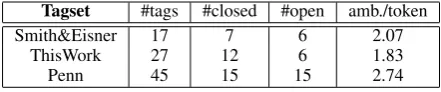
Tagset #tags #closed #open amb./token
Smith&Eisner 17 7 6 2.07
ThisWork 27 12 6 1.83
Penn 45 15 15 2.74
Table 1:Comparison of tagsets
Category Open tags Closed tags
Verbal VB ...
Nominal NN, VBN, VBG DT, CD, PRP($), WDT, WP($)
[image:3.595.306.527.62.108.2]None RB CC, EX, IN, MD, POS, TO
Table 2:N/V categories of 27 POS tags
with ’IN’ or ’PDT’ with ’DT’ (so these two pairs are collapsed). More importantly, the structural information carried by the closed-class items is the key feature of our disambiguation model, but nouns and adjectives are not distinguishable by their structural positions (in NP), so they are not to be distinguished in our tagset4.
We use this new reduced tagset with 27 tags in our experiments5. For the purposes of comparison,
we map the results using our 27 tag tagset to the commonly-used 17 tag tagset6, and evaluate our
algorithms for both tagsets. Table 1 compare the three tagsets, and the ambiguity column shows the average number of ambiguous tags per token in WSJ corpus section 00-24.
2.3 NV category
By using the reduced 27 tags, we found in this work that the heart of the disambiguation task for open-class words is to distinguish them in the Nominal vs. Verbal domains; and for the closed-class words, the Nominal vs. Verbal property of the adjacent context words is also very helpful for
4Due to the indistinguishable roles of adjectives and
nouns in Noun Phrase, it is also hard to extract the adjectives from nouns for lexicon acquisition.
5For open-class categories, we keep VB (for VB*), NN
for (NN*), VBG, VBN and RB (for RB*), and we reduce the JJ* tags to the tag NN and for closed-class tags, we keep al-most all the original distinctions, except for two pairs: ’PDT’ and ’DT’; ’RP’ and ’IN’. Also ’WRB’ is reduced to ’RB’.
6In our tagset, there are two coarser tags which stand for
disambiguation. The Nominal vs. Verbal property is defined through N/V categories of POS tags, and we list each category containing both closed-class and open-class tags in table 2.
3 Acquiring the open-class lexicon
Not being equipped with a full lexicon, our system takes the closed-class lexicon as given, and auto-matically computes possible tags, which must be open class, for all other words in the acquisition process as described below. There are five open-class tags in our reduced tagset, as we describe above: ’VBG’ and ’VBN’ represent two kinds of derived Nominal elements, with correspond-ing morphological endcorrespond-ings attached to the verbal roots; and ’RB’ represents the adverbial class into which new words can only be introduced if affixed with the special ending ’-ly’. Taking into account this special morphology, we divide our construc-tion of the open-class lexicon into two steps: N/V-Clustering and Morphing. At the N/V-clustering step, we classify the base-forms (roots) of open-class words into two clusters in a sparse feature space. At the Morphing step, we count on the em-bedded functional elements (i.e. morphology) to derive specific tags for words in each cluster.
3.1 Clustering
Inducing syntactic categories is a language ac-quisition task on which there has been ex-tensive research, e.g. (Clark, 2003) and (Sch¨utze, 1993), based largely on variants of distributional clustering. In a standard setup of POS clustering, each target word to be clustered, wi, is represented as a vector, <count(wi,C1), count(wi,C2),...,count(wi,Cm)>,
collecting counts of occurrences ofwiin each
con-text, Cj. Then the chosen algorithm clusters the
feature vectors according to similarity.
In previous work, the contextual features are lexical, so the length of a feature vector varies from hundreds to thousands of features. The clustering algorithm then runs over this high-dimensional space, which is computationally quite intensive. Unlike previous work, our system only employs seven features, all functional, to represent target words, and we are paid back by a substantial improvement in efficiency. Each open-class word is represented in the feature space by the following seven component vector:<left:DT, left:MD,
mid:-φ, mid:-ed, mid:-ing, right:DT, right:MD>. The
first two values in this vector represent the counts of modal verbs (MD) and determiners (DT) occur-ring to the left of all forms of a base form; the three values in the middle represent the counts of three possible morphological forms of a word; and the last two values represent the counts of an immedi-ately following MD and DT. This radical reduction of the feature space eliminates any need for so-phisticated clustering techniques. For the purpose of convenience, we use a basic k-means clustering algorithm which allows us to specify the number of output clusters (Maffi, 2007).
As is well known, clustering all words in a cor-pus using distributional clustering results in a high number of clusters. For example, (Sch¨utze, 1993) induces 200 clusters and (Clark, 2003) chooses between 16-128; and most of these induced cate-gories are difficult to associate with a specific POS tag. Chan’s recent thesis work (Chan, 2008) pro-vides us with a solution to this problem. In the first pass of Chan’s model for unsupervised lexical cat-egory induction, verbs are separated from all other categories with a high level of purity; the second pass separates adjectives from nouns by using the categorical results from the first pass as an addi-tional feature7. His experiments for a wide range
of languages show that the ”restriction to clus-ter base forms only8”is crucial to induce clusters
more in line with the definition of the open-class syntactic categories we care about here.
Here, we follow a variant of Chan’s approach, grouping words with their base-forms for cluster-ing. For example, we group all occurrences of the transformed (morphological) forms, (start, starts, starting and started), in a particular context, Cj,
together with the base formstartto form a single count for(start, Cj), in forming the
correspond-ing feature vectors. Given this, since all inflections of one base form share the same feature vector, all inflections enter into the same class of their base-form. In (Chan, 2008), morphological base forms are the output of a new morphology induction al-gorithm he develops. Here, we simply extract the base form of a word by stripping three possible forms of endings:-s,-ingand-ed9.
7For simplicity, we don’t run a second pass but reduce
adjectives to noun.
8See p.139 in (Chan, 2008)
9This simple strategy, as well as more complex
3.2 Morphing
After the clustering step, which we intend to sep-arate the Nominal and Verbal classes, two clusters as desired are induced, but we still need a method to automatically decide which one is which. A trick that works well in practice is simply to pick the smaller class as the Verbal class. These two classes reflect the basic categories of the roots; by a generative mechanism observed in most lan-guages, roots (base-forms) are transformed into derived categories by fusing with functional el-ements, which surface as the few morphological endings in English.
For all words in the Nominal class, except for those with the ending-ly, the only possible tag for each is ’NN’, since no finer categories of ’NN’ ex-ist in our reduced tagset. On the other hand, for a word with ending-ly falling into the N class, we simply assume that its tag must be ’RB’, although this assumption may have a few exceptions.
The Verbal class contains all words with ver-bal roots. There are two specific endings in En-glish serving as morphological markers of derived Nominal categories, -ed and -ing, correspond-ing to derived categories ’VBN’ and ’VBG’ re-spectively. So for each word ending with -ed, we assign two possible tags to it, ’VB’(our re-duced form of ’VBD’) and ’VBN’; and for each word ending with-ing we assume only one pos-sible tag, ’VBG’, although this assumption may systematically introduce tagging error confusing ’VBG’ and ’NN’. For example, if the feature vec-tor representing the base-form groupstart, starts, started,starting is classified into the verbal class, then both starts andstart will receive one possi-ble tag ’VB’;startingwill receive one possible tag ’VBG’; butstarted will receive two possible tags ’VBN’ and ’VB’.
As one may notice,startandstartsshould have two senses, noun and verb, but the Nominal sense is lost in the Morphing step. For such cases, we introduce a simple supplemental process to com-pensate for the missing Nominal sense. For a word with the possible tag ’VB’ (not ’VBG’ or ’VBN’) as determined in the Morphing step, if it is ever seen following a determiner in context, another possible tag ’NN’ will be assigned to it.
Remember that, as introduced in Sect 2.2,
form ofrun, because the ending ’-ed’ is ambiguous for both past tense and past participle. The list of irregular verbs is obtained fromhttp://www.englishpage.com.
’VBN’, ’VBG’ and ’NN’ are of category N and ’VB’ is of category V. Then for each word in the resulting lexicon, there is maximally one possible tag of it falling in either category N or V, so the category information (N or V) is enough for the disambiguation task, as specified in Section 6.
4 Unsupervised Tagging
Taking a dictionary as input, the task of unsuper-vised tagging is to learn a disambiguation model from unannotated data and apply this model for disambiguating the occurrences of words in con-text. In this section, we are going to introduce the representation of our disambiguation model first, and then discuss how it affects the system design. In the following two sections, we will describe the algorithms for learning and decoding the language model respectively.
4.1 Disambiguation Model
Again, we view tagging as a process of identifying functional context, from which the proper tagging simply follows. Given this, we represent the lan-guage model as a set of disambiguation rules con-ditioned on functional contexts that predict cate-gorical information, with each rule of the form of
r = (con : cat) withconandcatthe functional context and categorical information respectively.
In both open- and closed-class domains, given a pair of words (Wl, Wr), the disambiguation
rules check the functional property ofWland
pre-dicts the N/V category of Wr. However, in the
open-class disambiguation model, conrepresents closed-class items as well as verbal feature, but in the closed-class disambiguation model, con rep-resents closed-class categories (closed-class POS tags). In disambiguating an open-class word,con
is checked against the preceding closed-class word or verbal feature (if any), and catof the follow-ing open-class word is predicted. In disambiguat-ing a closed-class wordcw, each possible tag of
closed- class) in context and has a possible tag of ’IN’, then tag it with ’IN’.
This rule-based disambiguation model is deter-ministic in the sense that for each token in context there is maximally one tag that can be predicted. Not being statistically parameterized, this greedy prediction requires that 1) each rule is determistic and 2) in each context, only one rule is in-voked (which is guaranteed by the selection step introduced in Section 5.2). Moreover, this disam-biguation model is non-lexicalized in that it is only conditioned on the functional items in context but not the target word itself.
4.2 System Design
Ideally, we should use closed-class tags in con-text for disambiguating open-class words because closed-class words are potentially ambiguous; but this would cause a chicken-egg problem. If we did this, then the learning of disambiguation rules for closed-class words requires category informa-tion for open-class items and vice versa, but none of the required category information is available from the unannotated data10. Thanks to how
lan-guage works (including principally the low de-gree of ambiguity of closed-class words), it is good enough practically, as shown by our exper-iments, to encode the disambiguation model for open-class words using closed-class items without categorical information.
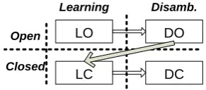
In this way, we can learn the disambiguation model of open-class items from raw data; how-ever, closed-class disambiguation model is better learned after open-class words are disambiguated. Then there are four models in the system for learn-ing and tagglearn-ing over two distinct domains: Model-LC and Model-LO for learning the disambigua-tion model of closed- and open-class words re-spectively; Model-DC and Model-DO for disam-biguating closed- and open-class words respec-tively; and they must be executed in a strict order as follows: Model-LO → Model-DO → Model-LC→Model-DC, as illustrated in Figure 1. 5 Learning Disambiguation Rules
In this section, we describe the learning algorithm used in both Model-LO and Model-LC. Although there is no annotated data available for learning, 10Our disambiguation model is not statistically
parameter-ized, so this problem can not be resolved by any kind of pa-rameter estimation technique as in previous work on unsuper-vised tagging.
Disamb. LO
Learning
LC
DO
DC Open
[image:6.595.340.486.64.128.2]Closed
Figure 1:The order of the four models in system.
we can use the unambiguous events in data to establish the disambiguation rules and apply the rules to ambiguous events. The only difference in implementation of the two models lies in the ’rule-extraction’, corresponding to different interpreta-tions of unambiguous events for learning open-and closed-class disambiguation models. After being extracted from pairs of adjacent words in the input sequence, the rules are counted and selected using the same algorithm in both models.
5.1 Rule-extraction
For open-class words, disambiguation rules are extracted from raw data. A pair of adjacent words
(Wl, Wr) is considered unambiguous if it
satis-fies the following two conditions: 1. Wl is in
the closed class or an unambiguous type with only possible tag of ’VB’; and 2. all possible tags ofWr
fall in the same N/V category (Nominal or Verbal but not mixed). If(Wl, Wr)is unambiguous in this
sense, then extract rule r = (con : cat), where
conisWl(for closed-class words) or ’V’ (for
un-ambiguous verbal words), andcatis the N/V cat-egory ofWr. For example, in the sequence(...he
has claimed..), the pair (he, has)is unambiguous in thathe is a closed-class item andhashas only one possible tag, ’VB’, so a rule ((he : V) is extracted; but (has, claimed) is not usable since claimed has two possible tags: ’VB’ of category V and ’VBN’ of category N.
Disambiguation rules for closed-class words are extracted after open-class disambiguation. A pair of adjacent words (Wl, Wr) is considered
unam-biguous if it satisfies the following two conditions: 1. Wl is in the closed class and has only one
possible tag in the closed-class lexicon; 2. Wr
is either disambiguated or all possible tags ofWr
fall in the same N/V category. If(Wl, Wr)is
un-ambiguous in the above sense, then extract rule
r = (con : cat), where con is the single tag of
Wl, andcatis the N/V category of Wr. For
one possible tag ’IN’ and both possible tags ofhis, ’PRP’ and ’PRP$’, fall into the Nominal category, then a rule(IN :N)is extracted; but(his about) is not usable since his has more than one possi-ble tag andabouthas two possible tags, ’RB’ and ’IN’, which are neither both ’N’ nor both ’V’.
5.2 Counting and Selecting
In the counting step, a set of rulesRis first initial-ized to be empty, and then, as each disambigua-tion ruler is generated while passing through the data, if not already inR, it is added with an ini-tial count of one; otherwise, Nr, the count of r,
is incremented by one. Note that we know that for a rule, (con : cat), the prediction cat can only be either N or V; then for each contextcon, there are two forms of rules counted, (con : N)
or(con:V). By selecting the rule with a greater count for each context, we guarantee that the re-sulting disambiguation model is deterministic.
6 Tagging
Given our rule-based, deterministic language model, tagging is a straightforward process of decoding the disambiguation rules. Recall that there are two separate tagging models in the sys-tem, Model-DO and Model-DC for disambiguat-ing open- and closed-class respectively.
The inputs to Model-DO are the open-class lex-icon, the disambiguation rules learned in Model-LO and raw data in sequence. For each ambiguous open-class word w in sequence if the preceding closed-class word (if any) invokes a disambigua-tion rule,r = (con : cat), then pick the possible tag ofwthat falls in the category ofcat(N or V), as discussed in Section 3.2. If no rule is triggered our default choice is ’NN’; but if ’NN’ is not a pos-sible tag, we assume the default domain is Verbal (so the ‘VB’ tag is favored).
The application of disambiguation rules in Model-DC is a little more complex. For each ambiguous closed-class wordcwin sequence fol-lowed by a token of category cat, N or V, pick a possible tag of cw, con, such that(con : cat)is a rule learned in Model-LC. If no tag is picked, a random choice is made. While there are resid-ual cases that no functional context can help with tagging, the disambiguation model proposed here combined with random choice results in a good overall performance, as shown in section 7.3.
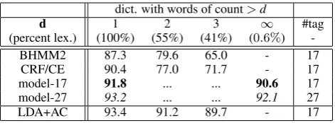
dict. with words of count>d
d 1 2 3 ∞ #tag
(percent lex.) (100%) (55%) (41%) (0.6%)
-BHMM2 87.3 79.6 65.0 - 17
CRF/CE 90.4 77.0 71.7 - 17
model-17 91.8 ... ... 90.6 17
model-27 93.2 ... ... 92.1 27
[image:7.595.307.543.61.148.2]LDA+AC 93.4 91.2 89.7 - 17
Table 3: Tagging accuracy with partial dictionaries over 24k dataset; our closed-class lexicon is the closest approxi-mation to the∞column .
7 Results
Our unsupervised tagging system is com-pared to the following models As reported in (Banko&Moore, 2004), ’the quality of the lexicon made available to unsupervised learner made the greatest difference to tagging accuracy’. So we only compare our experiments to recent work built over the same dataset and a full lexicon automatically extracted from the Penn Treebank. As described in section 2.1, the closed-class lexicon, special in our experiments, is also auto-matically constructed from the WSJ corpus, and will be used in experiments on both WSJ and Brown corpora below11. CRF/CE (Smith&Eisner,
2005) and BHMM2 (Goldwater&Griffiths, 2007) have been discussed briefly in the introduction. LDA+AC (Toutanova&Johnson, 2007) is actually a semi-unsupervised model given the prior on
p(t|w); despite this additional information, our model outperforms it in experiments with partial dictionaries. For the purpose of comparison, our experiments use the same dataset as in these previous work, varying in sizes from 12K to 96K. In addition to reporting on our own tagset with 27 tags, we also map the results onto the 17 tags used in other models as explained above.
7.1 Unsupervised Tagging over Partial Dictionaries
As shown in Table 3, reducing the dictionary by filtering rare words (with count<=d) has not been a promising track to follow for accomplishing the task with as little information as possible. How-ever, by introducing a lexicon acquisition step, we achieve a tagging accuracy of 90.6% for the 24K test data with no prior open-class lexicon, pro-vided with only a minimal lexicon of closed-class items (about0.6%of the full lexicon), as high as 11If we control the quality of the closed-class lexicon (but
size 12K 24k 48k 96K #tag lex.
BHMM2 85.8 84.4 85.7 85.8 17 full
CRF/CE 86.2 88.6 88.4 89.4 17 full
[image:8.595.72.299.62.136.2]Model-17 91.0 91.6 91.6 91.5 17 full Model-27 93.1 93.6 93.5 93.4 27 full model-17 88.9 89.3 90.2 90.4 17 closed model-27 90.9 91.2 92.0 92.2 27 closed
Table 4: Tagging Accuracy of models trained over dataset varying in sizes with full/closed-class lexicon
the best previous performance of90.4given a full lexicon (CRF/CE withd= 1)12.
One other work that investigates the use of a limited lexicon is (Haghighi&Klein, 2006), which develops a prototype-drive approach to propagate the categorical property using distributional simi-larity features; using only three exemplars of each tag, they achieve a tagging accuracy of80.5% us-ing a somewhat larger dataset but also the full Penn tagset, which is much larger.
7.2 Varying in sizes
As shown in Table 4, our new algorithm reduces tagging error by up to 20% over the state-of-the-art given a full lexicon, from89.4%to91.5%over the 96k dataset13.
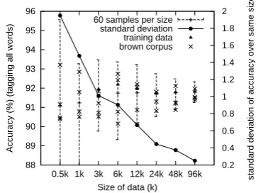
To better understand the learning property of our system and to get an estimate of the vari-ance of our results above, we repeated the exper-iments above, starting with either the full lexicon or just the closed-class lexicon, with datasets vary-ing from 0.5K to 96K in size, and repeated each experiment 60 times on different sequences, with four samples randomly selected from the Brown corpus, one from the training data reported above and the others from the WSJ corpus. As shown in Figure 2, for the closed-class lexicon experiments, the standard deviation of tagging accuracy over the dataset of each size sharply decreases as the size of the data increases, as expected. It is also clear that 12Since we are facing an unsupervised task, the training set
is unannotated, and hence there is no reason not to use it as the test set as well. For the sake of comparison, we use the same split of the dataset for training as previous work. In Table 3 the tagging model is trained over 96k and evaluated on 24k, but in Table 4, the tagging model is trained and evaluated over test and training sets of the same size.
13With a full lexicon, we need to disambiguate between
open-class tags which fall into the same N/V category, which is beyond the ability of our disambiguation rules which pre-dict N or V only. When more than one possible tag in the same category predicted by the disambiguation rule, we sim-ply make a random choice. Although not as constrained as the acquired lexicon, a full lexicon does improve the tagging performance, since the automatic lexicon acquisition is far from perfect.
88 89 90 91 92 93 94 95 96
0.5k 1k 3k 6k 12k 24k 48k 96k 0.2 0.4 0.6 0.8 1 1.2 1.4 1.6 1.8 2
Accuracy (%) (tagging all words)
standard deviation of accuracy over same size
Size of data (k) 60 samples per size
[image:8.595.322.503.80.216.2]standard deviation training data brown corpus
Figure 2: Standard Deviation of Tagging Accuracy with closed-class lexicon; 60 samples for each size, randomly se-lected from both Brown and WSJ corpus.
system with system with closed-class lexicon full lexicon sub-model #errors accuracy #errors accuracy
Model-DO 1089 87.3% 3546 78.9%
Model-DC 1694 89.6% 1709 89.7%
random 1148 44.2% 981 44.9%
recall 3650 - 75
-total 7581 75.2% 6311 82.1%
#ambiguous 30563 35229
Table 5: The number of errors and percentambiguous to-kens tagged correctly in the 96k dataset with 27 tags. For ei-ther system built upon closed-class lexicon or full lexicon, the table shows the disambiguation accuracy and number of er-rors for each sub-model in the system: Model-DO for disam-biguating open-class, Model-DC for disamdisam-biguating Closed-class and random choice. The numbers of recall errors (gold tag not in dictionary) and total errors for each system are also shown.
the performance of our algorithm on the Brown corpus is as strong as on the WSJ corpus. Results for the full-lexicon are similar.
7.3 Error Analysis
There are certainly cases that no functional context can help with tagging, since our disambiguation models are encoded by functional context only. Thus it is worth a closer look to how often the system resorts to random choice, as well as to the disambiguation accuracy of either disambiguation model for open- and closed- class learned from unannotated data. We show the disambiguation accuracy of ambiguous words only for each model in Table 5, and also the number of errors due to imperfect lexicons or random choice.
8 Discussion and Future Work
[image:8.595.306.529.270.366.2]POS disambiguation model. Moreover, the dis-ambiguation model we used is deterministic, non-lexicalized and defined over two distinct do-mains with complementary distribution (open- and closed-class).
Building a lexicon based on induced clusters requires our morphological knowledge of three special endings in English: -ing, -ed and -s; on the other hand, to reduce the feature space used for category induction, we utilize vectors of func-tional features only, exploiting our knowledge of the role of determiners and modal verbs. How-ever, the above information is restricted to the lex-icon acquisition model. Taking a lexlex-icon as in-put, which either consists of a known closed-class lexicon together with an acquired open-class lexi-con or is composed by automatic extraction from the Penn Treebank, we need NO language-specific knowledge for learning the disambiguation model. We would like to point the reader to (Chan, 2008) for more discussion on Category induc-tion14; and discussions below will concentrate on
the proposed disambiguation model.
Current Chomskian theory, developed in the Minimalist Program (MP) (Chomsky, 2006), ar-gues (very roughly speaking) that the syntactic structure of a sentence is built around a scaffold-ing provided by a set of functional elements15.
Each of these provides a large tree fragment (roughly corresponding to what Chomsky calls a phase) that provide the piece parts for full utter-ances. Chomsky observes that when these ments combine, only the very edge of the frag-ments can change and that the internal structure of these fragments is rigid (he labels this observation the Phase Impenetrability Condition, PIC). With the belief in PIC, we propose the concept of func-tional context, in which category property can be determined; also we notice the distinct distribution of the elements (functional) on the edge ofphase and those (lexical) assembled within thephase.
Instead of chasing the highest possible perfor-mance by using the strongest method possible, we wanted to explore how well a deterministic, non-lexicalized model, following certain linguistic in-tuitions, can approach the NLP problem. For the
14In our experiment, using the base-forms and adding a
compensation process improves the coverage rate of the ac-quired lexicon from 79% to 93%.
15Such as determiners (for NPs), complementizers likethat
(for clauses), and case assigning elements associated with transitive verbs (for propositions).
unsupervised tagging task, this simple model, with less than two hundred rules learned, even outper-forms non-deterministic generative models with ten of thousands of parameters.
Another motivation for our pursuit of this deter-ministic, non-lexicalized model is computational efficiency16. It takes less than3 minutestotal for
our model to acquire the lexicon, learn the disam-biguation model, tag raw data and evaluate the out-put for a 96k dataset on a small laptop17. And a
model using only counting and selecting is com-mon in the research field of language acquisition and perhaps more compatible to the way humans process language.
We are certainly aware that our work does not yet address two problems: 1). How the system can be adapted to work for other languages and 2) How to automatically obtain the knowledge of functional elements. We believe that, given the proper understanding of functional elements, our system will be easily adapted to other languages, but we clearly need to test this hypothesis. Also, we are highly interested in completing our system by incorporating the acquisition of functional el-ements. (Chan, 2008) presents an extensive dis-cussion of his work on morphological induction and (Mintz et al., 2002) presents interesting psy-chological experiments we can build on to acquire closed-class words.
9 Acknowledgments
We thank the National Science Foundation for its support of this work under grant IIS-0415138. We greatly appreciate the comments of the anony-mous reviewers; section 7.3 is newly added and two more paragraphs are added to section 2.2 in response to their comments. Also, we would like to thank an anonymous reviewer of a earlier ver-sion of this paper, whose thoughtful suggestion led to a restructuring of the current version. We bene-fited greatly from our discussions with Dr. Charles Yang. Noah Smith provided the data sets and de-tails of the 17 tag tagset used in previous work. Finally, we thank Constantine Lignos for his care-ful editing of earlier versions.
16In some sense, the Minimalist Program was proposed to
explore the idea that the existence of Syntax is especially mo-tivated by efficient language processing.
References
Michele Banko and Robert C. Moore. 2004. Part of speech tagging in context. In COLING, 2004. Erwin Chan. 2008. Structures and distributions in
morphological learning. Ph.D. dissertation, Dept. of Computer and Information Science, UPenn. Alexander Clark. 2003. Combining distributional and
morphological information for part of speech induc-tion. In Proceedings of the 10th Meeting of the EACL.
Chomsky, N. 2006. Approaching UG from below. MIT.
Frank, Robert. 2006. Phase theory and Tree Adjoining Grammar. Lingua.
Sharon Goldwater and Thomas L. Griffiths. 2007. A fully Bayesian approach to unsupervised Part-of-Speech tagging. In Proceedings of ACL.
Haghighi and D. Klein. 2006. Prototype-driven learn-ing for sequence models. In Proceedings of HLT-NAACL.
Kroch, A. and Joshi, A. K. 1985. Linguistic Relevance of Tree Adjoining Grammars. Technical Report MS-CIS-85-18, Department of Computer and Informa-tion Science, University of Pennsylvania.
Charles N. Li, Sandra A. Thompson. Mandarin Chi-nese: A Functional Reference Grammar University of California Press, 1989
Hrafn Loftsson. Tagging Icelandic text: A linguistic rule-based approach Nordic Journal of Linguistics (2008), 31:47-72 Cambridge University Press Leonardo Maffi. Implementation of K-means
cluster-ing in Python.
http://www.fantascienza.net/leonardo/so/kmeans/kmeans.html Mitchell P. Marcus , Mary Ann Marcinkiewicz ,
Beat-rice Santorini, 1993. Building a large annotated cor-pus of English: the Penn Treebank. Computational Linguistics, v.19 n.2, June 1993.
T.H. Mintz, E.L. Newport and T.G. Bever. 2002. The distributional structure of grammatical categories in speech to young children. Cognitive Science 26 (2002), pp. 393C424.
Hinrich Sch¨utze. 1993. Part-of-speech induction from scratch. In Proceedings of the 31st Meeting of the ACL.
Noah A. Smith. Novel Estimation Methods for Un-supervised Discovery of Latent Structure in Natural Language Text. Ph.D. thesis, Johns Hopkins Uni-versity Department of Computer Science, Baltimore, MD, October 2006.
L Shen, G Satta and A Joshi. 2007. Guided Learning for Bidirectional Sequence Classification In Pro-ceedings of ACL.
Noah Smith and Jason Eisner. 2005. Contrastive es-timation: Training log-linear models on unlabeled data.In Proceedings of the 43rd Meeting of the ACL. Kristina Toutanova and Mark Johnson. 2007. A Bayesian LDA-based model for semi-supervised part-of-speech tagging.In NIPS2007.