Online Full Text

Abstract—unlike the trial-and-error as the destiny of simulation, a backward then forward simulation (BFS) technique with multiple-objectives is developed. We apply BFS to a job shop scheduling problem. The objectives are improving utilization of resources and meet the due date commitment of jobs. The system we studied is under incessant input and decision making. And the goal of this research is to derive a real time reflection, stable and controllable dispatching solution with the authentic meaning in practice for real world. In the viewpoint of scheduling technique, we are using the capability and contribution of BFS to reduce the job shop problem into a station of parallel machines scheduling problem. Then, by integrating the decisions over time we achieve the global objectives control. The objectives are utilization and available to promises instate of makespan and tardiness. The discussion in this research is implemented into a system and practice on some reality sites. The related case study report has been accomplished in an accompany paper [1].

I. INTRODUCTION

IMULATION technique was wildly applied as tool for system and design analysis. One of the basic assumption is the simulated system will reach steady state after a proper time. And the goals are bottlenecks, queue length, waiting time etc as terms in queuing theory. In this study we will use simulation as the tool of real time decision making for dispatching and focus on the goal of deliver feasible solution.

The derived solution of traditional technique as discrete event driven simulation is known by the rule base setting and release plan of jobs. Once the factors and release plan in the simulation model are settled then the simulation output will have result without variety. The way to have different results will have to change the factor and release plan in advance then simulate repetitively. Comparing with mathematic programming and scheduling method, the solution of simulation is not derivable by the objective function.

Manuscript received December 22, 2008. The research work was supported by Decision Support Systems Technique Corporation (www.dsst.com.tw) when the first author worked at the institute.

Chueng-Chiu Huang was with Department of Information Management, Tatung University, Taiwan, R.O.C. He is now with the Dept of Industrial Management, Oriental Institute Technology, 58, Sec. 2, Sihchuan Rd., Ban-Chau City, Taipei County 220, Taiwan, R.O.C. (phone: 886-2-89665492; fax: 886-2-77385461; e-mail: fg022@ mail.oit.edu.tw).

Hsi-Kuang Wang is with the Dept of Industrial Management, Oriental Institute Technology, 58, Sec. 2, Sihchuan Rd., Ban-Chau City, Taipei County 220, Taiwan R.O.C. (phone: 886-2-89665492; fax: 886-2-77385461; e-mail: peterwang@ sparqnet.net).

The difficulty of simulation to have objectives derivable solution is due to the unknown future information. Many methods as Simulated Annealing, Gene Algorithm, Ant Colonics, and Forward then Step Back are applied for solving the problem of deriving a solution by objectives. Basically, these trials are all making decision based on the information on hand, and the derived solution is ambiguous in contributing to the objectives.

With the evolution of computer era, the performance of simulation provides much more detail information in efficient way, and then changes the purpose of applying simulation. One of the most important usages becomes connecting the real time information into the simulation system to create instant solution for execution (real time dispatching). In other words, the efficiency of hardware and software extends the purpose of using simulation from solving the plan level issues to execution level.

Basically there are three techniques for modeling decision problem in using the future information. The first is by the statistics skill based on the history data. The second is using mathematic programming by given the coefficients, where the data of coefficient might be derived by history data or judgment. The third is applying simulation model with known arguments. In this study we focus on the discussion on simulation models, precisely, the modified backward then forward simulation to have the result for execution control purpose.

We start the discussion on a transit simulation model with roll back. The idea is setting some barrier states or index in the simulation model, for example the maximum waiting number of jobs or time in queue or tardiness limit of jobs. When simulation is performed and reaches the barrier condition, it will be rewired to earlier stage with modified state arguments for controlling purpose. A usual drawback of the forward then step back method is that there is no guaranty that the simulation will converge to the desired range of the objectives and complete the trial by avoiding the deadlock situation in the decision process.

The backward then forward simulation we proposed in this study is similar to Kim [3], Mejtsky [4], and Watson [5]. In backward, the events are executed from the future to now, so that it might have the future information to be transferred back to earlier decision stage. And the information of later stage from backward will be used for decision making in forward simulation at earlier stage. We will give a clear definition and the functionalities of the backward/forward simulation model that might have the objective control, manage on execution level as connecting the real time

Backward Simulation with Multiple Objectives Control

Chueng-Chiu Huang and Hsi-Kuang Wang

information and then provide a stable solution.

In the following of this article, we have discussion of the intention of the backward simulation in section 2. In section 3, we expound the objectives of utilization and due date commitment. And in section 4, we condense the job shop scheduling problem into a single station with parallel unrelated machines problem, which via the embedded data from backward to achieve the multi-objective of job shop circumstance. The conclusion and study for future research will be in section 5.

II. THE INTENTION OF BACKWARD SIMULATION Backward simulation is applying the event driven sense as regular simulation does, from future to pass or from the right to the left on time line, Watson, Medeiros, and Sadowski [5]. It is trivial that the backward simulation might be performed as well as forward when there is no probabilities condition in the routing for jobs and the capacity availability on time.

Usually the solution derived from backward is neither a suitable result for balance controlling of the resources utilization nor for bottleneck analyzing, and is an illogical application for the material requirement plan. When simulation is performed in backward, we have the solution of exercising the operation as late as possible. The system will also derive results as bottleneck and traffic jam in backward sense. Engaged with the backward, we have forward simulation which applies the solution (operation sequence on machines) from backward; these operations will be performed in non-delay or left-shift sense. The bottleneck and traffic jam of forward will be different from the backward with great chance. For the manner of backward, whenever an operation of a job is selected first for allocating resource prior to the others, it indicates the operation will be performed later. Follow up with the forward simulation, a left-shift is applied.

We note that the state of affair is acceptable for capacity allocation of resource but not for material. We shall give the dissimilarity of resource and material. Material has property as deferability but capacity doesn’t. The resource allocation might be performed in either left- or right- shift but material can’t. Thus when backward simulation had situation as lack of material in a decision; and we had the inventory allocated to the later operation but an earlier one with same priority. Usually, the materials should fulfill the earlier operation but the later ones. And the material allocation conflict in backward and forward caused a complicated solution revise.

Intuitively, backward simulation starts at the last operation’s completion time for each job by its due date, that is, backward will start with the objective of zero tardiness Mejtsky [4]. An operation is ascertained when the service request by job and the effort support by resource were matching. Simulation in backward or forward records the dispatching of job and resource on each operation. The recorded detail information includes the start and completion times of each operation for all jobs and the sequences of

operations for the resources. These are two basic Gantt charts; Job-Time view and Resource-Time View; and shall be discussed in section 3.

A left-shift policy is performing forward simulation by keeping the sequence of these operations on each resource derived from backward. In this manner, when the latest release time of operation I of job j, rij is later than the current time tnow, and then the objective of zero tardiness will hold, Mejtsky [4]. In case of the latest release time is earlier than the current time, rij < tnow, and then the current solution shall have tardiness great than zero. We might have situation as the operations do not follow the sequence to appear at resources, even though we release jobs as the schedule derived in backward. When resource is available, the non-delay policy will let the appeared operation be executed on the resource ignoring the order derived in backward. Thus we might have the improvement of the utilization locally but have no guaranty to the utilization in global and to the tardiness over the time.

In backward scheduling, the due date of each job is used as the release date in forward, and all the other provisions are keeping alike. Kim studied simulation for parallel machines and job shop with the objective of minimizing makespan Kim [3]. He used the backward result in the followed forward schedule by keeping the ordered sequence under left-shift sense. Mejtsky found the solution derived by backward is better than forward on the objective of minimizing makespan for job shop with small size example Mejtsky [4]. However, it shows backward scheduling might provide a new vision of the scheduling problem but for optimizing the objectives as due date and utilization related. There is no proof that backward will provide better solution than forward.

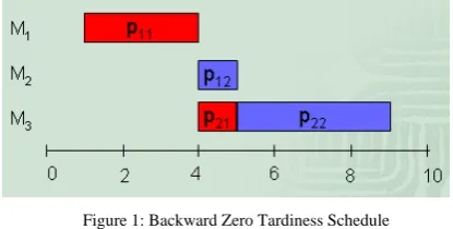
We give a simple and clear explanation to show for keeping the backward result in forward scheduling with left-shift policy will usually not be an acceptable solution. For example, gives jobs J1 and J2 and machines M1, M2, and M3.

Job 1 will be processed on machine M1 then M3, with

processing time p11 = 3, p21 = 1, where pij denotes the processing time of job j on operation i. Job J2 will go thru

machine M2 then M3, and p12= 1, p22 = 4. The due date of job 1 and 2 are d1 = 6, d2 = 9. We have the backward scheduled result with zero tardiness as shown in Figure 1.

Figure 1: Backward Zero Tardiness Schedule

Figure 2: Left-Shift Result by the sequence from Backward Schedule

The result shows the objective of zero tardiness is kept, but the solution is not acceptable when comparing with the following schedule shown in Figure 3.

Figure 3: Non-Delay Forward Schedule

In Figure 3, the operation 2 of job 2 is processed on machine M3 from time 1 to 5. It is a cut-in activity by the

non-delay policy. The activity contributes shorter makespan but has no improvement neither worse to the objective of tardiness. Comparing the results of Figure 2 and 3, we found if the due date of job 1, d1 is earlier then 6, then the result of Figure 2 will turn to be a desired solution. It is due to the tardiness will be keep at zero. On the other hand, if d1 is later than 6, then the schedule of Figure 3 is expected. Therefore, we applied a backward solution in forward either by left-shift or non-delay will depend on the situation for reasonable consideration. That is when the result comes out with zero tardiness committed, then, we might choice a solution with shorter makespan. Otherwise, we might have a solution with longer makespan but the zero tardiness is achieved. We note that if the latest release time obtained from backward is later than time zero, then the acceptable solution will be as shown in Figure 2. And, if it is earlier than time 0, then solution in Figure 3 is a reasonable one to be chosen. When the situation that zero tardiness cannot be achieved in any feasible solution, then which solution is preferred will be an issue for study in practice. However, when we set the processing time of operation 2 for job 2 to be less than 2, p’22 <= 2, then we shall have the result as cut-in or non-delay, as shown in Figure 4, the latest release time will have no effect to the schedule.

Figure 4: A Cut-In result with no effect on the tardiness objective

We note that if minimizing makespan is the major target of the objectives, then non-delay policy for the forward is analogous to the backward. When one considers the due date related objective such as lateness, tardiness or tardy jobs then the cut-in activity of non-delay policy might derive an illogical solution depend on the decision making time and the data comparing with the right-shift policy.

With the above discussion, we might conclude that the purpose of performing backward simulation is for the scheduling purpose. Precisely, the backward then forward scheduling is progressed for conjugating the real time information acquired from shop floor information system in execution level with the information as master planning in plan level. The reason for backward/forward scheduling is not suitable for providing a planning level solution is same as the regular scheduling in forward only. That is they are all using the processing time and performed on time line as simulation does. In this manner, the solution is in detail level as shown in Gantt chart phenomenon; every machine and operation of job have their start and finish times. Usually, the solution for planning level is in time bucket sense that is the capacities of resources and planned quantities to be produced in month, week, day, or hour.

III. THE OBJECTIVES OF UTLIZATION AND DUE DATE COMMITMENT

There were many research analyzed job shop scheduling problem with bi-objectives of minimizing tardiness and makespan. Zero tardiness is an intuitive objective considered at the very first step starting with the backward scheduling. As discussed in section 2, the derived result in backward with the scheduled start time sij, and completion time cij for all the operation i of job j, has to conjugate with the current time and the concurrent situation. The conjugation will turn to be extremely difficult when there are some operations in progressing on certain resources at certain time, and then it is not just simple as left-shift or non-delay activity can support to fit in.

As shown in the following Figure 5, we have a 3 Axis Gantt chart formed by time, machines (resources), and orders (jobs) axis.

Figure 5: 3 Axis Gantt Chart

Each one three-dimensional block in the 3-Axis Gantt chart denotes an operation of a job processed on a resource with certain time period. 3-Axis Gantt chart is derived from an ordinary production control chart used by most of the manufacturing plants. A production control chart is formed by jobs list in the vertical axle and processing stages in the horizon axle. At the cross position of production control chart, a quantity denotes the amount of the job at the stage when it is recorded. The purpose of constructing the control chart is to monitor the progress for each job. We modify the axle of stages into machines or resources, and put these charts together in order of the recorded time, a time axle is formed, and then we have the 3-Axis Gantt chart.

We express the 3 Axis Gantt chart into two categories as Machine_Time and Job_Time, as shown in the following Figure 6:

Figure 6: Machine_Time and Job_Time Gantt Chart

In Figure 6, we can see these jobs are processed on each machine in order as its routing. And the machines progress these operations for each jobs in order of their availability and maybe the dispatching rule too. For example, the sequence of J2 in Figure 6 starts at M4, then will go thru M3, M1, and

finally to M2. For M2, it will process the operations of O41,

O12, O32, and then O24 in ordered too.

We shall focus at the disconnected space between these adjacent two blocks in Machine_Time and Job_Time Gantt chart. These are the idle times or waiting times for machines and jobs. From the Machine_Time chart, the idle time of machine states machine waited for job. Similarly, for the Job_Time chart, the space denotes the job waited in queue for the service from machine. The techniques and solutions for managing these idle times are exactly the issues for most of the problems in real world and researches in academic.

From the view point of these two categories, the idle/waiting times happen independently. Usually minimizing the idle time for machine or for job is handled under different objectives all alone. For example, the productions engineers will endeavor to minimize the idle time for machines, so that to reach the highest performance of utilization. In academic research, minimizing the makespan is a comparable objective of increasing utilization. On the other hand, from the view point of Job_Time chart, minimizing the lead time is an operational target in common sense. Precisely the objective of minimizing lead time is translated into a due date related control goal. Thus giving and practicing due dates with the job release date and lead time control are the management objectives for sales and planners as their customer service performance.

However, by the expression of 3-Axis Gantt chart, we know the idle/waiting times in the two categories are strongly connected with each others. Whenever a decision is made for shrinking the idle space for machine, increasing its utilization, we shall find there is a strong dependency with the operation sequence among these jobs. That is the decision activity might cause a damage to the due date commitment for other jobs with their completion times. For example, in order to save the setup time, the scheduler might put a job with later due date in processing before an urgent one which needs a setup on the resource. Similarly, the activities of shrinking waiting time for jobs have strong dependency with the dispatch for these jobs queuing before machines. Usually, the activity of reducing the job’s waiting time will downgrade the utilization of the resources. For example, the planner put more hot lots in system with shorter lead time, and then more interruptions will occur on resources.

Usually, an objective as due date commitment is a trivial objective but the lead time reduction is not. Similarly, to minimize the makespan is not easily to be translated into increase the utilization of resources. We shall deduce the due date commitment from the lead time control in the following discussion of minimizing makespan and zero tardiness with example. Suppose we have 2 jobs J1, J2 processed on 2

from time 10 and schedule these operations in backward to obtain the completion C1 = 6, C2 = 10. Thus, the tardiness for job 1 and 2 are T1 = (6 - 8)+ = 0, T2 = (10 - 12)+ = 0, and the makespan Cmax = 10 – 1 = 9. The start time of the first operation is at time 1, the completion time of the last operation is at time 10.

Figure 7: Backward Schedule under zero tardiness

Based on the result of Backward (BW), we apply Left-Shift activity to obtain the forward results with makespan remaining Cmax= 9, and T1 = T2= 0, as shown in Figure 8.

Figure 8: Forward schedule by Left-Shift under BW The result shown in Figure 8 is one of the optimal solution for tardiness, but not an optimal solution for makespan. By swapping the order of J1 and J2, we obtain the same result as minimizing tardiness T1 = T2 = 0, and Cmax= 6, the result is shown in Figure 9.

Figure 9: Forward schedule by Swapping J1 and J2

For a further discussion, we assume the available time for M1 is shift from time 0 to time 3. Then by the schedule of

Figure 9, we have a result shown in Figure 10.

Figure 10: Forward schedule

The makespan remains 6, but the tardiness changes T1 = 1, and T2 = 0. Let the schedule change back to same as in Figure 7 with the available time of M1 at time 3, then we have T1 = T2 = 0, Cmax= 9, as shown in Figure 11.

Figure 11: Forward schedule

From the above discussion, we found the decision might be opposite which depend on the time when it is made. A cineraria as the decision maker will give different judgment depend on the time with all the circumstances condition exactly same. In practice, a decision maker will try to meet the due date requirement then consider to improve the utilization of resource, or he/she must decide which objective should be fulfilled with priority.

A regular approach to handle the bi-objective problem is by giving the different objective with a weight respectively. The author will admit the approach of giving weight to different objective is suitable for research but not in real world. In practice, the weight is full of variety by the combinatorial situation of jobs and machines, and most of all, the weight will be different by the factor of time. Thus in the decision process sense, we will give resolution following the time line in a simulation when a decision event happened. The criteria of minimizing makespan or meet due date for a decision making is based on the activity to decide the idle or waiting time for a job or machine should it be saved or sacrificed. With the results accumulated from the decisions process via time line, we might perform in forward and similarly in backward, to minimize the tardiness and then increase the utilization.

4. BUILDING JOB SHOP DECISION PROCESS BY A GROUP OF STATIONS WITH PARALLEL MACHINES

Following with the objectives and decision activities discussed in previous section, we have to make a sequence of decisions along the time line as event driven did to achieve the global objectives of minimizing the tardiness for jobs and maximizing the utilization for resources. Since the decision is made when an event happened for an operation of job and a resource or a material become available, then a decision have to be made for matching with the consideration of increasing utilization and meeting due date.

were applied in many research too. Most of all, they are simulation base. However, these approaches still cannot derive solution driven by the objectives.

Backward approach shows the anticipation of accomplishing the objective of zero tardiness and minimum makespan by the sequence combination of these operations creating in backward. Apart from the objective of tardiness and makespan, we apply the backward capability as simulation, and use these data created in backward simulation, namely the start and completion times, sij, dij, for each operation in forward scheduling manner. That is when a decision had to be made at an event, the system will use the information of Oij; the operation i of job j; in detail level as the release time rij, and due date dij, where

rij = f(ci-1j),

dij = g(si+1j).

The release time rij of Oij is a function of the completion time ci-1j of Oi-1j, which is the previous operation’s completion time. Similarly, the due date dij is a function of si+1j, which is the start time of Oi+1j. We note that different jobs might have exactly same release and due dates at job level, which is due to they are all derived from same sales order and product item, but the release and due dates for operation level will not be same. And the difference is caused by the limited capacities of resource and or the availability of material, then formed the sequence of the operations.

Consider a decision is making when an event occurred, the system will have to judge the suitable match for resources with operations, and take left-shift or non-delay activity by the situation of the operations and resources at the decision moment. The consideration for the decision is described as in previous section that is the utilization and completion time of the operation related to its due date. However, the contribution of the utilization improvement or sacrifice for due date fulfillment suit with the operation but the job itself. It is not trivial for a decision making contributes to the job due date and the overall utilization of the resources in system. Recalled the information of release, start, and due date for every operation which presents the complex connection and relation between resources and operations of the jobs. With the information in detail level, thus a decision is made for operations under the circumstance of parallel machines in a single station, and we might have the result connecting to the due date of jobs and utilization to the resources.

We note that the cycle time control for an operation of a job at a station in practice is exactly implementing the same idea of reduction the control of job shop into a parallel machines problem.

IV. CONCLUSION AND FUTURE STUDIES Objectives derivable simulation architecture in backward then forward sense is provided. In the viewpoint of scheduling technique, it is using the capability and contribution of backward then forward simulation to reduce

the job shop problem into a station of parallel machines scheduling problem. Then, by integrating the decisions over time line it achieves the global objectives control. The objectives are utilization and available to promises but makespan and tardiness. The discussion in this research is implemented into a system and practice on some reality sites. The related case study report has been accomplished in an accompany paper, Wang & Huang [1].

More discussion is needed for future studies. The topics include:

1) The conjugation of the real time information of these operations in WIP status with the solution generated by system.

2) The generation of a solution with controllable stability. Usually, a solution generated by mathematic programming is an unstable one. The solution generated by simulation has same issue of unstable.

3) The chosen of start time in the backward will need more understanding of the meaning. That is the appositive of the release time for forward.

It is a territory of computer simulation for production scheduling close to the execution level but the legacy analyzing for steady state of the system in planning level. And then the objectives of makespan and tardiness have to be modified from jobs view into time horizon view that is the utilization and ATP. Moreover, the author believes the business process build upon the cycle time control might have to be modified as the completion time control for operation.

ACKNOWLEDGMENT

Thank Decision Support Systems Technique Corporation

(www.dsst.com.tw) when the authors worked at the institute.

The technique results are mostly embedded and demonstrated in the scheduling system namely Advance Factory System (AFS). AFS is currently endorsed in IC and MEMS foundry, and PCB factory.

REFERENCES

[1] H-K, Wang and C-C, Huang, “An Analysis of Supply Chain Solution Techniques for IC Production”, IAENG ICINDE2009,, submitted for publication.

[2] Goadratt , “Necessary, but not Sufficient”, 2002.

[3] Y-D. Kim, “A Backward Approach in List Scheduling Algorithms for Multi-Machine Tardiness Problems”, Computer Operations Research, Vol. 22, No. 3, pp. 307-319, 1995.

[4] G. Mejtsky, “Backward Simulation and Multiple-Objective Optimization of Job Shop Scheduling with Zero Tardiness and Minimum Makespan”, Proceeding of the 1985 Winter Simulation Conference, 1997, pp. 716-720.