Inferential Estimation for a Ternary Batch Distillation

Inferential Estimation for a Ternary Batch Distillation

P. Kaewpradit, P. Kittisupakornand I. M. Mujtaba

Abstract—A Kalman filter (KF) estimator has been formulated using a sequence of reduced-order models representing a whole batch behavior for providing the estimates of dynamic composition in a ternary batch distillation process operated in an optimal-reflux policy. A set of full-order models is firstly obtained by linearizing around different pseudo-steady state operating conditions along batch optimal profiles. They are further reduced their orders to achieve their observability and controllability individually by using a model reduction method. The performances of the reduced-estimator have been investigated and compared with those of a conventional nonlinear estimator. Simulation results have demonstrated that the performances of the proposed estimator are reasonably good and almost identical to the conventional one in all cases.

Index Terms—Batch distillation, Kalman filter (KF), Inferential estimation, Model reduction.

I. INTRODUCTION

Batch distillation is an important unit operation widely used in fine chemistry, pharmaceutical, biochemical and food industries to process small amounts of materials with high added value. The main reason is its operational flexibility that a single column can separate all components of a multi-component mixture into several products within a single operation. So as to meet product specification, the batch column needs to be operated as precisely as possible.

If instant compositions are known, an automatic closed-loop control scheme can be implemented correctly to drive the process to the desired operating strategy. However, an online composition analyzer is not economical. Furthermore, it usually introduces a large time-delay into the control loop. Otherwise real-time composition concentration can be estimated from available temperature measurements using an inferential composition estimator.

Manuscript received April 1, 2008. This work was financial supported from the Thailand Research Fund through the Royal Golden Jubilee Ph.D. Program (Grant No. PHD/0204/2546).

P. Kaewpradit has graduated her doctoral degree in 2007 from Department of Chemical Engineering, Chulalongkorn University, Bangkok 10330, Thailand (e-mail: [email protected]).

Assoc. Prof. P. Kittisupakorn is with Department of Chemical Engineering, Chulalongkorn University, Bangkok 10330, Thailand (corresponding author to provide phone: 218-6892; fax: +66-02-218-6877; e-mail: [email protected]).

Prof. I. M. Mujtaba is with School of Engineering, Design and Technology, Bradford University, EDT 3, West Yorkshire BD7 1DP, UK (e-mail: [email protected]).

The use of the estimator has long been suggested to assist monitoring and control of a continuous distillation [1] – [3]. Conversely to the batch column, the issue has received little attention. An Extended Luenberger Observer (ELO) was primarily applied to a multi-component batch system through the use of the tray temperature measurements [4], [5]. As the observer was based on a deterministic model and its gains were obtained in off-line fashion, its performance was degraded rapidly when the measurements were affected by noise.

Therefore, use of a stochastic estimator like a Kalman Filter (KF) was recommended if large amount of noise is expected [6]. Afterward a discrete Extended Kalman Filter (EKF) for the conventional batch distillation was developed to handle the effect of noise by [7]. Recently, [8], [9] have applied the EKF scheme for the composition estimation in a batch reactive distillation.

Even though the EKF is much more robust to mismatch and noise than the ELO, but it is rather difficult to initialize all states and requires considerable computational effort for online use due to model complexity. Furthermore its performance heavily depends on the thermodynamic modeling of vapor-liquid equilibria.

In practical point of view, this work develops a linear-version of the KF estimator using multiple reduced-models sequentially, and implements to the conventional ternary batch column for estimating the product composition profiles.

II. ATERNARYBATCHDISTILLATION In a conventional batch distillation, a liquid mixture is charged into a vessel and heat is added to produce vapor fed into a rectifying column. A concentration of the lightest component increases in the upper trays sequentially in the column and a concentration of a subsequent heavy component increases in a still pot. As the concentration of the lightest component in the distillate reaches its specified purity level or the unit in total reflux operation is taken to a steady state, the distillate product withdrawal is then begun.

The equations describing the process are given below. More detailed description of the operation and modeling of the batch column are referred to [10], [11].

(

)

(

1i 1i

)

1 1 i 1 i , 2 1 2 i

1 _{y x}

H V x x H L

dt dx

− −

−

= (1)

(

)

(

(

)

1 1l

)

l 1 l 2 2 R l 1 v 1

1 Q L h h H h

h h

1

V + − − δ

−

= (2)

(

)

(

j1,i ji

)

j 1 j ji i , 1 j

j 1 j ji

x y H V x x H L

dt dx

− +

−

= − ₋

+ +

(

ji ji

)

j j x y H V −

− (3)

j j 1 j 1 j

j L V V H

L = + + − − −δ (4)

(

)

(

(

)

(

lj

)

)

v 1 j 1 j L j l 1 j 1 j l j v j

j L h h V h h

h h

1

V − + −

−

= + + − −

(

l

)(

j lj

)

j v j h H h h 1 δ − − (5)

(

N 1i Ni

)

N 1 N Ni x y H V dt dx − = − ₋ (6) N 1 N

C V H

L = ₋ −δ (7)

(

)

l

N N l N v 1 N 1 N

C V h h H h

Q = _{− −} − − δ (8)

where, LN =rLC. Change rates of molar holdup and liquid

enthalpy are approximated by using a first order euler integrating approach. Reboiler holdup at any time is calculated from the following algebraic combination,

k , a N 2 j k , j k ,

1 B H H

H _⎟⎟−

⎠ ⎞ ⎜⎜ ⎝ ⎛ − =

∑

=

ο (9)

Antoine’s equations are used in a bubble-point calculation, and both liquid and vapor enthalpies are obtained from experimental correlations [12], [13]. The variation of liquid density is described by using a modified Rackett equation. Column specification used in this study is given in Table I.

III. EXTENDED KALMAN FILTER (EKF)

A. Algorithm of the estimator

A nonlinear process can be described by following differential and measurement equations:

(

x,u

)

w f

x&= +

( )

x v h

y= + (10)

where w and v are vectors of process and measurement noises respectively with covariance Q and R respectively.

Corrected estimates are computed as a linear combination of priori estimates and a weighted difference between actual and predicted measurements:

(

)

(

k kk 1

)

k , est 1 k k k k x ~ h y K xˆ x ~ − − + −

= (11)

1 k k k k , est 1 k k k

k =Σ − −K H Σ −

Σ (12)

where,

(

k kk1 kT

)

1

T k 1 k k k ,

est H H H R

K =Σ ₋ Σ ₋ + − is an

estimator gain and

( )

1 k k xˆ k x x h H − ⎟ ⎠ ⎞ ⎜ ⎝ ⎛ ∂ ∂ = .

[image:2.595.57.280.81.266.2]

For a prediction step, the estimates for the next time step are predicted based the current estimates in which the discrete prediction equations are employed:

Table I: Column specification

(

kk k

)

k 1

k x ,u

~ f x ~ ₌ + (13) Q F Fk kk kT k

1

k = Σ +

Σ ₊ (14)

where,

(

)

k u , k k xˆ k x u , x f F _⎟⎟ ⎠ ⎞ ⎜⎜ ⎝ ⎛ ∂ ∂ = .

B. Application to a batch distillation

As the nonlinear estimator based rigorous mathematical model of an actual plant is rather complex, a simplified model integrated with a bubble-point calculation is easier to be employed in practices. The simplified equations are given by:

(

)

(

1i 1i

)

1 i 1 i 2 1 i 1 x y H V x x H rV dt dx − − −

= (15)

(

)

(

j1,i ji

)

j ji i , 1 j j ji x x H rV y y H V dt dx − + −

= _{− +} (16)

(

N1,i Ni

)

N Ni x y H V dt dx −

= ₋ (17)

At each integration step in an EKF scheme, a reboiler holdup prediction is obtained as,

(

)

j N a,k

0 k ,

1 B N 2 H H H

H = − − × − −

where H_a,k =H_a,k−1 +Δt×

[

(

1−r

)

V

]

. In this case, a state vector is

[

x11,x21,...,xN1,x12,x22,...,xN2

]

T in which

only first two components are considered.

The heaviest component can be obtained by subtracting the summation of the first two components from one. The measurement equations are derived from Antoine’s equations. From (15) – (17), the knowledge of H , j HNand

In the work of [7], the instant vapor flow rate is estimated by the knowledge of vaporization heat and heating power. Nevertheless the exact calculation of the heat of vaporization is difficult then the assumption of the constant vapor load along the batch is made here. The constant values of the parameters Hj,HN, and V are obtained in an

optimal manner as 0.0052 kmol, 0.0427 kmol and 1.4195 kmol/hr respectively.

IV. INFERENTIAL MODEL DEVELOPMENT

However, the use of the nonlinear estimator for estimating product compositions presents two main difficulties:

• The precise estimates of all column-compositions (states) are required. This introduces a difficulty of estimator tuning and poor estimation performance due to un-satisfaction of state-observability.

• Commonly the batch distillation is a large system according to the number of components and plates. Relative computation effort is then required for estimating the states due to complexity and enormous size of the model.

To overcome those, building inferential model for a kalman filter (KF) design using a model reduction approach is presented next.

A. Reducing models through a model reduction

A linear version of (10) can be obtained by linearizing the equations around the reference predefined trajectories as following,

Bu Ax

x&= + (18a)

x C

ym = m (18b)

x C

yum = um (18c)

where, x∈ℜnx , u∈ℜnu denote system states and

manipulated input vectors, and ym∈ℜnym and

nyum um

y ∈ℜ are vectors of (secondary) measurable and (primary) un-measurable outputs.

In most cases, a full-local model contains additional unobservable and/or uncontrollable states. However, only observable and controllable states are needed for a monitoring and control. In this study, a reduced-model is obtained by applying the following steps: (I) system diagonalization, (II) stable-unstable decomposition, (III) gramian balance, (IV) balanced-state truncation, and (V) stable-unstable combination [14].

By applying those steps to the observable system (18a,b), the equations in the reduced-state domain (xr ∈ℜnr) can be formulated as,

u B x A

x&r = r r + r (19a)

r mr m

x C

y = (19b)

where, nrnr

u nrs nrs s

r

A 0

0 A

A × ∈ℜ ×

⎥ ⎥ ⎦ ⎤ ⎢

⎢ ⎣ ⎡ =

nu nr

u nu nrs s r

B B

B × ∈ℜ ×

⎥ ⎥ ⎦ ⎤ ⎢

⎢ ⎣ ⎡ =

nr nym mu

nrs nym ms mr

C C

C ×

× ⎥⎦ ∈ℜ

⎤ ⎢⎣

⎡ =

in which, the matrices in a stable part are

(

1

)

1 nxsnxs

s

A

A =ϑ⋅ ς− ⋅ ⋅ς −⋅ϑ− ∈ℜ ×

(

1

)

nxsnu

s

B

B =ϑ⋅ ς− ⋅ − ∈ℜ ×

(

m

)

1 nymnxs

ms

C

C = ⋅ς − ⋅ϑ − ∈ℜ ×

and the matrices in an unstable part are

(

1

)

nxunxu

u

A

A = ς− ⋅ ⋅ς +∈ℜ ×

(

1

)

nxunu

u

B

B = ς− ⋅ + ∈ℜ ×

(

m

)

nymnxu

mu

C

C = ⋅ς +∈ℜ ×

Similar diagonal system is firstly determined by multiplying with a transform matrix ς (or eigenvector of the corresponding matrix A) for simply identifying the stable and unstable parts of the system. It is noted that the matrix

(

ς−1⋅A ⋅ς

)

is diagonal, in which its elements are eigenvalues of the matrix A . The symbols

( ) ( )

. +, . − denote positive (unstable part) and negative (stable part) eigenvalues respectively.

Afterward the stable part of the similar diagonal system is reduced its dimension by using the balance truncation approach. Observability and controllability grammians are balanced by multiplying a transform matrix ϑ. Less observable and controllable states are further truncated, in which the symbol, ._nrs×nrs, denotes the matrix that only first (nrs) rows and (nrs) columns are considered.

Lastly the reduced stable and unstable parts are composed to preserve the major characteristic of the system. The reduced-order (nr) is then a combination of a reduced-order of the stable part (nrs) and a diagonalized-state number of the unstable part (nxu).

B. Composition prediction equation

The main objective of the inferential control design is to track the reference profiles of the primary variables. As a result, the equation describing the dynamics of un-measureable outputs is needed. Similarly to (19b), from (18c) the prediction equation for un-measurable outputs can be obtained in xr domain as following,

r umr um

x C

where, =_⎢⎣⎡ _⎥⎦⎤

×

umu

nrs nyum ums umr

C C

C . The matrices in

the stable and unstable parts are,

(

um

)

1 nyumnxs

ums

C

C = ⋅ς −⋅ϑ − ∈ℜ ×

(

um

)

nyumnxu

umu

C

C = ⋅ς +∈ℜ ×

C. Describing a batch using a sequence of models

As state-controllability and -observability is commonly varied along a batch operation, and it is rarely possible to describe its behavior by using a single local-model due to non-stationary and large changes of process dynamics during the batch. A set of the reduced-models derived around different parts along the reference batch trajectories is developed individually, and employed sequentially for representing whole batch behavior.

A discrete version of the system (19) of model j is written in incremental changes of the variables as following to avoid effect of model bias, which has nonzero value in a case of the batch.

k j r

k , j j r

1 k ,

j x u

x =φ Δ +γ Δ

Δ ₊ (20a)

r j mr j m

x C

y = Δ

Δ (20b)

r j umr j um

x C

y = Δ

Δ (20c)

where, φj =I+

( )

Δt Arj and

( )

r j j = Δt B

γ . Δ represents the incremental change in the variable with respect to a discrete time index k, for example Δuk =uk−uk−1.

V. KALMAN FILTER (KF)

A. Conventional Algorithm

From (20), considering a dynamic system,

k k k 1

k Ax Bu w

x + = + +

k k

k Cx v

y = + (21)

The Kalman Filter (KF) is computed in two steps. The first is a prediction step, which is used to extrapolate the previous best estimates, and the second is a correction step by which the updated estimates are formed.

The estimate value or the expected value can be obtained using linear prediction equation as following,

k k k k 1

k Axˆ Bu

xˆ ₊ = + (22)

Q A A k k T k

1

k = Σ +

Σ ₊ (23)

Once measurements are available, the model states and outputs are updated and predicted for the next step by using the corresponding model equations.

(

k1 k1k

)

est k 1 k 1 k 1

k xˆ K y Cxˆ

xˆ + + = + + + − ₊ (24)

k 1 k est k 1 k 1 k 1

k+ + =Σ + −K CΣ +

Σ (25)

where,

(

k1k T

)

1

T k 1 k

est C C C R

K =Σ + Σ + + − is estimator

gain.

B. KF using a sequence of reduced-models

At a model connection, a state covariance matrix Σ is transformed by multiplying a matrix Kj for estimation

consistency and continuity as following,

T j j , k k j 1 j , k

k =K Σ K

Σ ₊ (26)

Although the models are in different reduced-state domains, and may obtain different model-orders, process inputs and outputs are identical,

r 1 j 1 j r j

jx C x

C

y= = + + (27)

where,

⎥ ⎥ ⎦ ⎤ ⎢ ⎢ ⎣ ⎡

= _mr

j xr j j

C C

C , and Cxrj is a equivalent matrix in

the reduced-state domain of nxnx x

j I

C = _× (from (18a), all full-states are monitored). Similarly to (19b), the matrix

xr j

C is as,

[

xu

]

nx nr

j nrs nx xs j xr

j C C

C ×

× ∈ℜ

=

The matrices in the stable and unstable parts are,

(

)

1 nxnxs

j j x j xs

j C

C = ⋅ς −⋅ϑ − ∈ℜ ×

(

)

nxnxu

j x j xu

j C

C = ⋅ς +∈ℜ ×

The transform matrix K can be simply derived from the j

above equation,

(

)

j

T 1 j 1

1 j T

1 j

j C C C C

K = _{+ +} − ₊ ,

Then,

j j 1

j K x

[image:4.595.307.556.473.725.2]

x + = ⋅ (28)

VI. SIMULATION RESULTS

In this system, acetone and toluene are separated as distillate products and phenol is separated as a residual product in a still pot. Optimal profiles are pre-determined by minimizing a total batch time to yield desired product quantity and purity. The optimal solution is obtained with two main-cuts and one off-cut. In this case, the optimal batch time is 2.58 hr with the first off-cut started collecting at time 1.17 hr and stopped at 1.62 hr.

The actual process dynamics have been simulated by solving the rigorous model (1) – (9) using Backward Differentiation Formula (BDF) or Gear’s type method. However an approximation of the differential equations used in the estimators is achieved by using an Euler integration method. All simulation studied are carried out based on Window XPpro 2002 (Pentium M 1500MHz) by using MATLAB program version 6.5.

A series of 35 models are developed separately, and employed to represent a whole batch operation involving 16 models for the first main-cut, 6 models for off-cut and 13 models for the second main-cut. The full-models contain 14 full-states (no. total plates 7×2 components) including additional unobservable states. For good monitoring, the models are further reduced their order individually using a balanced truncation method. It is assumed that all tray temperatures are measurable in all cases.

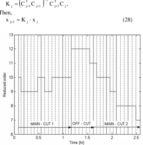
The reduced-orders are plotted with time as shown in Fig. 1. It is noted that by applying the model reduction the original full-states can be computed as a linear combination of the new reduced-states. In the off-cut operation, the highest reduced-orders are obtained because composition changes of the both components are significant. Afterwards the model-order decreases continuously in the production of toluene. Since the acetone amount in the column is completely exhausted and removed from the column, only seven new states are required for the last model.

Inferential composition estimation for a ternary batch column operated in an optimal operation has been further studied. For the EKF, the diagonal elements of both Σ0 and

Q are selected as 10-6. The diagonal elements of R for all the cases of measurements are defined as 100. For the proposed KF, a set of Q and R matrices are predefined, and scheduled according to the corresponding model equations. However, the matrix Σ0 is constant at 10

-5

.

It has been found that as instant distillate compositions remarkably change at time 5 minutes during the operation period, the estimators are activated. Both estimators have been tested with respect to the guess values of the initial-states. For the EKF estimator, the initial guess values are [0.4, 0.8, 0.9, 1, 1, 1, 1] and [0.4, 0.2, 0.1, 0, 0, 0, 0] for the first and second components respectively. For the linear estimator, the reduced-states are in the incremental changes then they are initialized by zero for the both productions. In addition, the initial guess of the distillate and reboiler compositions are chosen as [1, 0] and [0.3, 0.43] respectively.

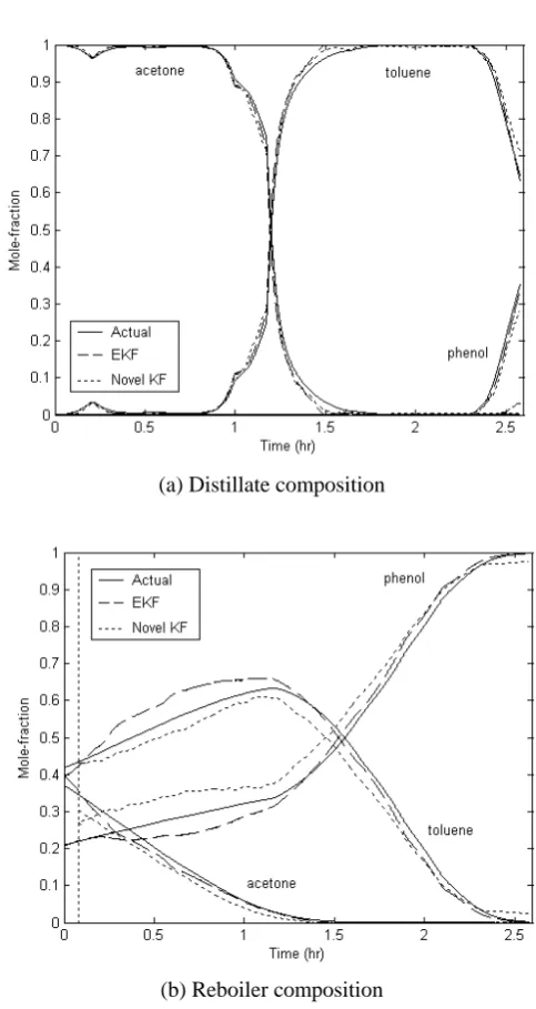
(a) Distillate composition

[image:5.595.309.551.77.532.2]

(b) Reboiler composition

Figure 2: Estimation profiles with noise ±1K

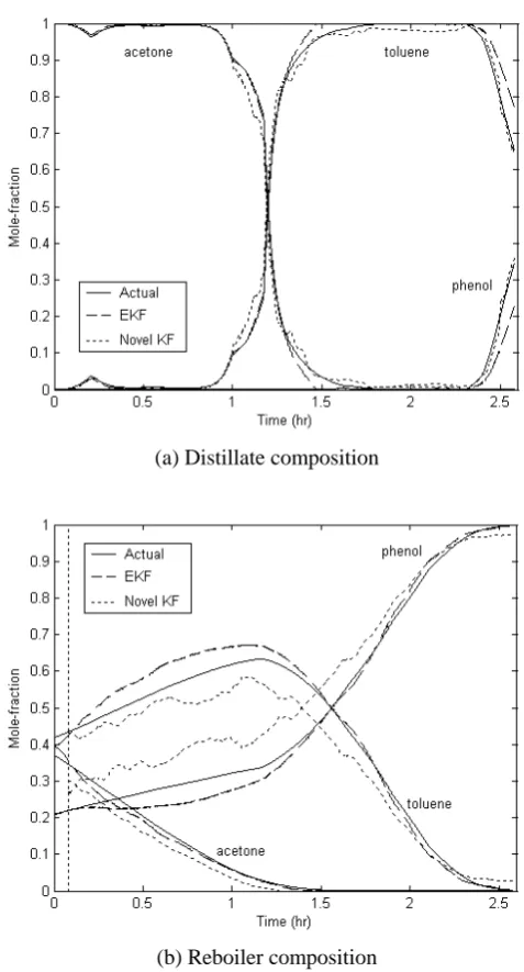
As available measurements usually involve statistical error therefore the sensors are corrupted by a Gaussian white noise with a zero mean and a certain standard deviation. As shown in Fig, 2, both nonlinear and linear estimators still give reasonable estimates of all products with the noise of the standard deviation of ±1Kelvin. The proposed estimator requires the computation effort only 56% of the one needed for the nonlinear estimator. However, it has been found that the linear estimator is rather sensitive to the high measurement noise ±3 Kelvin (Fig. 3).

VII. CONCLUSION

Vapor flow rate and holdups of tray and drum are constant for a whole batch operation, in which the values of the parameters are pre-determined in an optimal manner. For a linear KF, a set of reduced-order models is developed individually and employed sequentially to predict the whole batch behavior.

Simulation results have shown that both estimators give comparative estimation performances even in case of initial guessed conditions and measurement noise. However the state estimates obtained by the EKF will only converge to the actual values if accurate thermodynamic model is available. Although the proposed estimator performs rather sensitive to the effect of high measurement noise, however computation time is much lower than the ones required for the EKF. Moreover the knowledge of the thermodynamic is not required and the augmented states can be initialized easily by using zero values.

REFERENCES

[1] D. D. Yang, and K. S. Lee, “Monitoring of a distillation column using modified extended Kalman filter and a reduced order model” Comp. Chem. Eng., 21-S, 1997, pp. 565-570.

[2] J. Zhang, “Inferential feedback control of distillation composition based on PCR and PLS models” Proceedings of the American Control Conference, Arlington, VA June 2001, pp. 25-27.

[3] M. Kano, N. Showchaiya, S. Hasebe, I. Hashimoto, “Inferential control of distillation compositions: selection of model and control configuration” Cont. Eng. Prac., 11, 2003, pp. 927 – 933.

[4] E. Quintero-Marmol, W. L. Luyben, C. Georgakis, “Application of an Extend Luenberger Observer (ELO) to the control of multi-component batch distillation” Ind. Eng. Chem. Res., 30, 1991, pp.1870-1880.

[5] W. L. Luyben, Practical Distillation Control, Van Nostrand Reinhold, New York, 1992.

[6] M. Barolo, F. Berto, “Composition control in batch distillation: Binary and Multi-component mixtures” Ind. Eng. Chem. Res., 37, 1998, pp. 4689-4698.

[7] R. M. Oisiovici, S. L. Cruz, “State estimation of batch distillation columns using an extend Kalman filter” Chem. Eng. Sci., 55, 2000, pp. 4667-4680.

[8] C. Venkateswarlu, S. Avantika, “Optimal state estimation of multicomponent batch distillation” Chem. Eng. Sci., 56, 2001, pp. 5771 – 5786.

[9] C. Venkateswarlu, B. J. Kumar, “Composition estimation of multicomponent reactive batch distillation with optimal sensor configuration” Chem. Eng. Sci., 61, 2006, pp. 5560 – 5574.

[10] G. P. Distefano, “Mathematical models and numerical integration of multicomponent batch distillation equations” AIChE J., 14(1), 1968, pp. 190-199.

[11] I. M. Mujtaba, Batch Distillation: Design and Operation, Vol 3. Imperial College Press, UK, 2004.

[12] C. D. Holland, Fundamentals of multicomponent distillation, McGraw-Hill Book Company, USA, 1981.

[13] R. C. Reid, T. K. Sherwood, The properties of gases and liquids: 5th

edition, McGraw-Hill Book Company, New York, 2000.

[14] S. Skogestad, I. Postlethwaite, Multivariable feedback control: Analysis and Design, John Wiley and Sons, 1996.

(a) Distillate composition

[image:6.595.310.549.87.530.2]

(b) Reboiler composition