warwick.ac.uk/lib-publications
Original citation:
Irvine, Michael Alastair, Jackson, E. L., Kenyon, Emma J., Cook, Kevan J., Keeling, Matthew
James and Bull, J. C.. (2016) Fractal measures of spatial pattern as a heuristic for return rate
in vegetative systems. Royal Society Open Science , 3 (3). 150519.
Permanent WRAP URL:
http://wrap.warwick.ac.uk/79252
Copyright and reuse:
The Warwick Research Archive Portal (WRAP) makes this work of researchers of the
University of Warwick available open access under the following conditions.
This article is made available under the Creative Commons Attribution 4.0 International
license (CC BY 4.0) and may be reused according to the conditions of the license. For more
details see:
http://creativecommons.org/licenses/by/4.0/
A note on versions:
The version presented in WRAP is the published version, or, version of record, and may be
cited as it appears here.
rsos.royalsocietypublishing.org
Research
Cite this article:Irvine MA, Jackson EL,
Kenyon EJ, Cook KJ, Keeling MJ, Bull JC. 2016 Fractal measures of spatial pattern as a heuristic for return rate in vegetative systems.
R. Soc. open sci.3: 150519.
http://dx.doi.org/10.1098/rsos.150519
Received: 19 November 2015 Accepted: 2 March 2016
Subject Category:
Biology (whole organism)
Subject Areas:
ecology
Keywords:
return rate, fractal growth, self-organization, persistence, ecological indicators, Korcak exponent
Author for correspondence:
J. C. Bull
e-mail:[email protected]
Fractal measures of spatial
pattern as a heuristic for
return rate in vegetative
systems
M. A. Irvine
1
, E. L. Jackson
2
, E. J. Kenyon
3
, K. J. Cook
4
,
M. J. Keeling
5
and J. C. Bull
6
1Centre for Complexity Science, Zeeman Building, University of Warwick,
Coventry CV4 7AL, UK
2School of Medical and Applied Sciences, Central Queensland University,
North Rockhampton, Queensland, Australia
3School of Life Sciences, University of Sussex, Brighton, UK
4Natural England, Truro, UK
5Mathematics Institute and Department of Biological Sciences, University of Warwick,
Gibbet Hill Road, Coventry CV4 7AL, UK
6Department of Biosciences, University of Swansea, Swansea, UK
Measurement of population persistence is a long-standing problem in ecology; in particular, whether it is possible to gain insights into persistence without long time-series. Fractal measurements of spatial patterns, such as the Korcak exponent or boundary dimension, have been proposed as indicators of the persistence of underlying dynamics. Here we explore under what conditions a predictive relationship between fractal measures and persistence exists. We combine theoretical arguments with an aerial snapshot and time series from a long-term study of seagrass. For this form of vegetative growth, we find that the expected relationship between the Korcak exponent and persistence is evident at survey sites where the population return rate can be measured. This highlights a limitation of the use of power-law patch-size distributions and other indicators based on spatial snapshots. Moreover, our numeric simulations show that for a single species and a range of environmental conditions that the Korcak–persistence relationship provides a link between temporal dynamics and spatial pattern; however, this relationship is specific to demographic factors, so we cannot use this methodology to compare between species.
1. Introduction
The description and prediction of spatial patterns in nature has fascinated theoreticians and applied ecologists alike for
2
rsos
.ro
yalsociet
ypublishing
.or
g
R.
Soc
.open
sc
i.
3
:1
50519
...
many years. Initially, the study of seemingly intractable, complex patterns in time and space was predominantly a descriptive science [1]. However, in the latter years of the previous century, theoretical advancements demonstrated that complex spatio-temporal patterns could be generated as emergent properties resulting from simple rules [2]. This opened the door to understanding the mechanistic basis of many types of ecological pattern, including regular [3] and fractal/scale-free geometries [4]. However, the inverse problem of inferring biological mechanisms from observations and measurements on ecological systems remains a key challenge [5–8]. In part this is because, surprisingly, very similar spatial patterns can arise from a wide range of environmental and underlying endogenous processes [9–11]. In this study, we combine theoretical analysis of a simple but generally applicable, spatio-temporal simulation model with statistical modelling of independent spatial and spatio-temporal datasets from a well-studied ecosystem: a temperate seagrass monoculture. We explore the theoretical and empirical relationships between spatial and temporal measures of underlying dynamics, as well as providing some discussion of the potential, and limitations, of using spatial metrics in order to quantify ecological dynamics.
Broadly speaking, a spatio-temporal system (such as a spatial vegetative system) will typically have a high number of dimensions and attempting to match model and data by comparing the precise locations of individuals would quickly become intractable for all but trivial system sizes. This introduces the idea of using summary statistics to encapsulate the key information pertaining to the underlying dynamics of a given ecological growth process [12]. Traditionally, these techniques have taken the form of statistics derived from longitudinal measures of the total population size, ignoring spatial structure [13–15]. One important measure of resilience is the return rate or engineering resilience [16,17]. Given a stable ecosystem, this measures how long on average it takes before the system returns to the stable equilibrium point following a disturbance. The return rate quantifies this, and can be taken mathematically as the dominant eigenvalue of the dynamic system around the stable equilibrium value. However, often in order to gain accurate statistics many sequential observations need to be taken over extended periods of time. By contrast, spatial statistics derived from remote sensing techniques have a high number of degrees of freedom: they can be produced rapidly, can generate large amounts of data and therefore, in theory may lead to insights similar to those from more classical long-term studies [2,18,19].
The theory of fractals and scaling has numerous applications in ecology and is intimately linked with the ideas of spatial dynamics and inferring process from pattern. The original theory, proposed by Mandelbrot, was used to explain certain seemingly ubiquitous patterns in nature [20]. Since this time there has been much tantalizing speculation over using fractal theory to elucidate ecologically meaningful parameters from spatial patterns.
A major application of fractal theory in ecology is in the scaling of vegetation patch sizes. The distribution can be described by a power law in certain settings such as semi-arid ecosystems [21]. The distribution also tends to develop an increasing truncated tail as the system moves closer to a critical threshold due to increasing environmental pressure [22]. This implies that a spatial snapshot of a vegetation distribution can be used to determine if an ecosystem is close to a threshold that would lead to ecosystem collapse. The truncation of the power law may not universally be an indicator of ecosystem collapse, where the simpler measure of coverage may provide a stronger indicator [23]. Also, for diatoms in intertidal mudflats the opposite relationship was found, where the truncation of the power law disappeared under increased grazing pressure [24]. Until now, there has been little direct comparison between the properties of patch sizes for a single snapshot and the long-term trends (over several years) of a vegetation population.
Patch-size distributions may also often be viewed as pure power laws with no truncation term, characterized by a single exponent that determines the patchiness of the spatial pattern. The exponent of
a power-law patch-size distribution, also known as the Korcak exponent,Kis defined given a patch area
Aand the number of patches observed of that sizeNA, using the relationship
NA∼A−K.
3
rsos
.ro
yalsociet
ypublishing
.or
g
R.
Soc
.open
sc
i.
3
:1
50519
...
the cover between two species [31]. Mandelbrot [20], and subsequently Hastings [25] and Sugihara [32] proposed that there should be a linear relationship between the Korcak exponent and the underlying dynamics of the process.
However, although the Korcak exponent and other measures related to persistence can be related for particular processes, in general, there is no standard relationship and each measure is independent [33]. It, therefore, remains an open problem whether such fractal exponents are able to give any insight into the persistence of an ecosystem and where the limitations are.
In this paper, we explore when there is a relationship between the spatial and dynamic persistence of an ecosystem and under what scenarios we should expect this relationship to develop. In particular,
we use eelgrass (Zostera marina), a key marine species around sheltered coastlines, as motivation and a
source of high-quality ecological data. The eelgrass around the Isles of Scilly (located off the southwest tip
of Cornwall, UK: 49.9◦N 6.3◦W) has the key feature that its temporal dynamics can be assembled from
extensive surveys over the past 20 years [34], while its spatial distribution has been assessed from aerial photography [35]. From our understanding of eelgrass dynamics, we develop a simple probabilistic cellular automata (PCA) model of clonal growth of vegetation in the presence of an environmental gradient that limits reproduction; we compare and contrast the findings of this model with the data available for eelgrass.
2. Lattice-based simulation with environmental gradient
2.1. Model development
In order to understand the factors that determine when a relationship between spatial and dynamic persistence (in terms of rates of return to equilibrium density) occurs, we developed an explicit spatial model that includes both demographic and environmental factors. This allows the study of each of these factors separately in order to determine which contribute to the persistence relationship.
We develop a mechanistic model for the clonal growth of vegetation in the presence of an environmental gradient. This model is formulated to capture the known behaviour of eelgrass, but could be parametrized to match a range of ecosystems with a monoculture as the foundation species. The gradient can be used to determine the boundary between regions where the clonal species can colonize and persist, and regions where it is unable to do so due to restrictions in the environment (wave energy, sea depth, temperature, etc.) For example, eelgrass will only colonize coastal regions where sunlight, nutrients and soft-sediment are sufficient, hence an obvious environmental gradient that would determine eelgrass growth is sea depth [36,37].
We consider a single species of plant that can reproduce by local clonal growth; the plants also experience intra-specific competition (competition for nutrients, light, ground water, etc.) from the extended local environment which impacts on their reproductive potential. Plants are assumed to die at a constant rate. The model is formulated as a PCA [38,39], based upon similar assumptions to the kinetic equation modelling vegetative growth given in [40]. Reproduction due to clonal growth or seeding and
intra-specific competition are both governed by spatial kernels (kBandkC) that determine the strength
of each process at a given distance. The model is defined on a squareN×Nlattice, where each lattice
site can either be occupied (1 for short-hand) or unoccupied (0). For ease of explanation, we conceptually consider a plant to occupy a single site, although this is not necessary for any of the results. The four
key functions that determine the dynamics of this species are:λ(x), which captures the environmental
gradient and is purely a function of the locationx;kB(d), which captures the rate at which new plants
are produced (on unoccupied sites) at a distancedfrom the plant (a Gaussian function with varianceσ12);
kC(d), which measures the degree of competition felt from a plant at distanced(another Gaussian function
with varianceσ22), whilekdetermines the strength of this competition on reproduction.
Mathematically, this can be written as
Px(0→1)=λ(x)
⎛
⎝
i:occupied
kB(x−oi)
⎞ ⎠
⎛
⎝1−k
i:occupied
kC(x−oi)
⎞
⎠ (2.1a)
and
Px(1→0)=μ, (2.1b)
whereoi is the location of theith occupied site. The environmental componentλ(x) determines how
4
rsos
.ro
yalsociet
ypublishing
.or
g
R.
Soc
.open
sc
i.
3
:1
50519
...
components: an environmental gradient in a given direction and a site-specific noise term to reflect random perturbations:
λ(x)=γl.x+ξηx.
Hereξis the strength of noise parameter (ηxare independent Gaussian noise terms with mean zero and
variance one),γ gives the slope of the environmental gradient andlis a unit vector that specifies the
direction of the gradient.
2.2. Model analysis
Simulations were performed on a 100×100 grid for 6×10⁴time steps after the system has reached an
equilibrium state, where the density of occupied sites fluctuates around a mean value. The dynamic (k,μ),
spatial (σ1,σ2) and environmental (γ,ξ) parameters were varied between simulations and the Korcak
exponent and return rate were calculated for each simulation run.
The return rate for the simulation is taken to be the expected rate of change in density around the long-term equilibrium, providing an exact counterpoint to the values calculated from the time-series
data. For a given spatial pattern at timet, the exact probabilities for the births and deaths at each
site can be calculated, and a single stochastic realization of these gives the spatial pattern for the next time step. A general form of the return rate can thus be calculated by summing over the probability of all birth events minus the probability of all death events. The expected rate of change of density is
thereforeE[ρi]=
iPt,i(B)−Pt,i(D), where each site is indexed with i. Around the equilibrium point,
this equation is linearized such thatE[ρt]=a+bρt. The return rate is the gradient of this linear equation
b, which was calculated through linear regression. The system was initialized with the north border,
where the environmental gradient is at its maximum, fully occupied. This border was fixed in order to ensure stochastic fade-out did not occur. Simulations were run until the population reaches statistical equilibrium, this is assessed as equilibrating of the population density. Once it has reached statistical equilibrium, the density and expected change in density is recorded for a given number of generations
N. Linear regression is then performed on the dataset and the gradient of regression is taken to be the
return rate.
For a given spatial model distribution, the Korcak exponent is calculated as follows. The size of each continuous cluster of occupied sites is calculated, producing a distribution of patch sizes. A power-law (Pareto) distribution is fitted to this data, with scaling exponent and minimum patch size, using
a maximum-likelihood estimator approach. The minimum patch size is taken to be 1 pixel (0.2×0.2 m),
in order to compare the model-generated and field-generated data directly, and the scaling exponent was estimated via a standard maximum-likelihood method [41].
For the first investigation, dynamic and spatial parameters of the model (corresponding to eelgrass
behaviour) were fixed and the environmental parameters were varied (ξ and γ) between 0 and 1.
Assuming each grid cell corresponds to a 20×20 cm area, dynamic and spatial parameters can be set
that capture the known behaviour of eelgrass. The death probability was kept constant atμ=0.2, the
spatial growth and competition scales were kept constant atσ1=0.5, σ2=1; while both high (k=0.8)
and low (k=0.2) competition factors were investigated.
For the second investigation, the dynamic parameters (kandμ) were varied between 0 and 1 for fixed
environment and spatial parameters (σ1=0.5,σ2=1,γ=0.5,ξ=0.1).
3. Field survey and aerial photography of seagrass meadows
The results from the simulation study are directly compared with the spatial and temporal seagrass data. The aim is to find under what circumstances a relationship between the return rate and the Korcak exponent should exist and then determine if such a relationship can be observed in this real system.
3.1. Seagrass meadow locations
We monitored five seagrass (Z. marina) meadows around the Isles of Scilly, UK (figure 1andtable 1) from
1996 to 2014, using rigorous and consistent methodology [34,42,43].
3.2. Survey protocol
Seagrass was surveyed annually, during the first week of August, by placing 25 quadrats (0.25×0.25 m)
5
rsos
.ro
yalsociet
ypublishing
.or
g
R.
Soc
.open
sc
i.
3
:1
50519
...
0 <15 m depth
seagrass MHWS
5 m
0.5 1 2 3 4
km
N
W E
S
Figure 1.The five surveyed sites in The Isles of Scilly, UK. blt, Broad Ledges Tresco; la, Little Arthur; htb, Higher Town Bay; ogh, Old
Grimsby Harbour; wbl, West Broad Ledges. Both time-series data in the form of annual surveys and spatial data in the form of a single aerial survey were conducted (adapted from [35]).
Table 1.GPS positions and depths relative to chart datum for the five seagrass survey sites (‘+0.5’ indicates this site is exposed at low
water, all other sites are fully sub-tidal).
site latitude and longitude depth (m) Broad Ledges Tresco 49◦56.4N, 06◦19.6W 0.2
. . . .
Higher Town Bay 49◦57.2N, 06◦16.6W +0.5
. . . .
Little Arthur 49◦56.9N, 06◦15.9W 1.0
. . . .
Old Grimsby Harbour 49◦57.6N, 06◦19.8W 0.6
. . . .
West Broad Ledges 49◦57.5N, 06◦18.4W 0.6
. . . .
predetermined as random rectangular coordinates (x,y) translated into polar coordinates (distance,
bearing), radiating from a chosen focal point. Randomization of quadrat locations was renewed each year and the maximum distance was 30 m from the focal point, close to the centre of each meadow.
3.3. Statistical modelling
We developed a metapopulation dynamic model of seagrass habitat occupancy, based on the classic Levins model [44]. Suitable habitat is defined as either occupied or vacant. The proportion of habitat
patches for meadowi,Ni, is dependent on colonization and extinction rates, with dynamics described
by a logistic function. In discrete time, this function can follow the standard linearization, such that
yt,i=ai+biNt,i, whereyt,i=log(Ni,t+1/Ni,t) [45].
In order to calculate the return rate, we estimated habitat occupancy as the proportion of replicate
quadrats that were occupied by seagrass each year, t, at each of the five survey sites (i=1,. . ., 5). In
its linearized form, the metapopulation model can be fitted to spatially replicated seagrass data using
a generalized additive model (GAM) framework, regressing yonN, with airepresented by sitewise
6
rsos
.ro
yalsociet
ypublishing
.or
g
R.
Soc
.open
sc
i.
3
:1
50519
...
[46]. The GAM fitting process implements a generalized cross-validation algorithm to assess the optimal degree of nonlinearity. Additionally, we captured differences in within-site temporal variance, as well as between-site correlation, by incorporating a full variance–covariance matrix, estimated directly from the
data (see [47] for full details of the method). The regressed valuebiis then taken as the estimate for the
return rate at sitei[17,48].
All analysis was performed using R v. 3.1.2 (R Core Team 2014), with additional functions from the packages: ggmap, ggplot2 and mgcv.
4. Results
The spatial-dynamic persistence relationship was compared when either the environmental parameters or the demographic parameters were varied. These relationships were then compared with the seagrass ecosystem, where the dynamic persistence was measured from the annual longitudinal study and the spatial patchiness was measured from the aerial photographic survey described in the methods.
4.1. Simulations
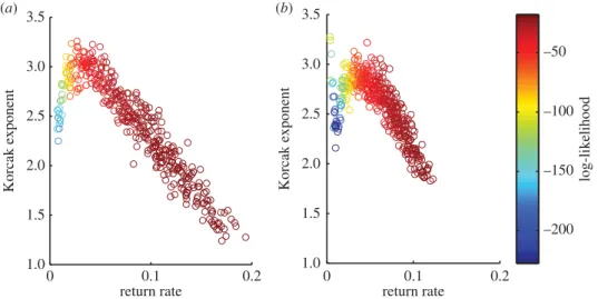
In the initial investigation, the dynamic and spatial parameters of the model were fixed and the environmental parameters were varied. The Korcak exponent correlates strongly with the return rate; there is also a high likelihood for each fitted power-law distribution, indicating a good fit of the exponent
(figure 2a,b). The gradient of the relationship was also found to vary depending on whether high
competition or low competition was present.
The environmental noise and gradient terms both have a large impact on the resulting return rate and
Korcak exponent of the system (figure 3a,b). A higher environmental gradient leads to a higher return
rate, with a decreased spatial patchiness (lower Korcak exponent). This effect is also more pronounced when the environmental noise term increases. The return rate and spatial patchiness is at its greatest value, where both the environmental gradient and noise are also at their greatest value.
In the second simulation experiment, the environmental parameters were fixed and the dynamic and spatial parameters were allowed to vary. The resulting Korcak exponent (figure 4) gives no relationship to the return rate. Although the spatial scaling does vary (between 2.8 and 3.7) there is no clear emergent
relationship and a linear regression analysis finds no significant trend (p>0.05).
The simulation analysis therefore indicates that a negative-linear relationship is found when sites are near equilibrium and when only environmental variables vary between sites.
4.2. Seagrass data analysis
Density dependence analysis was undertaken to quantify the return rate of seagrass metapopulations in equilibrium at each survey site. Here, return rate is the negative of the gradient of the density-dependent response around equilibrium [48]. Initially, the fitted variance–covariance matrix was assessed. Inclusion
of empirical between-site spatial correlations did improve model fit (Likelihood ratio=34.4, d.f.=10,
p<0.001). Generalized cross validation showed that a linear functional form, rather than smoothing
splines, was the best fit at all sites except Old Grimsby Harbour, making direct estimation of return rates
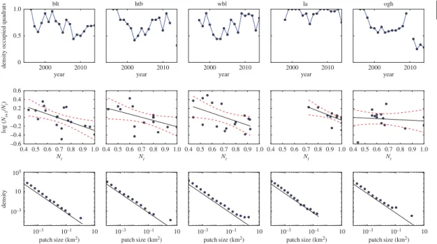
straightforward in all but that case (figure 5). Return rates are shown intable 2. At three survey sites,
Broad Ledges Tresco (blt), Higher Town Bay (htb) and West Broad Ledges (wbl), the null hypothesis of random walk dynamics was rejected in favour of density-dependent population regulation [13]. However, at Little Arthur (la) and Old Grimsby Harbour (ogh), statistically significant return rates could not be estimated (figure 5).
Seagrass persisted at all five survey sites throughout the length of the study (figure 5). There was
no evidence of temporal autocorrelation in the time series (Likelihood ratio=0.82,p=0.37). The only
site to show a significant linear trend (decline) was Old Grimsby Harbour (t=3.96,p<0.001). We found
the expected inverse relationship between the power-law exponent of the patch size distribution (the Korcak exponent) and the dynamic return rate, for survey sites that were confirmed as having stationary temporal dynamics (figure 6). However, two sites were excluded as they failed to meet this assumption: Old Grimsby Harbour is evidently in sharp decline (figure 5); and Little Arthur, while maintaining high
patch occupancy throughout the survey period, could not be confirmed as being stationary (figure 5and
7
rsos
.ro
yalsociet
ypublishing
.or
g
R.
Soc
.open
sc
i.
3
:1
50519
...
0 0.1 0.2 1.0
1.5 2.0 2.5 3.0 3.5
return rate
Korcak exponent
1.0
–50
–100
–150
–200 1.5
2.0 2.5 3.0 3.5
Korcak exponent
0 0.1 0.2 return rate
log-likelihood
(a) (b)
Figure 2.Relationship between return rate and Korcak dimension for high and low competition, where environmental parameters
were varied. Other parameters were kept constant atσ1=0.5,σ2=1 andμ=0.2. The log-likelihood indicates goodness of fit to the spatial data, where higher values indicate a better fit. (a) Korcak dimension (lowk) and (b) Korcak dimension (highk).
1.00
0.18 3.2
3.0 2.8 2.6 2.4 2.2 2.0 1.8 1.6 1.4 0.16
0.14 0.12 0.10 0.08 0.06 0.04 0.02 0.75
x
g
0.50
0.25
1.00
return rate
Korcak exponent
0.75 0.50 0.25
1.00
0.75
x
g
0.50
0.25
1.00 0.75 0.50 0.25 (b)
(a)
Figure 3.Resulting values of (a) return rate and (b) Korcak exponent for environmental noise (ξ) and environmental gradient (γ),
where competition (k) is low. Both environmental noise and gradient have a large impact on both the static and dynamic properties of the system. A sharper gradient increases the return rate and this effect is more pronounced for higher environmental noise. The gradient term also decreases the patchiness of the vegetation distribution (lower exponent), and this effect again increases for higher values of noise.
0.02 0.04 0.06 0.08 0.10 2.7
2.8 2.9 3.0 3.1 3.2 3.3 3.4 3.5 3.6 3.7
Korcak exponent
return rate
log-likelihood
−250 −200 −150 −100 −50
Figure 4.Varying the dynamic parameterskandμfor fixed spatial and environment parametersσ1=0.5,σ2=1,γ=0.5 and
8
rsos
.ro
yalsociet
ypublishing
.or
g
R.
Soc
.open
sc
i.
3
:1
50519
...
blt htb wbl la ogh
0.5
2000 2010 2000 2010 2000 2010 2000 2010 2000 2010
year year year year year
density occupied quadrats
log (
Nt+1
/
Nt
)
density
0
0.6 0.4 0.2 0 –0.2 –0.4 1.0
–0.6
0.4 0.5 0.6 0.7
Nt
0.8 0.9 1.0 0.4 0.5 0.6 0.7
Nt
0.8 0.9 1.0 0.4 0.5 0.6 0.7
Nt
0.8 0.9 1.0 0.4 0.5 0.6 0.7
Nt
0.8 0.9 1.0 0.4 0.5 0.6 0.7
Nt
0.8 0.9 1.0
105
10–3
10–3 10–1
patch size (km2)
10 10–3 10–1
patch size (km2)
10 10–3 10–1
patch size (km2)
10 10–3 10–1
patch size (km2)
10 10–3 10–1
patch size (km2)
10 10
Figure 5.Time-series and patch-size data from five survey sites around the Isles of Scilly, UK (blt, Broad Ledges Tresco; htb, Higher Town
Bay; wbl, West Broad Ledges; la, Little Arthur; ogh, Old Grimsby Harbour). The three sites used in the study are on the left, with the two excluded on the right.Top row: Data points represent proportions of occupied 25×25 cm quadrats for the years 1996–2014.Middle row: Transformed data, comparing density at yeartto log(Nt+1/Nt). Regression line for return rate shown in black with 95% confidence limit shown as a red dashed line.Bottom row: Patch-size distribution for five sites, with normalized frequency. A solid line with a scaling of 2 has been added for clarity.
Table 2.Estimated return rates and Korcak exponent for the five seagrass survey sites. Also given are the standard error (s.e.) of the
return rate fit along with thet-value and correspondingp-value and the 95% CIs for the Korcak exponent estimated through bootstrap re-sampling.
site return rate s.e. t-value (d.f.=50) p-value Korcak exponent 95% CI
blt 0.857 0.307 2.79 0.007 1.775 (1.773, 1.776)
. . . .
htb 0.718 0.296 2.33 0.023 1.869 (1.866, 1.869)
. . . .
la 0.943 0.618 1.52 0.134 1.761 (1.758, 1.762)
. . . .
ogh n.a. n.a. n.a. n.a. 1.811 (1.806, 1.813)
. . . .
wbl 0.930 0.294 3.04 0.004 1.740 (1.735, 1.740)
. . . .
5. Discussion
There has recently been increasing interest in finding generic spatial indicators of ecosystem pressure or collapse [22,49]; however, until now there has been little validation of these spatial indicators against long-term population data. We have demonstrated for a particular ecosystem under what circumstances there should be a connection between the dynamic persistence, defined using the return rate to population equilibrium, and the spatial persistence, defined using the Korcak exponent. The simulations derived from a model of a spatial dynamic vegetation system in the presence of demographic competition and an environmental gradient demonstrated that a strong relationship exists only when environmental parameters vary between sites. This relationship was then compared with a long-term seagrass study, where a similar relationship was found for the sites where the return rate could be measured.
9
rsos
.ro
yalsociet
ypublishing
.or
g
R.
Soc
.open
sc
i.
3
:1
50519
...
return rate
0.5 0.6 0.7 0.8 0.9 1.0 1.1 1.2 1.3
Korcak exponent
1.5 1.6 1.7 1.8 1.9 2.0 2.1
BLT HTB
LA
WBL
95% CI 85% CI
Figure 6.Korcak return rate relationship for surveyed vegetation. Empirical seagrass data for three sites surveyed is shown as labelled
points with±s.e. error bars for both return rate and Korcak exponent, where the Korcak exponent errors were found through bootstrap re-sampling [50]. Although Little Arthur (LA), did not have a statistically significant return rate, this has been plotted here for clarity. The diagonal solid band describes the inverse relationship reproduced by the PCA model over a range of environmental parameters. The overall simulation rate is set using known parameters of death and recruitment forZostera marina[51]. The other simulation parameters were set arbitrarily and hence show a qualitative as opposed to quantitative similarity with the data.
our knowledge, this is the first time a direct comparison has been possible between time-series and spatial snapshot data on the same natural system. The strategy of coupling rigorous modelling development with high-quality, long-term field study is a powerful approach for making generalizable inference based on biologically well-supported assumptions and observation. In particular, analysis of where the predicted relationship breaks down in nature, where the demographic parameters between locations are significantly different, provides useful motivation and insight for further theoretical exploration.
Using a PCA model, we predict a strong negative linear relationship between the Korcak exponent and the return rate over a wide range of parameters—in fact all parameters that generate return rates above 0.05 (figure 2). This reversal of the relationship can be observed when there is no environmental gradient present (figure 3). While variation in environmental parameters gave a strong Korcak–return rate relationship, this was not duplicated when the dynamic (species-specific) parameters were varied (figure 4). Instead a very low correlation relationship was found. These results highlight the practical usefulness and potential shortcomings of this method for discerning the return rate and hence persistence
of a species from its spatial pattern. The change in gradient due to high- and low-competition (k) values
also gives an indication of how comparisons of the Korcak exponent should be implemented (figure 2). If
endogenous parameters (k,σ1,σ2,μ) are fixed then a monotonic relationship is produced with a gradient
that is dependent on those endogenous parameters. This suggests that while in some settings the Korcak exponent does correlate with the return rate of the system and thus its persistence, this is not true in general. Other studies have recently highlighted similar results that generic indicators of a catastrophic shift may not hold generally across all settings [19,23,52].
10
rsos
.ro
yalsociet
ypublishing
.or
g
R.
Soc
.open
sc
i.
3
:1
50519
...
be system-dependent and further validation against empirical data is required before drawing robust conclusions from spatial snapshots alone [52].
In the event, only three out of five sites assessed showed the predicted relationship between spatial and temporal statistics. In both cases where the relationship between spatial and temporal dynamics fell down, it was due to being unable to reliably estimate a return rate from time-series analysis. At one site (Little Arthur), coverage by vegetation was very high for most of the time surveyed. Although population growth rate and density was reasonably described by a linear relationship (figure 5), this presented too little information about response to perturbation to derive a statistically significant return rate. The other site not following the predicted relationship was Old Grimsby Harbour, which is heavily disturbed by boat traffic and can be seen to be declining precipitously (figure 5). These cases point to limitations of classic time-series analysis. It would require further validation of the Korcak exponent approach to confidently use alongside time-series analysis.
Sugihara [32] proposed that dynamics could be inferred from complexity of shape. They illustrated this point, by using a fractional Brownian motion model where the Hurst exponent could be used to detect the persistence of the generating process. Other studies [53] have used this relationship to explore how measures of persistence can relate to dynamics; however, there has been no strong quantitative test of whether the spatial persistence of a landscape relates to the temporal persistence. Here we have tested the generality of this hypothesis by precisely defining dynamic persistence and then relating this to the shape of the resulting distribution. Overall, care must be taken when directly comparing spatial statistics to temporal ones. This general conclusion has also been recently highlighted in the context of comparing truncations in the patch-size distribution to the proximity to a dynamic threshold [22,23]. Universality of fractal growth processes leads to many spatial patterns that are similar in the sense that they share the same scaling relationship [54]. For a fractal measure to be applied in the context of estimating a return rate, we believe that a strong mechanistic understanding of the underlying growth mechanisms is required, which has similarly been found in a study of marine diatoms [24]. We have focused on mechanisms where growth is locally positively correlated with surrounding vegetation and negatively correlated on larger scales. However, there may also be other spatially correlated processes in a vegetative system that lead to changes in the scaling properties of the system such as grazing [22,23,55] or disease [56]. It would be interesting to discern the Korcak–persistence relationship where such other factors are present.
Data accessibility. The Isles of Scilly dataset including the patch sizes and occupancy for the five meadow sites can be
found at:http://dx.doi.org/10.5061/dryad.r95s8.
Authors’ contributions. M.A.I., M.J.K. and J.C.B. conceived the study. M.A.I. undertook the modelling, with support from
M.J.K. and J.C.B. E.L.J., E.J.K., K.J.C. and J.C.B. undertook the experimental work. M.A.I., M.J.K. and J.C.B. wrote the manuscript, with suggestions and comments from all authors.
Competing interests. The authors declare they have no competing interests.
Funding. The research in this article was in part funded by The University of Warwick’s EPSRC-funded Doctoral
Training Centre for Complexity Science.
References
1. Moffat AS. 1994 Theoretical ecology: winning its spurs in the real world.Science263, 1090–1092. (doi:10.1126/science.8108725)
2. Bascompte J, Solé RV. 1995 Rethinking complexity: modelling spatio-temporal dynamics in ecology. Trends Ecol. Evol.10, 361–366. ( doi:10.1016/S0169-5347(00)89134-X)
3. Rietkerk M, Van de Koppel J. 2008 Regular pattern formation in real ecosystems.Trends Ecol. Evol.23, 169–175. (doi:10.1016/j.tree.2007.10.013) 4. Pascual M, Guichard F. 2005 Criticality and
disturbance in spatial ecological systems.Trends Ecol. Evol.20, 88–95. (doi:10.1016/j.tree.2004.11. 012)
5. McIntire EJ, Fajardo A. 2009 Beyond description: the active and effective way to infer processes from spatial patterns.Ecology90, 46–56. (doi:10.1890/ 07-2096.1)
6. Borcard D, Legendre P, Avois-Jacquet C, Tuomisto H. 2004 Dissecting the spatial structure of ecological data at multiple scales.Ecology85, 1826–1832. (doi:10.1890/03-3111)
7. Jeltsch F, Moloney K, Milton SJ. 1999 Detecting process from snapshot pattern: lessons from tree spacing in the southern Kalahari.Oikos85, 451–466. (doi:10.2307/3546695)
8. Silvertown J, Wilson JB. 1994 Community structure in a desert perennial community.Ecology75, 409–417. (doi:10.2307/1939544)
9. Eppinga MB, de Ruiter PC, Wassen MJ, Rietkerk M. 2009 Nutrients and hydrology indicate the driving mechanisms of peatland surface patterning. Am. Nat.173, 803–818. (doi:10.1086/598487) 10. Liu QX, Weerman EJ, Herman PM, Olff H, van de
Koppel J. 2012 Alternative mechanisms alter the emergent properties of self-organization in mussel
beds.Proc. R. Soc. B279, 2744–2753. (doi:10.1098/rspb.2012.0157)
11. Liu QX, Doelman A, Rottschäfer V, de Jager M, Herman PM, Rietkerk M, van de Koppela J. 2013 Phase separation explains a new class of self-organized spatial patterns in ecological systems.Proc. Natl Acad. Sci. USA110, 11 905–11 910. (doi:10.1073/pnas.1222339110)
12. Dieckmann U, Law R. 2000 Relaxation projections and the method of moments. InThe geometry of ecological interactions: simplifying spatial complexity(eds U Dieckmann, R Law, JAJ Metz), pp. 412–455. Cambridge, UK: Cambridge University Press.
11
rsos
.ro
yalsociet
ypublishing
.or
g
R.
Soc
.open
sc
i.
3
:1
50519
...14. Ives A, Dennis B, Cottingham K, Carpenter S. 2003 Estimating community stability and ecological interactions from time-series data.Ecol. Monogr.73, 301–330. (doi:10.1890/0012-9615(2003)073[0301: ECSAEI]2.0.CO;2)
15. Berryman A, Turchin P. 2001 Identifying the density-dependent structure underlying ecological time series.Oikos92, 265–270. (doi:10.1034/j. 1600-0706.2001.920208.x)
16. Holling CS. 1996 Engineering resilience versus ecological resilience. InEngineering within ecological constraints(ed. P Schulze), pp. 31–44. Washington, DC: National Academy. 17. Sibly RM, Barker D, Denham MC, Hone J, Pagel M.
2005 On the regulation of populations of mammals, birds, fish, and insects.Science309, 607–610. (doi:10.1126/science.1110760)
18. Legendre P, Fortin MJ. 1989 Spatial pattern and ecological analysis.Vegetatio80, 107–138. (doi:10.1007/BF00048036)
19. Dakos V, Kéfi S, Rietkerk M, Van Nes EH, Scheffer M. 2011 Slowing down in spatially patterned ecosystems at the brink of collapse.Am. Nat.177, E153–E166. (doi:10.1086/659945)
20. Mandelbrot BB. 1983The fractal geometry of nature. New York, NY: Macmillan.
21. Scanlon TM, Caylor KK, Levin SA, Rodriguez-Iturbe I. 2007 Positive feedbacks promote power-law clustering of Kalahari vegetation.Nature449, 209–212. (doi:10.1038/nature06060)
22. Kéfi S, Rietkerk M, Alados CL, Pueyo Y, Papanastasis VP, ElAich A, de Ruiter PC. 2007 Spatial vegetation patterns and imminent desertification in Mediterranean arid ecosystems.Nature449, 213–217. (doi:10.1038/nature06111) 23. Maestre FT, Escudero A. 2009 Is the patch size
distribution of vegetation a suitable indicator of desertification processes?Ecology90, 1729–1735. (doi:10.1890/08-2096.1)
24. Weerman E, Van Belzen J, Rietkerk M, Temmerman S, Kéfi S, Herman P, Van de Koppel J. 2012 Changes in diatom patch-size distribution and degradation in a spatially self-organized intertidal mudflat ecosystem.Ecology93, 608–618. (doi:10.1890/11-0625.1)
25. Hastings HM, Sugihara G. 1993Fractals: a user’s guide for the natural sciences. Oxford, UK: Oxford University Press.
26. Pascual M, Roy M, Guichard F, Flierl G. 2002 Cluster size distributions: signatures of self–organization in spatial ecologies.Phil. Trans. R. Soc. Lond. B357, 657–666. (doi:10.1098/rstb.2001.0983) 27. Vicsek T, Family F. 1984 Dynamic scaling for
aggregation of clusters.Phys. Rev. Lett.52, 1669. (doi:10.1103/PhysRevLett.52.1669) 28. Irvine M, Bull J, Keeling M. 2015 Aggregation
dynamics explain vegetation patch-size
distributions.Theor. Popul. Biol.108, 70–74. (doi:10.1016/j.tpb.2015.12.001)
29. Xin Xp, Gao Q, Li Yy, Yang Z. 1999 Fractal analysis of grass patches under grazing and flood disturbance in an Alkaline grassland [J].Acta Bot. Sin.41, 307–313.
30. Imre AR, Cseh D, Neteler M, Rocchini D. 2011 Korcak dimension as a novel indicator of landscape fragmentation and re-forestation.Ecol. Indicators 11, 1134–1138. (doi:10.1016/j.ecolind.2010.12. 013)
31. Erlandsson J, McQuaid CD, Sköld M. 2011 Patchiness and co-existence of indigenous and invasive mussels at small spatial scales: the interaction of facilitation and competition.PLoS ONE6, e26958. (doi:10.1371/journal.pone. 0026958)
32. Sugihara G, May R. 1990 Applications of fractals in ecology.Trends Ecol. Evol.5, 79–86.
(doi:10.1016/0169-5347(90)90235-6) 33. Imre AR, Novotn`y J, Rocchini D. 2012 The
Korcak-exponent: a non-fractal descriptor for landscape patchiness.Ecol. Complexity12, 70–74. (doi:10.1016/j.ecocom.2012.10.001) 34. Bull JC, Kenyon EJ, Cook KJ. 2012 Wasting disease
regulates long-term population dynamics in a threatened seagrass.Oecologia169, 135–142. (doi:10.1007/s00442-011-2187-6)
35. Jackson EL, Higgs S, Allsop T, Cathray A, Evans J, Langmead O. 2011 Isles of Scilly seagrass mapping. Natural England NECR087.
36. Orth RJ, Moore KA. 1988 Distribution ofZostera marinaL. andRuppia maritimaL. sensu lato along depth gradients in the lower Chesapeake Bay, U.S.A. Aquat. Bot.32, 291–305. ( doi:10.1016/0304-3770(88)90122-2)
37. Krause-Jensen D, Pedersen MF, Jensen C. 2003 Regulation of eelgrass (Zostera marina) cover along depth gradients in Danish coastal waters.Estuaries 26, 866–877. (doi:10.1007/BF02803345) 38. Balzter H, Braun PW, Köhler W. 1998 Cellular
automata models for vegetation dynamics.Ecol. Model.107, 113–125. (doi:10.1016/S0304-3800 (97)00202-0)
39. Hogeweg P. 1988 Cellular automata as a paradigm for ecological modeling.Appl. Math. Comput.
27, 81–100. (doi:10.1016/0096-3003(88) 90100-2)
40. Lefever R, Lejeune O. 1997 On the origin of tiger bush.Bull. Math. Biol.59, 263–294. (doi:10.1007/ BF02462004)
41. Clauset A, Shalizi CR, Newman ME. 2009 Power-law distributions in empirical data.SIAM Rev.51, 661–703. (doi:10.1137/070710111)
42. Lobelle D, Kenyon EJ, Cook KJ, Bull JC. 2013 Local competition and metapopulation processes drive
long-term seagrass-epiphyte population dynamics. PLoS ONE8, e57072. (doi:10.1371/journal. pone.0057072)
43. Potouroglou M, Kenyon EJ, Gall A, Cook KJ, Bull JC. 2014 The roles of flowering, overwinter survival and sea surface temperature in the long-term population dynamics ofZostera marinaaround the Isles of Scilly, UK.Mar. Pollut. Bull.83, 500–507. (doi:10.1016/j.marpolbul.2014.03.035) 44. Levins R. 1969 Some demographic and genetic
consequences of environmental heterogeneity for biological control.Bull. Entomol. Soc. Am.15, 237–240. (doi:10.1093/besa/15.3.237) 45. Royama T. 1992Analytical population dynamics,
vol. 10. Berlin, Germany: Springer Science & Business Media.
46. Bjørnstad ON, Begon M, Stenseth NC, Falck W, Sait SM, Thompson DJ. 1998 Population dynamics of the Indian meal moth: demographic stochasticity and delayed regulatory mechanisms.J. Anim. Ecol.67, 110–126. (doi:10.1046/j.1365-2656.1998.00168.x) 47. Wood S. 2006Generalized additive models: an
introduction with R. Boca Raton, FL: CRC Press. 48. Sibly RM, Barker D, Hone J, Pagel M. 2007 On the
stability of populations of mammals, birds, fish and insects.Ecol. Lett.10, 970–976.
(doi:10.1111/j.1461-0248.2007.01092.x) 49. Kéfi S, Rietkerk M, Roy M, Franc A, De Ruiter PC,
Pascual M. 2011 Robust scaling in ecosystems and the meltdown of patch size distributions before extinction.Ecol. Lett.14, 29–35. (doi:10.1111/ j.1461-0248.2010.01553.x)
50. Efron B. 1981 Nonparametric estimates of standard error: the jackknife, the bootstrap and other methods.Biometrika68, 589–599. (doi:10.1093/biomet/68.3.589)
51. Larkum AW, Orth RJ, Duarte C. 2006Seagrasses: biology, ecology and conservation. Berlin, Germany: Springer.
52. Kéfi Set al.2014 Early warning signals of ecological transitions: methods for spatial patterns.PLoS ONE 9, e92097. (doi:10.1371/journal.pone.0092097) 53. Cunha A, Santos R, Gaspar A, Bairros M. 2005
Seagrass landscape-scale changes in response to disturbance created by the dynamics of barrier-islands: a case study from Ria Formosa (Southern Portugal).Estuar. Coast. Shelf Sci.64, 636–644. (doi:10.1016/j.ecss.2005.03.018) 54. Bunde A, Havlin S. 1991Fractals and disordered
systems. New York, NY: Springer. 55. Adler P, Raff D, Lauenroth W. 2001 The effect of
grazing on the spatial heterogeneity of vegetation. Oecologia128, 465–479. (doi:10.1007/s0044 20100737)