Analysis of the contour structural irregularity of skin lesions using wavelet decomposition

http://go.warwick.ac.uk/lib-publications

Original citation:

Ma, L. and Staunton, R. C. (2012). Analysis of the contour structural irregularity of skin lesions using wavelet decomposition. Pattern Recognition, 46(1)

Permanent WRAP url:

http://wrap.warwick.ac.uk/49978

Copyright and reuse:

The Warwick Research Archive Portal (WRAP) makes the work of researchers of the University of Warwick available open access under the following conditions. Copyright © and all moral rights to the version of the paper presented here belong to the individual author(s) and/or other copyright owners. To the extent reasonable and practicable the material made available in WRAP has been checked for eligibility before being made available.

Copies of full items can be used for personal research or study, educational, or not-for-profit purposes without prior permission or charge. Provided that the authors, title and full bibliographic details are credited, a hyperlink and/or URL is given for the original metadata page and the content is not changed in any way.

Publisher’s statement:

“NOTICE: this is the author’s version of a work that was accepted for publication in Pattern Recognition. Changes resulting from the publishing process, such as peer review, editing, corrections, structural formatting, and other quality control mechanisms may not be reflected in this document. Changes may have been made to this work since it was submitted for publication. A definitive version was subsequently published in Pattern Recognition, [VOL:46, ISSUE:1, January 2013)]

DOI:10.1016/j.patcog.2012.07.001” A note on versions:

The version presented here may differ from the published version or, version of record, if you wish to cite this item you are advised to consult the publisher’s version. Please see the ‘permanent WRAP url’ above for details on accessing the published version and note that access may require a subscription.

1

PRE-PRINT Accepted version, before formatting and proof reading. Final article

is in Pattern Recognition 46 (2013) 98–106

Analysis of the contour structural irregularity of skin lesions

using wavelet decomposition

Li Ma1 and Richard C. Staunton2 1

College of Life Information Science & Instrument Engineering, Hangzhou Dianzi University,

310018, China.

Email: [email protected] 2

School of Engineering, University of Warwick, Coventry CV4 7AL, U. K.

Email: [email protected]

Corresponding author: R.C. Staunton. Phone: +44 2476 523980, Fax: +44 2476 418922

Abstract

The boundary irregularity of skin lesions is of clinical significance for the early detection of

malignant melanomas and to distinguish them from other lesions such as benign moles. The

structural components of the contour are of particular importance. To extract the structure from

the contour, wavelet decomposition was used as these components tend to locate in the lower

frequency sub-bands. Lesion contours were modeled as signatures with scale normalization to

give position and frequency resolution invariance. Energy distributions among different wavelet

sub-bands were then analyzed to extract those with significant levels and differences to enable

maximum discrimination.

Based on the coefficients in the significant sub-bands, structural components from the original

contours were modeled, and a set of statistical and geometric irregularity descriptors researched

that were applied at each of the significant sub-bands. The effectiveness of the descriptors was

measured using the Hausdorff distance between sets of data from melanoma and mole contours.

The best descriptor outputs were input to a back projection neural network to construct a

combined classifier system. Experimental results showed that thirteen features from four

sub-bands produced the best discrimination between sets of melanomas and moles, and that a

small training set of nine melanomas and nine moles was optimum.

Keywords: melanoma detection, structural irregularity of contours, wavelet decomposition,

2

1. Introduction

Melanomas are malignant tumors comprised of epidermal or mucosal cells and have a high

possibility of lymphatic metastasis resulting in unfavorable prognosis. Early detection of

melanomas in clinics depends on a well-known ABCD rule to determine the benign or

malignant nature of skin lesions [1]. That is, Asymmetry of the lesion’s boundaries, Boundary

irregularity, Color distributions and lesion Diameters. Alternative classifications based on color

texture appearance has been researched recently [2, 3], and by employing a biopsy and electron

tomography, a classification from 3D cell images has been reported [4]. The technique of

dermoscopy used polarized light or oil coverage to make more of a lesion’s structure visible [5].

CAD systems have been researched to aide the clinician. These oftencomprise image

acquisition, artifact detection, lesion segmentation, feature extraction and lesion classification

stages [6].

In the previous decade, there have been many studies concerningthe boundary irregularity of

lesions using both geometric [7,8,9,10] and local fractal [11] measures. There are two types of

irregularities found on boundaries: textual and structural, these correspond to fine changes and

obvious convex and concave features respectively [7]. The structural irregularity has clinical

importance for melanoma diagnosis. The first task of boundary irregularity analysis is to

identify and extract the boundary as a 1D signal from the 2D image. The contours of skin

lesions can be considered as a mixture of structural and textural irregularity as can be seen by

following those in Fig.1. The benign mole is smooth with little variation on its contour, while

that of the melanoma contains many indents and protrusions in its structure, and has an obvious

visual roughness. However, for measurements of structural irregularity, multi-scale analysis of

skin lesion boundaries is an important technique for correctly isolating the structural from the

textural information. Wavelet transforms are useful multi-resolution analytical tools for

revealing object information at a defined scale or to select particular frequency bands of interest

[12]. A requirement for the design of structural irregularity descriptions is to explore ways of

extracting features not only from structural variations along the original contour, but also to

separate the scaled information in the significant sub-bands and thus with this extra information

to improve the accuracy of the diagnosis.

Previously T. K. Lee proposed an irregularity measure based on a deduced scale level using a

curvature model of multi-scaled boundaries [7]. However it involved heavy computation as the

proposed irregularity index was evaluated from a hierarchical structure with its roots as global

curve segments and leaves as local segments for each of the consecutive smoothed contours.

The Gaussian smoothing-scale increases on the original lesion contour indicated the evolution

of the curve’s indented and protruding segments.

The motivation for this study is to show that the filtered information in the sub-bands can be

used by structural irregularity descriptors to provide a good separation between melanomas and

3

followed by the selection of significant sub-bands can be an appropriate approach for the

evaluation of structural irregularity. The novelty of the proposed structural irregularity features

is:- (1) The extracted structural components of the contours are reconstructed by the summation

of the approximate wavelet coefficients at the selected maximum scale and only those detail

coefficients that are from structurally significant sub-bands; (2) Two classes of statistical and

geometric irregularity descriptors are defined and used. These were evaluated in each of the

significant sub-band to determine firstly that they were independent and did not correlate with

other features, and secondly their effectiveness in distinguishing between melanomas and moles

was measured. Features were discarded if they did not separate sets of moles and melanomas

sufficiently in order to maintain a compact feature space.

The steps in the procedure to reconstruct just the structural components of the contours are:-

Perform a 1D wavelet decomposition to produce a series of detailed contour signals for all the

lesion contours in the data set; Calculate energy measures for each of the detail, that is high

frequency, sub-bands; Perform a Hausdorff Distance (HD) [13,14] analysis based on energy

values in each sub-band to determine which detail coefficients are significant for distinguishing

the two sets; Select the significant sub-bands; Label the sub-bands with scales below these as

containing the textural component of the contour and rejected them from further consideration;

Sum the approximation coefficients and the remaining detail coefficients to generate the

connected structural component of the contour. This procedure approximately isolates the

structural portion of the original contour, and then the irregularity descriptors are used to refine

this and partition the lesions appropriately.

(a) (b)

Fig.1 Images of skin lesions (a) mole (b) melanoma

Section 2 describes the procedure to extract the structural components of the lesion contours

including the wavelet decomposition, the scale normalization necessary to process contours of

different length, and the selection of the significant sub-bands. Section 3 discusses the design of

the statistical and geometric descriptors of contour irregularity that are applied at multi-scales.

4

feature vector is compact. Section 5 provides the experimental results for the significant

structural component extraction and feature evaluation. A combined classifier using a back

projection neural network is described together with issues concerning training and the

evaluation of the structure of the feature vector. Finally Section 6 provides conclusions.

2. Extraction of the structural components of the skin lesion contours 2.1 Wavelet decomposition of a lesion contour

The contour of a skin lesion in an image is described by the points. C={x1,y1,x2,y2,…,xN,yN}. There are two ways of to represent this 2D data as a 1D signal: 1) The contour is split into two

1D sub-vectors Cx={x1,x2,…,xN} and Cy={y1,y2,…,yN}; or 2) The contour is modeled as a signature Cr={r1,r2,…,rN} where the radial distance from the geometric center,

2 ' 2 ' ) ( )

(x x y y

r_i = _i− + _i− , i=1,2,…n and (x',y') is the coordinate of the geometric center of

the closed contour. The signature representation was adopted in the paper as it provided the

advantage of position invariance.

2.1.1 Scale normalization

It was noted that many moles have a shorter contour for a given nominal area than do

melanomas. Together with size variability between the samples in the database, this can lead to

variations in estimated frequency and resolution in the frequency domain. Scale normalization is

required to enable a comparison between moles and melanomas in this domain. The proposed

normalization was modified from [15] to give radius:





















<

+









=

′

otherwise

N

n

i

r

T

i

r

N

n

i

r

r

i

)

(

)

(

-)

(

µ

₁

µ

₂

i=1,2,…,N (1)

Where i is an integer used to resample the contour points with a spacing distance of (n/N) and

the ceiling function

 

is used to produce an integer index to r. The values µ1 and µ2 are the averaged radial distances of all the melanomas and benign moles respectively in the data base.

Their inclusion provides a mean value platform on to which the lowest level approximation

coefficients will be superimposed. T is a threshold used to determine if a mole has a small value of r. If so, r is increased to reach a similar size to that of a melanoma. For melanomas and large

moles, the value of r is never increased.

r

_i

′

is the radial distance of the ith point of a contour

5

2.1.2 Wavelet decomposition

Wavelet decomposition is a powerful tool for multi-scale signal analysis. By using a pair of

low-pass and high-pass filters, an original signal is decomposed into approximation and detail

coefficients with the approximations feeding into the next level of decomposition, and thus

creating a decomposition tree [16]. The tree structure of such a 1D wavelet decomposition is

shown in fig 2.

Fig.2 Tree structure of wavelet decomposition

A 1D wavelet decomposition is performed on a contour signature Cr. The approximate and

detail coefficients at scale i are given by

A

i

=

{

a

₁i

,

a

i₂

,



a

i_M

}

and

D

i

=

{

d

₁i

,

d

₂i

,



d

_Mi

}

respectivelywhere M = N / 2i. As the scale increases, the approximate coefficients are further decomposed into low and high frequency components at the next higher scale. Generally the

textural components of a contour occupy the lower scale, higher frequency bands, with the

energy distributed evenly between bands to give a relatively small total energy within each.

However the structural components generally have a larger energy and occupy the lower

frequency bands. By using wavelet decomposition to level s, an original contour signature Cr is

transformed to a series of sub-band signals As,Ds,Ds−1,D1covering the whole signal

frequency space at [0,1/2s f_max],[1/2if_max,1/2i−1f_max],i=s,s−1,,2,1 and fmax is half the sampling frequency. This represents a concatenation of the frequency bands from the lowest

to the highest. The task is to identify at which decomposition levels the structural components of

a lesion contour can be extracted and which sub-bands in the frequency domain are significant

6

2.2 Sub-band descriptions of contour structural components

For a 1D contour signal, the FFT provides the magnitude and phase against frequency. The

weakness of the FFT is that the spectral profiles are unrelated to the position of an event in the

boundary and the resolution is fixed throughout the frequency band. On the other hand the

discrete wavelet transform (DWT) presents the capability of confining signal components to

dyadically increasing width frequency bands with different resolutions. The left two columns of

Fig.3 present mole, and the right two melanoma data. The plot in the first row of the first

column is the FFT spectrum of a mole where the zero frequency component has been translated

to the center. The plot on the right indicates the sub-band division in the frequency domain

when two levels of wavelet decomposition are implemented. A1, A2, D1, D2, refer to approximate and detail signals. The plots in the rows below show the signals in each band. Similarly the two

columns on the right are for a melanoma. Differences can be seen between the mole and the

melanoma signals in the D1 and D2 _{bands. We continue to describe the selection of the bands}

which enable the best discrimination between moles and melanomas.

Fig.3 Spectral and wavelet comparisons between a mole and a melanoma. Mole: (a) FFT, (b) A1,

A2, D1, D2 wavelet coefficient frequency map, (c) A1, (d) D1, (e) A2, (f) D2; Melanoma: (g) FFT, (h) A1, A2, D1, D2 wavelet coefficient frequency map, (i) A1, (j) D1, (k) A2, (l) D2;

2.2.1 Significant sub-band selection

To obtain justthe contour’s structural components, several lower frequency sub-bands need to

be identified from which to reconstruct that portion of the original contour using both

multi-scale approximate and detail coefficients. The evaluation of the significant sub-band range

was performed between each of the sample sets by HD distribution analysis at each level of

wavelet decomposition [17]. When analyzing the decomposition of a contour signal, the total

energy at any decomposition level indicates the significance of that sub-band frequency to the

7

2

) (

∑

=

i j i

j D

E j=1,2,…n (2)

2.2.2 Procedure for investigating significant sub-band selection

An algorithm was developed to identify those sub-bands which enabled the largest

discrimination between moles and melanomas. Given a set of p benign mole contours,

}

,

,

,

{

₁b ₂b b_p

b

₌

_x

_x

_

_x

Ω

where x_kb was the kth contour,and a set of q melanoma contours,

}

,

,

,

{

₁m ₂m _qm

m

₌

_x

_x

_

_x

Ω

where x_km was the kth contour.

Step1. For a preset maximum level of wavelet decomposition n, calculate the wavelet energy for

every contour xb_k and x_kmwithin each set Ωb and Ωm. First perform wavelet decomposition to

obtain the detail sub-band signals, Dn, Dn-1, … D1, for each lesion contour, and then calculate the

energy for either x_kbor x_kmin each band, E_lkb and E_lkm, where sub-band

l

=

1

,

2

,



,

n

using Eq.(2).

Step2. Form energy sets

E

b

=

{

E

_lb₁

，

E

_lb₂

,



,

E

_lpb

}

and

E

m

=

{

E

_lm₁

，

E

_lm₂

,



,

E

_lqm

}

from the

individual energies calculated for each transformed benign and melanoma contour at each

sub-band l=1,2,,n.

Step3. Compute the HDl value between energy sets of moles

E

band melanomas

E

m for

each band l,l=1,2,,n. This measures the discrimination between the two classes for each

sub-band.

Step4. Plot the distribution of

HD

l with respect to sub-band number l. The sub-bands with

the highest HD are considered as the most significant and used in the final classification.

Step5. The sub-bands with the higher HDs are considered as significant bands for use in

classification.

2.2.3 Extraction of the structural component of a lesion contour

Based on the theory of wavelet reconstruction, the structural component of a lesion contour is

8

threshold st so that:

t

s s

s s

s A D D D

C = + + −1++ (3)

1

2

1 _{D D}

D

C st st

t = − + − ++ (4)

Where Cs contains lower-frequency information and represents the structural component of the contour, and Ct contains higher-frequency information and represents the textural component. Choosing both s and stare difficult tasks, as a large s generates many narrow sub-bands close to zero frequency. Although these will contain structural information that will be relatively free of

textural irregularity, there is an extra cost in increased computational complexity. A small s can lead to structural contours contaminated with textural irregularity. The value of stchosen is crucial to obtain useful structural and textural contour information. The significant sub-band

selection process described in Section 2.2.2 was run on the test data and in practice the HD

distribution (Fig. 4) produced had a single peak that lead to the straightforward selection of a

single, general value for st as described in Section 5.1.

3. Descriptors of contour irregularity at multiple scales

Irregularity measures of object boundaries are key components for shape related classifications.

They are used after the contour structural components have been extracted. There are two

categories of irregularity descriptors, with one based on statistical measures, and the other on

geometry. The descriptors are only extracted at the previously determined significant levels

Ω ∈

j

j, , where Ω is a significant level set formed by the sub-band selection procedure of Section 2.2.2.

3.1 Statistical measures

Together with the mean and variance of the energy of Dj at each significant level [9], the following features related to contour irregularity were defined:-

1) Entropy of wavelet energy,

( )

_ij

N

i j i

j p p

w log

1

∑

=

−

= (5)

where p_ij =E_ij Ej is the energy probability of the ith component of Dj , Ejis the total energy

of the coefficients in band j as calculated by eqn (2),and E_ij = D_ij2. The energy entropy measures the magnitude of signal fluctuations.

2) Ultimate width. For any signalX =

{

x₁,x₂,...x_N

}

, the ultimate width is defined as µ

σ

× =2

9

Where µ and σ are the mean and variance of signal X. A large width indicates sharp variations.

3.2 Geometric based irregularity measures

At each significant level j, a supposed structural component Cj, s ≥ j ≥ st of a contour is reconstructed from the wavelet coefficients, Cj = A

s

+ Ds + Ds-1 + … + Dj. In addition to a simple variance measure [11], the other irregularity measures of the reconstructed contours are

evaluated as:-

Radial Deviation, 1 |( )|

1

∑

= − = N i i r r N

RD (7)

where r is the mean radius of the contour signature.

Contour Roughness [8],

=

∑

−

= +

N

i i i

r

r

N

Ro

1 1

|

|

1

(8) Irregularity Measure, ) ( ) ( s s j S Area S C Area

IM = ⊕ (9)

where Ss is reconstructed from the approximate data, A s

, at the significant level s, and ⊕ is the exclusive-or operator.

4. Feature selection

Feature selection was performed to remove some measures that were too similar to others and to

identify those that were most independent for inclusion in an efficient feature vector. Initially 25

features were identified from six irregularity descriptors at four scales plus IM at the threshold scale st. Then a correlation analysis followed by a performance based feature selection was performed as detailed below.

4.1 Correlation analysis

Correlation analysis is a popular tool for removing those redundant features that have a strong

relationship to others within a feature vector [18]. Given a feature vector

F

{

t

₁

,

t

₂

,



,

t

_n

}

and a

10

(

)(

)

(

) (

_∑

)

∑

∑

= = = − − − − = m p j pj m p i pi m p i pj i pi ij z t z t z t z t 1 2 1 2 1

ρ (10)

where zi is the mean value of feature ti in the sample set and tpi is the value of ti for the sample xp. The absolute value of ρij indicates the correlation between ti and tj, so a redundant feature will have a large ρij.

The following is the procedure for removing redundant features using correlation analysis:-

Step 1. Given an original feature vector F and a sample set S, Calculate a matrix of correlation

coefficients,

ρ

_ij

,

i

≠

j

,

1

≤

i

,

j

≤

n

using Eq.(10). ;

Step 2. Given a preset threshold T, split the pairs of features (ti,tj ), where (i ≠ j, 1 ≤ i, j ≤ n),into

two sets, where

F

₁

=

F

|

ρ

_ij

<

T

,

i

≠

j

,

1

≤

i

,

j

≤

n

is a set that does not contain redundant

features in F, and

F

₂

=

{

t

_p

,

p

∈

{

i

,

j

})

|

ρ

_ij

≥

T

}

is generated by choosing either feature of a

highly correlated pair. Selection can equally be random, or we kept the one that computed most

efficiently.

Step 3 The final feature set after removing redundant components is given by

F

′

=

F

₁

∪

F

₂.

4.2 Performance based feature selection

After removing the redundant features from the vector, those remaining are largely independent.

Further analysis is then performed to select the best features based on their discrimination

performance. To evaluate the discrimination, the contribution to the correct classification for

each feature is evaluated [7]. Given a sample set of skin lesions with manually labeled classes

w1 and w2, representing benign moles and malignant melanomas respectively, the probability

distributionsP

(

t_i|w₂

)

, and

P

(

t

_i

|

w

₁

)

are evaluated for each feature. Suppose the prior

probabilities p(w1) and p(w2) are equal, then the posterior probabilities p

(

w₁|t_i

)

and

(

w ti

)

p ₂| will be closely related to

p

(

t

_i

|

w

₁

)

and p

(

t_i|w₂

)

. The classification is perfectly

separable when any value of p

(

t |w₂

)

≠0 has the corresponding value of p

(

t |w₁

)

=0, and

is absolutely inseparable when p

(

t|w₂

) (

= pt|w₁

)

at any point [19].

However, medically, the probability of a benign mole p(w1) is larger than that of a melanoma

11

)

(

)

|

(

)

(

)

|

(

x

w

₁

p

w

₁

p

x

w

₂

p

w

₂

p

>

, then

x

∈

w

₁. Here this is simplified to be

)

|

(

)

|

(

x

w

₁

p

x

w

₂

p

>

using

p

(

w

₁

)

=

p

(

w

₂

)

. This proposed simplification is justified when

)

|

(

x

w

₁

p

is located to the left side of

p

(

x

|

w

₂

)

. This is true as the features, measuring contour

roughness, take smaller values in moles than that in melanomas. In addition, our rule has the

same averaged error probability as the Bayesian, because if

)

|

(

)

|

(

x

w

₁

p

x

w

₂

p

>

,

p

(

w

₁

)

>

p

(

w

₂

)

, then

)

(

)

|

(

)

(

)

|

(

)

(

)

|

(

x

w

₁

p

w

₁

p

x

w

₂

p

w

₁

p

x

w

₂

p

w

₂

p

>

>

⇒

p

(

x

|

w

₁

)

p

(

w

₁

)

>

p

(

x

|

w

₂

)

p

(

w

₂

)

Generally conditional probabilities of the feature ti for two classes will be overlapped. The degree of overlapping of the two probability distributions was used as a measure of

classification error for any single feature ti.

Suppose

F

′

=

{

t

₁

,

t

₂

,



,

t

_r

}

was the feature vector after redundancy removal. The steps used

for performance based feature selection were:-

Step 1: Conditional probability distributions. For each feature t_i ∈F′, calculate the

conditional probability distributions

p

(

t

_i

|

w

₁

)

and

p

(

t

_i

|

w

₂

)

for benign and malignant

lesions in the sample sets;

Step 2: Accumulated probabilities. Given a threshold T, find an appropriate value of k to

compute the accumulated probabilities P_bi =∑k_j=1pb_j≥Tand P_mi =∑N_j=k+1pm_j for each

feature t_i . Where

p

b_jand

p

m_j are the jth values of

p

(

t

_i

|

w

₁

)

and

p

(

t

_i

|

w

₂

)

.

Step 3: Feature verification. For each feature

t

_i

∈

F

′

(1≤i≤ p), If

P

_bi ≥ T and P_mi ≥ T,

the feature ti is verified with a classification error of less than 1-T, otherwise ti is discarded. Where T is a preset value that is chosen to be large enough to secure a sufficient classification

accuracy. The final feature set is then

F

*

=

{

t

₁*

,

t

₂*

,



,

t

_q*

}

, t_i*∈F′(1≤i≤q,q≤ p).

5. Experimental results

Three experiments were performed:- Significant wavelet sub-band selection; Reconstruction of

skin lesion contour from wavelet decompositions; And an evaluation of the proposed

multi-scale descriptors of contour irregularity using a combined classifier based on a back

projection neural network

12

They were downloaded from the Dermnet Skin Disease Image Atlas database at

http://www.dermnet.com/. The images were randomly selected from the database, after viewing

to remove some images that contained defocussed patches. Most images were of size 120x120

pixels, and if not, they were converted to this size by resampling. Each was converted from

color to gray level before processing. For the purpose of classification, a training set was formed

by randomly selecting 31 moles and 36 melanomas from the sample set, with the remaining

samples being used as test samples. The experiments were implemented using MATLAB 7.6.

5.1 Significant level selection and reconstruction of the structural component of a contour

Based on the procedure for significant sub-band selection described in Section 2.2.2, the

significant levels were identified using the training set and the ‘db3’wavelet. The maximum

level of decomposition was preset to 10.Then the HD between the averaged sub-band energies

of the wavelet detail coefficients for each class was measured at each level. The distribution is

shown in Fig.4 where it can be seen that levels 1 to 5 have a low flat distribution, levels 6 to 9

have a monotonically increasing HD, and that the HD at level 10 has decreased again.

The coefficients in levels D1 to D5 cover the higher frequencies where there are similar small textural variations for both moles and melanomas. The detail coefficients in D10 _{locate at the}

low frequencies where there is somebasic structure, but for computational efficiency it was

found to be better to use this when included in the approximation set A9. Therefore, as expected, with HDs up to 3.1, the middle-frequency bands represented by D6 to D9 have been shown to contain significant discrimination information, and these were selected as the significant levels.

Fig.4 HD distribution of wavelet detail signals v. level

It is simple to reconstruct the structural components of the contour after the significant levels in

the wavelet decomposition stack have been determined. Fig.5 shows the extracted contours of a

13

and e) are the corresponding contours reconstructed from A9 and D1 to D5. The approximation coefficient, A9 has been included to give the basic structure of the contour onto which the more complex textural part has been superimposed. Fig.5 c) and f) are reconstructed from A9 and D6

to D9(s = 9, st= 6), that is the boundaries representing the structural portion of the original lesion. With the textural information removed, these have the property of the highest

discrimination between different lesion classes. In the remainder of the paper these significant

sub-bands will be referred to as the structural sub-bands.

Fig.5 Contours after wavelet reconstruction. (a) Mole - original, (b) Mole - textural, (c) Mole – structural, (d) Melanoma – original, (e) Melanoma – textural, (f) Melanoma – structural. (Angle

in degrees and Radius in pixels, with inner dotted circle at 100 and solid circle at 200).

5.2 Results of feature selection

As described in Section 4, the original feature vector consisted of 25 irregularity features that

were formed from seven measures, six of which were applied at each of four significant

sub-bands. At the first stage of feature selection, correlation analysis, nine of these features were

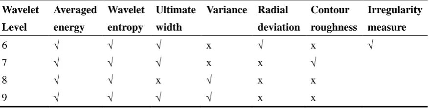
removed to decrease redundancy. Table 1 shows the retained (tick) and removed (cross) features.

The average energy, wavelet entropy and ultimate width were reliable features at most levels of

the significant sub-bands. The other independent features retained included the variance at the

two higher levels (8 and 9), the radial deviation at level 6, the contour roughness at level 7, and

14

Wavelet Level Averaged energy Wavelet entropy Ultimate width

Variance Radial deviation

Contour roughness

Irregularity measure

6 √ √ √ x √ x √

7 √ √ √ x x √

8 √ √ x √ x x

[image:15.595.78.517.91.202.2]

9 √ √ √ √ x x

Table 1. Results of feature selection after correlation analysis

After removal of the redundant features identified by the correlation analysis, selection was

taken further for the remaining 16 features by a classification performance analysis of each

feature. As discussed in Section 4.2, the cumulative probability distribution of each feature was

calculated for both the benign,

=

∑

= k i b i b

p

P

1

, and the melanomas,

=

∑

+ = N k i m i m

p

P

1

, in the sample

sets, where N was the largest observed value for that feature and k was a value satisfying

T p P k i b i b =

∑

≥

=1

. A threshold T = 0.75 was chosen experimentally that indicated correct

classification for every feature when applied to the benign samples in the training set. Then the

feature had to meet the requirement Pm > T to be retained within the overall feature vector. Fig.6 presents the results of the final feature selection.

Fig.6 Plot of accumulated probabilities:- (a) Pb ; (b) Pm, for each of the 16 features

[image:15.595.149.438.508.641.2]

15

further classification. It was noticed that some Pm values approached 1.0, signifying there was little overlap between the probability distributions of the benign and melanoma sets for these

features.

5.3 Combined classification results

The results of selections and tests on the individual features have been presented in Sections 5.1

and 5.2. In this section a Back Projection (BP) neural network is described that was used to

perform classification of skin lesions based on a combination of the 13 selected features. The

neural network had a structure of three layers:- input layer with 13 nodes; hidden layer with 3

nodes; and output with one node [20]. The training parameters were a preset training error of

0.01 and a maximum training number of 1000 iterations. As before, the main training set was

formed by randomly selecting 31 moles and 36 melanomas from the sample set, with the

remaining samples forming the testing set. A sub-set of the large training set was randomly

formed to produce an alternative small training set of 9 moles and 9 melanomas. To study the

discrimination ability of the proposed multi-scale based feature vector and to refine its operation,

some classification experiments were performed to compare firstly single-scale with multi-scale

features, and then multi-scale feature either before feature selection (25 features), or after (13

features). This was performed with both the small and large sized training sets to see which gave

the best results.

5.3.1 Before feature selection

Four experimental schemes were tried for training the BP network:- (1) Multi-scale, with all 25

features and the small training set; (2) Single scale, with 7 features at level 9 and the small training

set; (3) Multi-scale features and the large training set; and (4) Single scale features and the large

training set. After each training and processing of the test data, their corresponding Receiver

Operating Characteristic (ROC) plots were generated and are shown in Fig.7.

The input layer of the neural network has m values, where m is the number of features calculated

from each sample in the test data set. The output of the network produces a single real value between

0 and 1 to indicate which class the sample belongs to for each of the S samples in the test data set.

Overall the network produces an output vector with dimension S. Given a threshold value between 0

and 1, the output vector is converted to a binary vector with elements 0 and 1 indicating the class

estimations. Each sample in the set has previously been classified by a clinician and so the TP and

FP values for this threshold can be calculated. This process is repeated for a range of thresholds

between 0 and 1 and the resulting FP,TP pairs plotted as an ROC curve that spans from the bottom

left (1,0) to the top right corner (0,1).

The nearer the ROC trace is to the top left corner, the better the discrimination of a scheme

[21,22,23]. Fig.7 shows that the worst plot, is the single scale with a small training set, and the

16

small training set. This had a better classification power than the multi-scale scheme using the

large training set. The multi-scale features were always found to perform better than the single

scale features. In addition, the multi-scale features provided a way of improving the

discrimination when only a small sized training set was available.

Fig.7 ROC plots of the different training schemes before feature selection.

5.3.2 After feature selection

In this section the classification performances of the features selected by the different schemes

have been compared. Feature selection has only been reported for the multi-scale case as the

results of Section 5.3.1 have already confirmed multi-scale processing to be superior. The

following experiments were designed to compare the multi-scale features before and after

selection using both the large and small training sets. In order to reach a generality for the small

training set, an averaged ROC plot has been generated from 15 randomly selected possible

small training sets of 9 moles and 9 melanomas. In effect this was achieved by providing 15

parallel neural networks, averaging their real valued outputs, converting this to binary at each

threshold value from 0 to 1 and then plotting the TP, FP rates accumulated from all the test

samples on the ROC. The number of combination of all possible sets was too big to test

at

(

C₃₆9 ×C₃₁9

)

.

17

Results are with and without feature selection, and for large and small training image sets. From

Fig.8 the best classification performance is for 13 selected multi-scale features with a small

training set. It should be noted that this ROC plot has resulted from the averaged outputs of the

15 separately trained neural network classifiers using the test set. The next best is for the 13

selected multi-scale features with a large training set, followed by the 25 original multi-scale

features using the large training set, and finally the 25 original multi-scale features using the

small training set.

Fig.8 ROC plots for feature selection using multi-scale features

5.3.3 Design of parallel classifiers using small training sets

The results in Fig 8 have indicated that the averaged output of 15 neural classifiers using small

training sets can outperform a single classifier using a large training set.However a single

classifier using a small training set may or may not outperform that with a large training set. The

following experiments were performed to ascertain the optimum size of the training set.

For the many neural networks produced by training using randomly chosen small data sets, an

ROC plot from their averaged outputs was compiled after feeding the test data to each of them

18

plus moles were chosen at 3+3, 6+6, 9+9, 16+16, 23+23, 30+30, and tested together with the

large training set of 36+36. In the experiments 15 training sets were randomly selected for each

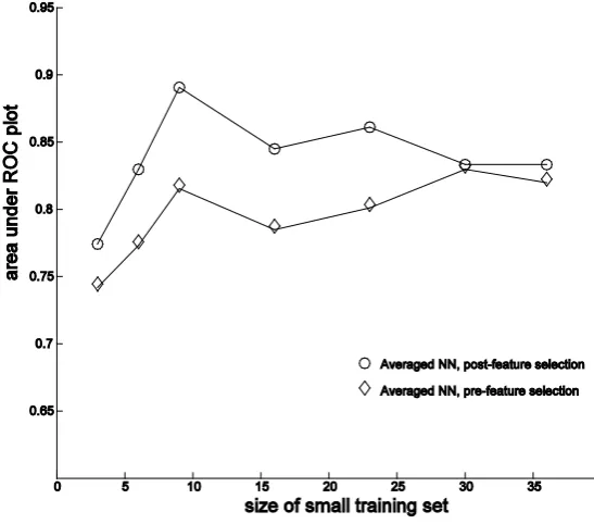
size from the full set of training data. Fig.9 presents the performance using the area under the

ROC plot against training set size for the pre- and post-selection schemes. The trace marked by

diamonds is for a ROC plot from the averaged outputs of the 15 classifiers before feature

selection whereas that marked by circles is post feature selection.

As indicated in Fig.9, the scheme using the averaged outputs of the 15 classifiers post-feature

selectionperforms best. It was noticed from the experiments that the averaged output value of all

networks, using a combination model of many parallel network classifiers, may overcome the

weakness of any single classifiers in the case of small training sets. The peak area of the ROC for

the averaged outputs of the neural network classifiers, post-feature selection was for a training

set of 9 melanomas plus 9 moles, indicating this to be the optimum size.

Fig.9 Performance against size of training set

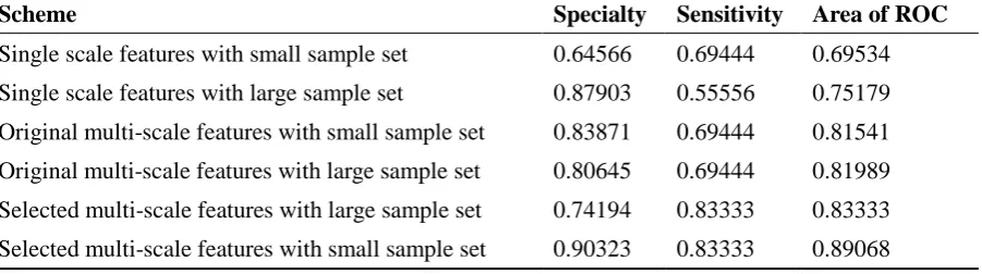
Table 2 lists the ROC performances for each of the two single scale and the four multi-scale

schemes tested. The performance is indicated by the measures of the sensitivity, specialty and

area covered by each ROC plot, where the paired values of sensitivity and specialty are the True

Positive Rate (TPR) and False Positive Rate (FPR) coordinates of the point on each ROC plot

closest to the top left corner [21,22,23]. With the lowest values, the single scale features with the

small training set have the worst results, and the multi-scale features after feature selection and

[image:19.595.127.401.312.553.2]

19

Scheme Specialty Sensitivity Area of ROC

Single scale features with small sample set 0.64566 0.69444 0.69534

Single scale features with large sample set 0.87903 0.55556 0.75179

Original multi-scale features with small sample set 0.83871 0.69444 0.81541

Original multi-scale features with large sample set 0.80645 0.69444 0.81989

Selected multi-scale features with large sample set 0.74194 0.83333 0.83333

[image:20.595.86.537.76.202.2]

Selected multi-scale features with small sample set 0.90323 0.83333 0.89068

Table 2. Comparison of classification performances

5.3.4 Discussion

In general, Fig.8 and Table 2 indicate that multi-scale features have better discrimination than

single scale features, and that, after feature selection, multi-scale schemes have better

performances than schemes without selection. The best ROC plot was for multi-scale selected

features using the small training set. It outperformed the corresponding scheme using the large

training set. There are two reasons for this in that each of the 13 selected multi-scale features

had a good individual performance when used for skin contour irregularity measurement and so

a small training set was probably sufficient. Secondly the performance of a neural network with

a BP training algorithm can be degraded by using a large training set that may cause a solution

to become stuck in a local minimum [24].

6 Conclusions

A method that examines the structural content of the contour of skin lesion images has been

proposed that determines if the lesion is a melanoma or a benign mole. The contour contained

both structural and textural information, but it was demonstrated that the structural information

was most important in the determination.

The 1D contour signal was filtered into sub-bands using the discrete wavelet transform (DWT)

down to level 9. The structural information was found to lie mostly at the lower frequencies, in

the detail levels from 6 to 9 plus the approximation at level 9. These were denoted as significant

levels, and the information within them was shown to provide the best classification separation

between sets of melanomas and moles. The DWT was found to enable efficient processing of

the signals.

A number of statistical and geometric feature descriptors of contour irregularity were developed.

These were computed in each of the significant sub-bands. To enable an efficient system, these

features were selected using a two stage process. Firstly correlation analysis was used to remove

redundant features, and secondly the performance of each feature in separating sets of

20

A classifier using a combination of features was designed using a back-projection neural

network. The system was optimized to obtain the maximum true positive rate and minimum

false positive rate for separation. Issues of training were explored, and a small, randomly chosen,

sub-set of 9 melanoma and 9 mole images found to provide the best results. Of the seven

available features, six were applied in four significant sub-bands and one in a single sub-band,

forming twenty five measurements in total. As described above these had been ranked in order

of effectiveness, and it was found the best combined classifier resulted when just the best

thirteen measures were used.

Acknowledgement:

This work is supported by National Scientific foundation of China (60775016).

References

[1] C. Grana, G. Pellacani, R. Cucchiara, S. Seidennari. A new algorithm for border description

of polarized light surface microscopic images of pigmented skin lesions, IEEE Transactions on

Medical Imaging 22 (8) (2003) 959-964.

[2] C. Serrano, B. Acha, Pattern analysis of dermoscopic images based on Markov random

fields, Pattern Recognition 42 (6) (2009) 1052-1057.

[3] A. Chiem, A. Al-Jumaily, R. N. Khushaba, A Novel Hybrid System for Skin Lesion

Detection, in: Proceedings of the 3rd International Conference on Intelligent Sensors, Sensor Networks and Information, ISSNIP, Melbourne, Australia, 2007, pp. 567-572.

[4] R. Narasimha, H. Ouyang, A. Gray, S. W. McLaughlin, S. Subramaniam, Automatic joint

classification and segmentation of whole cell 3D images, Pattern Recognition, 42 (6) (2009)

1067-1079.

[5] M. E. Vestergaard, P. Macaskill, P. E. Holt, S. W. Menzies, Dermoscopy compared with naked

eye examination for the diagnosis of primary melanoma: a meta-analysis of studies performed

in a clinical setting, British Journal of Dermatology 159 (3) (2008) 669-676.

[6] P. Wighton, T. K. Lee, H. Lui, D. I. McLean, M. S. Atkins, Generalizing common tasks in

automated skin lesion diagnosis, IEEE Transactions on Information Technology in Biomedicine

15 (4) (2011) 622-629.

[7] T. K. Lee, D. I. McLean, M. S. Atkins, Irregularity Index: A new border irregularity

measure for cutaneous melanocytic lesions, Medical Image Analysis 7 (1) (2003) 47-64.

[8] S. V. Patwardhan, A. P. Dhawan, P. A. Relue, Classification of melanoma using tree

structured wavelet transforms, Computer Methods and Programs in Biomedicine 72 (3) (2003)

223 – 239.

[9] K. M. Clawson, P. Morrow, B. Scotney, J. McKenner, O. Dolan, Analysis of pigmented skin

21

2009, pp. 18-23.

[10] X. Yuan, N. Situ, G. Zouridakis, A narrow band graph partitioning method for skin lesion

segmentation, Pattern Recognition 42 (6) (2009) 1017-1028.

[11] Li Ma, W. Xu, L. Zhu, Description of Boundary Irregularity On Multi-Scale Local FD for

Melanomas, in: Proceedings of the 3rd International Conference on Bioinformatics and Biomedical Engineering, Beijing, China, 2009, pp. 1-4.

[12] Y. C. Liao, K. C. Hung, C. T. Ku, C. F. Tsai, S. M. Guo, Wavelet octave energy for breast

tumor classification on sonography : A new shape feature, in: Proceedings of the IEEE

International Conference on Networking, Sensing and Control, Okayama, Japan, 2009, pp.

388-392

[13] D. P. Huttenlocher, G. A. Klanderman, W. J. Rucklidge, Comparing Images using the Hausdorff

Distance, IEEE Transactions on Pattern Analysis and Machine Intelligence 15 (9) (1993) 850-863.

[14] E. Yoruk, E. Konukoglu, B. Sankur, J. Darbon, Shape-based hand recognition, IEEE

Transactions on Image Processing 15 (7) (2006) 1803-1815.

[15] L. Yang, C. Y. Suen, T. D. Bui, P. Zhang, Discrimination of similar handwritten numerals

based on invariant curvature features, Pattern Recognition 38 (7) (2005) 947-963.

[16] G. Strang, T. Nguyen, Wavelets and Filter Banks, Wellesley-Cambridge Press, MA, USA,

1997.

[17] K. H. Lin, B. Guo, K. M. Lam, W. C. Siu, Human face recognition using a spatially

weighted modified hausdorff distance, in Proceedings of the International Symposium on

Intelligent Multimedia, Video and Speech Processing, Hong Kong, China, 2001, pp. 477-480.

[18] Y. Li, Z. F. Wu, J. M. Lui, Y. Y. Tang, Efficient feature selection for high-dimensional data

using two-level filter, in: Proceedings of the International Conference on Machine Learning and

Cyberntics, Shanghai, China, 2004, volume 3, pp. 1711-1716.

[19] D. T. Lin, C. R. Yan, W. T. Chen, Autonomous detection of pulmonary nodules on CT

images with a neural network-based fuzzy system Computerized Medical Imaging and Graphics

29 (6) (2005) 447-458.

[20] R. T. J. Bostock, E. Claridge, A. J. Harget, P. N. Hall, Towards a neural Network Based

System for Skin Cancer Diagnosis, in: Proceedings of the Third International Conference on

Artificial Neural Networks, Brighton, UK, 1993, pp. 215-219.

[21] T. Fawcett, ROC Graphs: Notes and practical considerations for researchers,

home.comcast.net/~tom.fawcett/public_html/papers/ROC101.pdf , HP Laboratories, Palo Alto, CA, USA, 2004

[22] T. Fawcett, An introduction to ROC analysis”, Pattern Recognition Letters 27 (8) (2006)

861-874.

[23] T. Fawcett, P. A. Flach, A response to Webb and Ting's On the application of ROC analysis

to predict classification performance under varying class distributions, Machine Learning 58 (1)

22

[24] W. Jin, Z. J. Li, L. S. Wei, H. Zhen, The improvements of BP neural network learning

algorithm, in: Proceedings of the 5th International Conference on Signal Processing, volume 3, Beijing, China, 2000, pp. 1647-1649.

About the Author ─ Li Ma received the B. S. and PhD degrees in Electrical Engineering from

Central South University, P. R. China, in 1976 and 1998 respectively. She is currently a

professor at the College of Life Information Science & Instrument Engineering, Hangzhou

Dianzi University, P. R. China. She has been an academic visitor to the College of Cardiff,

University of Wales, U.K. during 1993-1994, and a senior visiting fellow at the University of

Warwick in 2003. Her research interests include industrial and medical image processing, video

based monitoring systems, and pattern recognition.

About the Author─ Richard Staunton received the B.Sc. (honours) degree in electronic

engineering from the City University, UK, in 1973, and the Ph.D. degree in engineering from

the University of Warwick, UK, in 1992. He is currently an Associate Professor in the School of

Engineering at The University of Warwick, UK. From 1973 to 1977 he worked for the

aerospace industry and from 1977 to 1986 for the UK National Health Service, where he

engaged in research and development of medical image processing systems. His current

research interests include depth from defocus, industrial image processing, hexagonal sampling