Analysis of an energy based atomistic/continuum approximation of a vacancy in the 2D triangular lattice

http://wrap.warwick.ac.uk/

Original citation:

Ortner, Christoph and Shapeev, A. V.. (2013) Analysis of an energy-based

atomistic/continuum approximation of a vacancy in the 2D triangular lattice. Mathematics

of Computation, Volume 82 (Number 284). pp. 2191-2236.

Permanent WRAP url:

http://wrap.warwick.ac.uk/60455

Copyright and reuse:

The Warwick Research Archive Portal (WRAP) makes this work of researchers of the

University of Warwick available open access under the following conditions. Copyright ©

and all moral rights to the version of the paper presented here belong to the individual

author(s) and/or other copyright owners. To the extent reasonable and practicable the

material made available in WRAP has been checked for eligibility before being made

available.

Copies of full items can be used for personal research or study, educational, or

not-for-profit purposes without prior permission or charge. Provided that the authors, title and

full bibliographic details are credited, a hyperlink and/or URL is given for the original

metadata page and the content is not changed in any way.

Publisher’s statement:

© First published in Mathematics of Computation in Volume 82 (Number 284). pp.

2191-2236. published by the American Mathematical Society

http://dx.doi.org/10.1090/S0025-5718-2013-02687-7

A note on versions:

The version presented in WRAP is the published version or, version of record, and may

be cited as it appears here.

Volume 00, Number 0, Pages 000–000 S 0025-5718(XX)0000-0

ANALYSIS OF AN ENERGY-BASED ATOMISTIC/CONTINUUM APPROXIMATION OF A VACANCY IN THE 2D TRIANGULAR

LATTICE

C. ORTNER AND A. V. SHAPEEV

Abstract. We present ana priorierror analysis of a practical energy based atomistic/continuum coupling method (A. V. Shapeev, Multiscale Model. Simul., 9(3):905–932, 2011) in two dimensions, for finite-range pair-potential interac-tions, in the presence of vacancy defects.

We establish first-order consistency and stability of the method, from which we obtaina priorierror estimates in the H1_{-norm and the energy in terms of}

the mesh size and the “smoothness” of the atomistic solution in the continuum region. From these error estimates we obtain heuristics for an optimal choice of the atomistic region and the finite element mesh, as well as convergence rates in terms of the number of degrees of freedom. Our analytical predictions are supported by extensive numerical tests.

1. Introduction

The purpose of this work is a rigorous study of a new computational multiscale method coupling an atomistic description of a defect to a continuum model of the elastic far field.

The accurate computational modelling of crystal defects requires an atomistic description of the defect core, as well as an accurate resolution of the elastic far field. Atomistic-to-continuum coupling methods (a/c methods) have been proposed to combine the accuracy of atomistic modelling with the efficiency of continuum mechanics (see [14, 21, 31, 32, 34] for selected references, and [19] for a recent overview).

The construction of accurateenergy-baseda/c methods has been proven partic-ularly challenging, due to the so-called “ghost-forces” at the interface between the atomistic and continuum regions. This issue has been discussed at great length in [31, 4, 7, 20], and several interface corrections have been proposed to either remove or reduce the ghost forces [32, 7, 13, 34, 30, 12]. In general, the ghost-force removal problem remains unsolved.

A growing body of literature exists on the rigorous analysis of a/c methods (we refer to [30, 22, 18] for recent overviews), which has been largely restricted to one-dimensional model problems. We are currently aware of only two exceptions: (1) In

Received by the editor March 7, 2012.

2000Mathematics Subject Classification. 65N12, 65N15, 70C20.

Key words and phrases. atomistic models, atomistic-to-continuum coupling, coarse graining. This work was supported by the EPSRC Critical Mass Programme “New Frontiers in the Math-ematics of Solids” (OxMoS), by the EPSRC grant “Analysis of atomistic-to-continuum coupling methods”, and by the ANMC Chair at EPFL (Prof. Assyr Abdulle).

c

XXXX American Mathematical Society

[22] it is shown that, in 2D, any a/c method that has no ghost forces is automatically first-order consistent. This work provides a general consistency analysis, but does not address stability of a/c methods. (2) In [17], a force-based a/c method with an overlap region is analyzed, in particular providing sharp stability estimates. How-ever, the method proposed in [17] is not practical since it requires a prohibitively wide overlap region; moreover, the analytic methods employed cannot accommo-date defects, or coarse-graining of the continuum region. Some of these challenges have been overcome in [16], where it is shown that a fairly narrow blending width is sufficient to ensure stability of the method, however, a complete analysis of a practical variant of force-based blending remains open.

In the present work, we give an a priori error analysis of a practical energy-based a/c method proposed by Shapeev [30]. The formulation of the method and its analysis are restricted to pair interactions in two dimensions, with periodic boundary conditions.

For the case of a vacancy defect our analysis requires an assumption on the magnitude of the deformation field generated by the defect, but is otherwise fully rigorous. For more general “vacancy sets”, our consistency analysis remains fully rigorous, however, our stability analysis relies on a so-called vacancy stability index, which we estimate numerically (we give an analytical estimate for the single vacancy case).

Finally, we remark that the goal of a/c methods is to simulate far more complex situations than we can treat rigorously; we employ the example of a vacancy defect as the simplest non-trivial model problem.

1.1. Outline. In§2 we formulate an atomistic model for the 2D triangular lattice, with periodic boundary conditions, and two-body interactions. We also introduce a convenient notation for bonds.

In §3, we formulate the a/c method studied in this paper: the ECC method introduced in [30], but with periodic boundary conditions. This section contains all necessary results and notation required for an implementation of the a/c method, as well as a brief sketch of the proof of thea priorierror estimate in order to motivate the subsequent analysis.

In §4 we collect auxiliary results, which are largely technical results for finite element spaces. We also introduce a new measure of “smoothness” of discrete functions.

In§5 we prove consistency error estimates in discrete variants of the W−1,p-norm,

p∈[1,∞]. Our estimates are stronger and require fewer technical assumptions than the general result given in [22].

In§6 we develop the stability analysis. We introduce a “vacancy stability index”, which reduces the stability of a lattice with vacancies to stability of a lattice without defects. We provide numerical examples and one analytical estimation of stability indices.

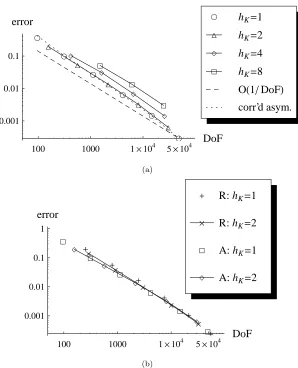
Finally, in§8, we present extensive numerical examples to confirm our analytical results, and to provide further discussions of points where our rigorous analysis is not sharp.

1.2. Notation. Fors, t∈R, we writes∧t:= min{s, t}. The`p_{-norms in}

Rk are denoted by| · |pand| · |:=| · |2. We do not normally

dis-tinguish between row and column vectors, but instead define three vector products: ifa, b∈Rk, thena·b:=Pkj=1ajbj, anda⊗b:= (aibj)

k

i,j=1, whereidenotes the row

index andjthe column index. Ifa, b∈_R2_{, then we also definea×b:=a1b2−a2b1.}

Matrices are usually denoted by sans serif symbols,A,B,F,G, and so forth. The set of k×k matrices with positive determinant is denoted by _Rk×k₊ . The set of rotations ofR2is denoted by SO(2). Throughout we will denote a rotation through angle π/2 by Q4 and a rotation through angle π/3 by Q6. If G ∈ Rk×k, then

kGk denotes its `2-operator norm, and|G|p the`p(Rk×k)-norm. In particular, |G| is the Frobenius norm, with the associated inner product F : G. The symmetric component of a matrixG∈Rk×k is denoted byGsym:=12(G+G

>_).

If A ⊂Rk is (Lebesgue-)measurable, then|A| denotes its measure. If A⊂R2 has Hausdorff dimension one, then we will denote its length by length(A). Volume integrals are denoted by dV, while surface (1D) integrals are denoted by ds. For bonds, which are specific one-dimensional objects, it will be convenient to introduce a slightly different notation (see§2.2 and§3.2).

The interior and closure of a setA⊂Rkare denoted, respectively, by int(A) and clos(A). IfA⊂R2is understood as a one-dimensional object, then we will also use int(A) to denote its relative interior, but will normally specify this explicitly.

The Lebesgue normsk · kLp_(A)for one- or two-dimensional measurable setsAare

defined in the usual way for scalar functions. If w: A →Rk is measurable, then

kwkLp_(A) :=k|w|2kLp_(A). Ifw is differentiable at a point x, then ∇w(x) denotes

its Jacobi matrix. The symbol D is reserved for finite differences, and will be introduced in§2.2.

2. _{The Atomistic Model}

2.1. The triangular lattice with vacancy defects. The 2D triangular lattice is the set

L#:=A6Z2, where A6:=a1,a2:=

_{1 1/2}

0 √3/2

,

whereai,i= 1,2, are called thelattice vectors. We furthermore seta3= (−12, √

3 2 )

>

andai+3=−aifori∈Z, so that the set ofnearest-neighbour directionsis given by

Lnn:=

aj:j= 1, . . . ,6 =

Qj−1₆ a1:j= 1, . . . ,6 ,

where Q6 ∈ SO(2) denotes the rotation through π/3. Finally, we denote the set

of all lattice directionsby _L∗:=L#\ {0}. The hexagonal symmetry ofL# yields the following result, which decomposes the triangular lattice into lattice vectors of equal distance.

Lemma 2.1. There exists a sequence (rn)∞_n=1 ⊂ L∗ such that `n := |rn| is monotonically increasing and the triangular lattice can be written as a union of disjoint sets_L∗=S∞n=1

v’

v v

v’

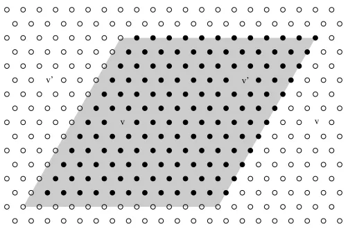
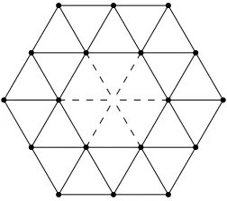
Figure 1. Lattice and the computational domain withN = 12 and two vacancies. The black disks denote the atoms belonging to the computational domainL, the white disks denote the atoms belonging toL#_{\ L, and the vacancies are denoted byv andv}0_.

Lemma 2.1 motivates the splitting of lattice sums into hexagonally symmetric sets. In these calculations the following two identities will prove useful. Their proofs are given in Appendix A.

Lemma 2.2. Let G∈R2×2, andr∈R2,|r|= 1; then

6 X

j=1 GQ

j 6r

2

= 3|G|2_{, and}

(2.1)

6 X

j=1

(Qj₆r)>G(Qj₆r)2

= 3 2|G

sym

|2+3 4|trG|

2_.

(2.2)

Throughout the paper we fix a periodicity parameter N ∈ N. We say that a set A ⊂ R2 is N-periodic if A+NL# = A. For any set A ⊂ R2 we denote its periodic continuation byA#=A+NL#. If A is a family of sets, then we define

A#_={A#_:A∈A}.

We denote the continuous and discrete cells by

Ω :=A6(0, N]2 and L:=L#∩Ω.

We fix a set of vacancysites_V⊂_L and define thediscrete computational domain

as (cf. Figure 1)

L:=L\V.

Ahomogeneous deformationofL#_{is a mapy}

B:L#→R2defined, forB∈R2×2+ ,

asyB(x) :=Bx,x∈ L#. The space of periodic displacementsis denoted by

U =

u:L#_→

R2:u(x+Naj) =u(x) forx∈ L#andj= 1,2 .

A map y :L#_→

invertibility condition we define

µa(y) = inf

x6=x0_∈L#

|y(x0_)−y(x)|

|x−x0_|

and denote

YB:=

y:L#_→

R2:y−yB ∈U andµa(y)>0 , and Y :=S

B∈R2×2+ YB.

2.2. Bonds. Abondis an ordered pair (x, x0)∈L#×L#,x6=x0. When convenient we identify the bondb= (x, x0) with the line segment conv{x, x0}, for example, to integrate over the segment, and correspondingly define |b| :=|x−x0|. The set of bonds between atoms in the computational domainLand all other atoms is denoted by

B:=

(x, x0)∈ L × L#_:x6=x0 _.

The direction of a bond b will be denoted by rb, that is b = (x, x+rb) for some x∈_L#_.

For a mapv:_L#_→

Rk and a bondb= (x, x+rb), we define the finite difference operators

(2.3) Dbv:=Dr_bv(x) :=v(x+rb)−v(x).

With this notation, we haveµa(y) = minb∈B|Dby|/|b|.

We define the set ofallbonds, including vacancy sites, by

B:=(x, x+r) :x∈L, r∈L∗ .

2.3. The interaction potential. Letϕ∈C2(0,+∞) be an interaction potential, and letφ∈C2(R2\ {0}) be defined asφ(r) :=ϕ(|r|). Theinternal atomistic energy of a deformationy∈Y is given by

Ea(y) = X

b∈B φ(Dby) (2.4)

= X

x∈L X

x0_∈L#_\{x}

ϕ |y(x0)−y(x)| .

(2.5)

It is crucial in our analysis thatφ(r) and its derivatives decay rapidly as |r| →

+∞. For example, our analysis is invalid for the slowly decaying Coulomb interac-tions. To avoid technicalities associated with the interaction decay altogether we assume throughout that there exists a cut-off radiusscut>0 such thatϕ(s) = 0 for

all s≥scut. The most commonly employed intermolecular potentials satisfy this

property.

Despite the existence of a cut-off radius, we will need to quantify the decay within the interaction range. To that end we define

(2.6) M2: (0,+∞)→[0,+∞], M2(s) = sup_r∈R2

|r|≥s

kφ00(r)k,

were φ00 : R2\ {0} → R2×2 denotes the 2nd Frechet derivative of φ, and k · k the operator norm of a matrix. We remark that, written in terms of ϕ, we have

M2(s) = sup_t≥s ϕ00(t)

t2

2

+ ϕ0(t)

t

21/2

.

consistency results remain valid for this general form of the interaction potential, the stability analysis relies more heavily on the specific formφ(r) =ϕ(|r|). Hence, for the purpose of the present paper, we understand (2.4) simply as a convenient replacement for the more conventional notation (2.5).

(b) External forces are often used to model, for example, a substrate or an inden-ter. In order to avoid the additional level of complexity they would introduce, we have decided against incorporating external forces. To obtain non-trivial solutions in our numerical experiments, we have instead allowed for defects in the atomistic

lattice.

2.4. The variational problem. The energy functional Ea is twice continuously

differentiable at every pointy∈Y. We understand the first variationδEa(y) as an

element of U∗, and the second variation δ2_E

a(y) as a linear operator from U to U∗_{, formally defined by}

δEa(y), u

= d

dtEa(y+tu)|t=0, foru∈U, and

δ2Ea(y)u, v

= _dtdhδEa(y+tu), vi|t=0, foru, v∈U.

For some macroscopic strain B ∈ R2×2+ , which shall be fixed throughout, the

atomistic problem is to find

(2.7) ya∈argminEa(YB),

where “argmin” denotes the set of local minimizers. If ya ∈ YB is a solution to

(2.7), then it satisfies the first-order necessary optimality condition

(2.8) hδEa(ya), ui= 0 ∀u∈U.

3. _{A/C Coupling Method}

The a/c method we present is motivated by the quasinonlocal QC method pro-posed in [32] and generalised in [7]. In the case of 1D second-neighbour pair interac-tions these methods take a particularly simple form amenable to rigorous analysis [4, 23, 27]. The generalisation to 2D finite range interactions we present here was first proposed by Shapeev [30]. Generalisations to 1D finite range interactions were independently developed in [15].

3.1. Coarse-grained deformations and displacements. Theatomistic region

is a closed polygonal set Ωa⊂int(Ω), and thecontinuum regionis given by Ωc:=

clos(Ω\Ωa)∩Ω. We assume throughout that all corners of Ωa belong to L, and

thatV⊂int(Ωa).

Let Lc

rep ⊂ L ∩Ωc be a set of finite element nodes, or, in the language of the

quasicontinuum method [21], representative atoms. We assume that the corners of the atomistic region belong to Lc

rep. We also define Larep = L ∩int(Ωa), and

Lrep:=Larep∪ Lcrep.

Let Tc

h be a regular (and shape regular) triangulation of Ωc with vertices

be-longing to (Lc

rep)#, which is extended periodically to a regular triangulation (Thc)#

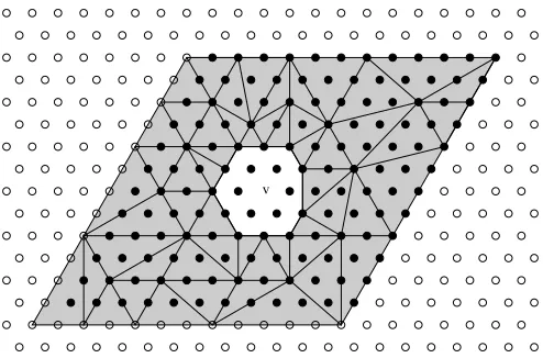
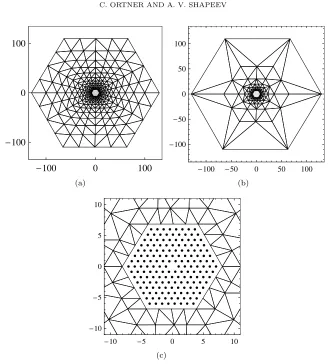
of Ω#_c. An example of such a construction is displayed in Figure 2. We adopt the convention that lattice functions that are piecewise affine with respect to the triangulation (Tc

h)

#_{are understood as piecewise affine functions onall ofΩ}# c , that

is, they may be evaluated at any pointx∈Ω#

c and not only at lattice sites.

For each T ∈ (Tc

h)# we define hT := diam(T), and we define the mesh size

functionh(x) := max{hT :T ∈(Thc)

v

Figure 2. Example of a triangulationThcof the continuum region

Ωc(shaded area), with nodes on∂Ωcare such that the mesh can be

extended periodically to a regular triangulation of Ω#

c. Note that

the boundary of the atomistic region need not be aligned with nearest-neighbour directions.

Whenever we refer to the shape regularity of Tc

h (and later Th), we mean the

ratio between the largest and smallest angle between any two adjacent edges inTh.

We will assume throughout that this is moderate.

We define the set of admissible coarse-grained displacements and deformations, respectively, as

Uh=uh∈U : uh is p.w. affine w.r.t.Thc , YB,h=

yh∈Y :yh−yB ∈Uhandµc(yh)>0 , and Yh=S_B∈R2×2

+ YB,h,

whereµc is defined by

(3.1) µc(yh) := infx,x0∈Ωc

x6=x0

|yh(x)−yh(x0)|

|x−x0_| ≤ess.inf

x∈Ωc

min_r∈R2

|r|=1

|∇yh(x)r|.

Note that, since a continuous interpolant of an invertible atomistic deformation need not necessarily be invertible, we are requiring a more stringent invertibility condition on coarse-grained deformationsyh.

Finally, we define the nodal interpolation operatorIh:U →Uhby

Ihu(x) =u(x) ∀x∈ Lrep,

extended to deformations byIhy−yB=Ih(y−yB), fory∈YB.

3.2. Bond integral formulation. There are two steps in the construction of the a/c method. First, all bonds b that are entirely contained within the continuum region are replaced by line integrals. We collect these bonds into the set

Bc:=

b∈ B: int(b)⊂int(Ω#c) ,

For any functionv that is measurable on the segmentb= (x, x+rb), we define thebond integral

− Z

b

vdb =− Z x+rb

x

vdb =

Z 1

0

v(x+trb) dt.

For any functionvh ∈Uh∪Yh the following one-sided directional derivatives are

well-defined at almost every point ofb= (x, x+r):

∇bvh(x) :=∇rvh(x) := lim

t&0

vh(x+tr)−vh(x)

t .

If x lies in the interior of an element T, thenvh is differentiable at xand hence

∇rvh(x) = (∇vh(x))r. If x lies on an edge or a vertex of the triangulation, the one-sided directional derivative of a continuous piecewise affine function is still well-defined. The directional derivative ∇rvh(x) is only undefined at points x ∈ ∂Ωa

ifr points to the interior of Ωa. For future reference we note the following useful

identity:

(3.2) Dryh(x) =−

Z x+r

x

∇ryhdb, fory∈Y, x∈L#, r∈L∗.

Using this notation we see that if ∇yh has small variation along the bond b, then Dbyh ≈ ∇byh(x) for all x ∈ int(b), and hence we can make the following approximation:

(3.3) φ(Dbyh)≈ −

Z

b

φ(∇byh) db,

which naturally leads to the following definition of an a/c coupling method, which is labelled the ECC method in [30]:

(3.4) Eac(yh) =

X

b∈Ba

φ(Dbyh) + X

b∈Bc − Z

b

φ(∇byh) db.

We will use this formulation of the a/c method in our analysis, however, it does not reduce the complexity of the energy evaluation, which is the purpose of the next section.

It is again easy to see thatEacis twice continuously differentiable inYB,h, for all

B∈_R2×2₊ , and we define the first and second variationsδEac andδ2Eac analogously

toδEa andδ2Ea in§2.4.

3.3. Practical formulation. To make the a/c energy (3.4) “practical”, we need to rewrite it in terms of volume integrals over the Cauchy–Born stored energy density. The tool for achieving this is the bond density lemma [30]. This result is false for general tetrahedra in 3D.

For any polygonal setU ⊂_R2 _{we define itscharacteristic function}

(3.5) χU(x) = lim

t→0

|U∩Bt(x)|

|Bt(x)| forx∈R 2_,

The following result is a reformulation of [30, Lemma 4.4] for the triangular lattice with periodic boundary conditions.

Lemma 3.1 (Bond-Density Lemma). Let T ⊂clos(Ω) be a non-degenerate triangle with vertices belonging toL#, and letr∈L∗, then

X

x∈L − Z x+r

x

χT#db =

1 detA6

|T|.

Proof. A change of coordinates x7→ A6x in [30, Lemma 4.4] yields the following

bond density formula for the full infinite lattice:

X

x∈L# − Z x+r

x

χTdb =

1 detA6

|T|.

Splitting the lattice sum over copies of the cell_L, we obtain

1 detA6

|T|= X

x∈L# − Z x+r

x

χTdb = X

x∈L X

z∈NL# − Z x+z+r

x+z

χTdb.

Upon shifting the integration variable by−z, we can rewrite this as

1 detA6

|T|=X

x∈L − Z x+r

x

X

z∈NL#

χT−zdb = X

x∈L − Z x+r

x

χT#db.

Equipped with the periodic bond-density lemma, we derive a practical formu-lation of the a/c method (3.4). The proof of this result for Dirichlet boundary conditions is contained in [30]; the modifications for the periodic case are straight-forward [25, App. A].

Theorem 3.2. The energy Eac, defined in (3.4), can be rewritten as

Eac(yh) = X

b∈Ba

φ(Dbyh) +

Z

Ωc

W(∇yh) dV + Φi(yh), where

(3.6)

Φi(yh) :=− X

b∈B\Bc − Z

b χ_Ω#

cφ(∇byh) db,

and whereW :_R2×2_→

R∪ {+∞} is the Cauchy–Born stored energy function,

W(F) := 1 detA6

X

r∈L∗

φ(Fr).

3.4. The coarse grained variational problem. To apply the a/c method we compute

(3.7) yac∈argminEac(YB,h).

If yac ∈ YB,h is a solution to (3.7), then it satisfies the first- and second-order necessary optimality conditions

δEac(yac), uh

= 0 ∀uh∈Uh, and

(3.8)

δ2Eac(yac)uh, uh

≥0 ∀uh∈Uh.

(3.9)

Condition (3.9) is insufficient for error estimates; hence we will aim to prove the strongersecond-order sufficient optimality condition

(3.10) δ2Eac(yac)uh, uh

≥γk∇uhk2

L2_(Ω) ∀uh∈Uh

for someγ >0, where the normk∇uhk2

L2_(Ω)is yet to be defined foruh∈Uh. The

choice of norm on the right-hand side of (3.10) is motivated by the fact that the equations (3.8) have a similar structure as finite element discretisations of second-order elliptic equations.

3.5. Brief outline of the error analysis. We give a brief sketch of the main result, Theorem 7.1, to motivate the subsequent technical details that we provide in §5–§7. We stress that this discussion is schematic, and that some steps are not properly defined at this point.

Letyabe a solution of (2.7), andyaca solution of (3.7), and assume thatya, yac,

andIhya are “close” in a sense to be made precise. Suppose, moreover, that (3.10)

holds. Leteh:=Ihya−yac, then we can estimate

γk∇ehk2 L2_(Ω)≤

δ2Eac(yac)eh, eh

≈

δEac(Ihya)−δEac(yac), eh

=hδEac(Ihya), ehi.

The first inequality in the above estimate is the focus of the stability analysis in

§6. The purpose of the consistency analysis§5 is to estimate

δEac(Ihya), eh

≤ Econs_k∇ehk L2(Ω),

which immediately yields ana priorierror estimate:

k∇Ihya− ∇yackL2_(Ω).γ−1Econs.

In §4 we will give an interpretation to∇ya, and establish interpolation error es-timates, so that we can also estimate k∇ya− ∇IhyakL2_(Ω). In §7, we will make

the above arguments rigorous, and in addition establish an error estimate for the energy.

4. _{Auxiliary Results}

4.1. Extension to the vacancy set. A substantial simplification of the subse-quent analysis and notation can be achieved if we extend all function values to the vacancy setV. Other approaches we have considered are significantly more tech-nical and would yield only minor improvements. An altogether different approach might be required to extend the analysis to more general classes of defects.

We define the extension operator as the solution of a variational problem. Let the set of all displacement extensions be given by

UE:=

then, foru∈U, we define

(4.1) Eu:= argmin

v∈UE v=uonL

Φ_Bnn(v), where Φ_Bnn(v) := X

b∈Bnn

rb·Dbv

2

,

where

Bnn:=

(x, x+r) :x∈L, r∈Lnn}

is the set of nearest-neighbour bonds. This definition of the extension operator is motivated by the stability analysis, more precisely, the definition of the vacancy stability indexin§6.1.

For the sake of simplicity of notation, we will identifyEw≡w, except where we need to strictly distinguish the original functionwand its extension.

Proposition 4.1. The variational problem (4.1)has a unique solution, that is, the extension operator E is a well-defined linear operator fromU toUE.

Proof. To prove that (4.1) has a unique solution it is sufficient to show that Φ_Bnn is a positive definite quadratic form on the affine subspace ofUE defined through

the constraintv=uonL. The linearity is a straightforward consequence.

To establish this, we need to employ notation that will be properly defined in

§4.2: letT#

a denote the canonical triangulation of L

#_{, and, for each v ∈U} E, let

¯

v denote the corresponding continuous piecewise affine interpolant. In particular, we then haveDbv=∇b¯v for all bondsb∈Bnn. Applying the bond density lemma,

and (2.2), we obtain

Φ_Bnn(v) =

Z

Ω X

r∈Lnn

r· ∇¯vr

2

dV =

Z

Ω n

3 2

(∇¯v)sym 2

+3 4 tr(∇v¯)

2o

dV.

Since ¯vis fixed in the continuum region, Korn’s inequality shows that Φ_Bnn is indeed coercive.

This proof shows that, in fact,E is defined through the solution of an isotropic linear elasticity problem, with boundary data provided on the edge of a suitably

defined neighbourhood of the vacancy set.

We extend the definition of E to include deformations y ∈ Y, via E(yB +

u) = yB +Eu for all B ∈ R2×2+ . We stress, however, that none of our results

depend (explicitly or implicitly) on the extension of deformations. By contrast, the extension of displacements enters our analysis heavily.

4.2. Micro-triangulation and extension of Tc

h. The triangular latticeL #_has

a “canonical” triangulation T#

a , which is defined so that every nearest-neighbour

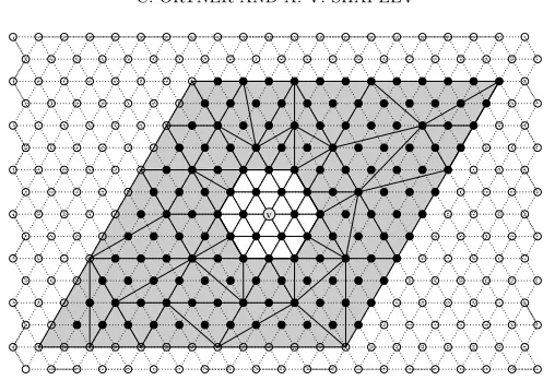
bond is the edge of a triangle; see Figure 3. The subset of trianglesτ ∈ T# a that

are contained in clos(Ω) is denoted by Ta. We will assume throughout that the

following assumption holds, but only cite it explicitly in the main results.

Assumption A. The boundary ofΩais aligned with edges ofTaand the mesh size on∂Ωa is equal to the lattice spacing.

Assumption A implies that any microelementτ ∈ Tamust belong either entirely

to Ωa or to Ωc. This yields a natural extension Th of Thc, which is obtained by

adding all micro-elements τ ∈ Ta, τ ⊂Ωa, so thatTh andTa coincide in Ωa. The

v

Figure 3. The micro-triangulationTa(dotted lines) and the

ex-tension Th of the macro-triangulation to the atomistic domain.

Note that in Ωa,Thcoincides withTaand has no hanging nodes.

the extended mesh Th has no hanging nodes. We emphasize that our subsequent

analysis is valid only for this smaller family of meshes than the a/c coupling method was formulated for (compare Figure 2 with Figure 3).

The definitions of the element sizehT, the mesh size functionh(x), and the shape regularity, from§3.1, are extended toTh andT

# h .

For any lattice functionw:_L#_→

Rkwe define the P1 micro-interpolant ¯w, that is, ¯w∈W1,∞_loc (R2)k and ¯w(x) =w(x) on the lattice sitesx∈L#. In particular, the gradient∇w¯, which is a piecewise constant function, is also well-defined.

Note thatyh∈Yhis interpreted as the continuous P1 interpolant with respect to

the meshTh (themacro-interpolant), while ¯yh is understood as the P1 interpolant

with respect to the meshTa(themicro-interpolant). In our analysis we will require

some technical results comparing ¯yh andyh. Lemma 4.2 gives a global comparison

result, while a local variant is established in Lemma 4.5 below.

Lemma 4.2. Let yh∈Yh, andp∈[1,∞]; then

k∇yh¯ kLp_(Ω)≤CΩ¯ k∇yhk_Lp(Ω),

(4.2)

whereCΩ¯ = max(3(p−2)/(2p),3(2−p)/(2p))≤√3.

Proof. The result follows from an argument analogous to the proof of [22, Lemma

2]. We present the details in [25, App. A].

4.3. W2,∞-conforming interpolants. Smoothness of the atomistic solution in the continuum region is one of the key requirements for error estimates in a/c methods [6, 23]. In previous 1D analyses of a/c methods smoothness was measured via second- and third-order finite differences. A direct extension of this approach is technically and notationally demanding; hence, we propose to measure smoothness of discrete maps in terms of the smoothness of W2,∞-conforming interpolants. In fact, it turns out that our analysis requires no explicit construction, and we therefore define the class of all W2,∞_{-conforming interpolants of deformations y ∈Y}

R2×2+ :

Π2(y) :=y˜∈W2,∞(R2)2: ˜y(x) =y(x) for all x∈L#, and

˜

y(x+Naj) =B(Naj) + ˜y(x) for allx∈R2, j= 1,2 .

Lemma 4.3 (Interpolation Error Estimates). Let p ∈ [1,∞], then there exists a constant Ch, depending only on˜ pand on the shape regularity of Th, such that, for ally∈Y,

(4.3) ∇y˜− ∇Ihy

_Lp_(T)≤ChhT˜

∇2y˜

_Lp_(T) ∀T ∈ Th ∀y˜∈Π2(y). Moreover, there exists a constantCa, depending only on˜ p, such that

(4.4) ∇y˜− ∇y¯

_Lp_(τ)≤Ca˜

∇2y˜

_Lp_(τ) ∀τ∈ Ta ∀y˜∈Π2(y).

Proof. Both estimates are standard [1]. The constant ˜Ca is independent of the

mesh quality sinceTa contains only a single element shape.

Remark 4.1. We show in [25, Remark 4.1], that an explicit W2,∞-interpolant ˜

yhct can be constructed (using, e.g., the Hsieh–Clough–Tocher element) such that

(4.5) c1k∇2yhct˜ kLp_(τ)≤[∇y¯]

_Lp_(Γτ)≤c2k∇ 2

˜

yhctkLp_(ω τ),

where ci > 0 are universal constants, Γτ is the union of all edges of the

micro-triangulation touchingτ,ωτ the union of all micro-elements touchingτ, and where

[∇y¯] denotes the jump of∇y¯across micro-triangulation edges.

The inequalities in (4.5) show a local equivalence between second derivatives of “good” W2,∞-conforming interpolants and jumps of∇w¯, which one might consider

the most natural measure of smoothness.

4.4. Notation for edges. Several estimates in our consistency analysis will be phrased in terms of the jumps of∇yh,yh∈Yh, across element edges, for which we

now introduce the required notation: letF_h#denote the set of (closed) edges of the triangulationT_h#, and let

Fh:=

f ∈ F_h#: int(f)⊂Ω , and Fhc :=

f ∈ Fh:f 6⊂Ωa ,

where, here and throughout, int(f) denotes the relative interior of an edgef. That is, the set Fh includes one periodic copy of all element edges contained in Ω, and

Fc

hexcludes all edges that are subsets of Ωa.

Letf ∈ F_h#,f =T+∩T−,T± ∈ Th, and suppose thatw: int(T+)∪int(T−)→Rk has well-defined tracesw± from T±, then we define the jump [w](x) :=|w+(x)−

w−(x)| for all x ∈ int(f). Whenever we write R_Fc

h

, Lp(Fc

h), etc., we identify F c h

with the union of its elements.

In the next lemma we provide a tool to estimate jumps across edges in terms of smooth interpolants. The proof is given in Appendix A.

Lemma 4.4. Let y∈Y andf ∈ F_h#,f =T+∩T− forT±∈ Th; then

[∇Ihy]

_Lp_(f)≤Cf h1/p

0 ∇2_y˜

_Lp_(T

+∪T−) ∀y˜∈Π2(y), and

(4.6)

[∇Ihy]

_Lp_(Fc

h)

≤Cf31/ph1/p

0 ∇2_y˜

_Lp_(Ωc) ∀y˜∈Π2(y).

whereCf depends only on the shape regularity ofTh.

4.5. Micro- and macro-interpolants. The following local version of Lemma 4.2 and its corollary, Lemma 4.6, are motivated by gradient jumps estimates of Lemma 4.4. The proof of Lemma 4.5 is given in Appendix A. We remark that the constant

¯

Cais fairly moderate as the discussion at the end of the proof shows.

Lemma 4.5. Let yh∈Yh,τ ∈ Ta, andp∈[1,∞]; then

(4.8) k∇y¯hkLp_(τ)≤C¯_a

k∇yhk

p Lp_(τ)+

[∇yh]

p Lp_(F#

h∩int(τ))

1/p ,

whereC¯a depends only on the shape regularity ofTh.

Combining Lemma 4.5 and Lemma 4.3, we obtain the following result, which is a critical ingredient of the analysis in§5.1.

Lemma 4.6. Let y∈Y andp∈[1,∞]; then

(4.9) ∇y¯− ∇Ihy _Lp_(Ω

c)≤

¯

CIh

h∇2y˜

_Lp_(Ω

c) ∀y˜∈Π2(y),

whereCI¯_h depends only on the shape regularity ofTh.

Proof. We cannot immediately use the interpolation error estimates (4.3) and (4.4) to estimate the termk∇(¯y−Ihy)kLp_(Ω), due to the occurrence ofIhy. Instead, we

first fix a micro-element τ ⊂Ωc, define z(x) := (∇y¯|τ)x for all x∈ R2, and use (4.8) to estimate

∇(¯y−Ihy) p Lp_(τ)=

∇Ih(y−z) p Lp_(τ)

≤C¯_aph∇Ih(y−z) p Lp_(τ)+

[∇Ih(y−z)] p Lp_(Fc

h∩int(τ))

i

= ¯C_aph∇(Ihy−y¯) p Lp_(τ)+

[∇Ihy]

p Lp_(Fc

h∩int(τ))

i .

We will next sum this estimate for allτ∈ Ta. Using the fact that ¯y=Ihyin Ωa,

as well as the interpolation error estimates (4.3) and (4.4), and the jump estimate (4.7), we obtain, for any ˜y∈Π2(y),

∇(¯y−Ihy)

_Lp_(Ω)≤Ca¯

h

∇(Ihy−y¯) _Lp_(Ω

c)+

[∇Ihy]

_Lp_(Fc

h)

i

≤Ca¯ h∇(Ihy−y˜) _Lp_(Ω

c)+

∇(˜y−y¯) _Lp_(Ω

c)+

[∇Ihy]

_Lp_(Fc

h)

i

≤Ca¯ hCh˜ kh∇2_y˜k

Lp_(Ωc)+ ˜Cak∇2y˜k_Lp_(Ωc)+Cf31/pkh1/p

0 ∇2_y˜k

Lp_(Ωc)

i .

Sinceh≥1, the stated result follows.

5. _Consistency

Recall from our preliminary discussion in §3.5 that the total consistency error

associated with the atomistic solutionya is

δEac(Ihya)k_W−1,p h

=δEac(Ihya)−δEa(ya) _W−1,p

h

=:Econs p (y

a_),

where, for Ψ∈U∗

h, the negative Sobolev norm is defined as

kΨk_W−1,p h

:= sup

uh∈Uh k∇uhk_Lp0(Ω)=1

Ψ, uh

In this section we prove the following estimate. Our assumption thatφhas a finite cut-off radius (see§2.3) guarantees thatCconsis finite.

Theorem 5.1 (Consistency). Suppose that Assumption A holds. Let y ∈ Y

such that µa(y)>0and µc(Ihy)>0. Then, for eachp∈[1,∞], we have

(5.1) Econs

p (y)≤Ccons inf ˜ y∈Π2(y)

kh∇2_y˜k Lp(Ωc),

whereCconsdepends only onµa(ya), onµc(Ihy), and on the shape regularity ofTh.

Outline of the proof. To prove this result, we first split the consistency error into a

coarsening errorand amodelling error:

Epcons(y) =

δEac(Ihy)−δEa(y) _W−1,p

h

≤

δEac(Ihy)−δEa(Ihy) _W−1,p

h

+δEa(Ihy)−δEa(y) _W−1,p

h ,

=:Emodel p (y) +E

coarse p (y).

We note that, since we estimate the modelling error at the interpolant Ihy, the mesh dependence is not entirely removed fromEmodel_.

The estimate for the coarsening error is given in Lemma 5.4, and the estimate for the modelling error in Lemma 5.9, which together yield (5.1) with Ccons =

Ccoarse+Cmodel. Note that we have ignored the improved mesh size dependence of the modelling error, and estimated 1≤hto obtainEmodel

p (y)≤Cmodelkh∇2y˜kLp_(Ω

c)

for all ˜y∈Π2(y).

Remark 5.1. The details of the proof of Theorem 5.1 are technically involved, due to the relatively weak assumptions that we made on the meshTh, as well as

the fact that we insisted to estimate the consistency error in terms ofkh∇2_y˜k Lp(Ωc)

only. A simplified argument can be given if weaker estimates are sufficient; see [25,

App. B].

5.1. Coarsening error. The ingredients in the coarsening error estimate are a local Lipschitz bound on δEa, and the interpolation error estimate of Lemma 4.6.

We begin by stating a useful auxiliary result.

Lemma 5.2. Let r∈L∗, q∈[1,∞), uh∈Uh andu∈U, then

X

x∈L

Druh(x) q

≤X

x∈L − Z x+r

x

|∇ruh|q_{db =} 1

detA6k∇ruhk

q

Lq_(Ω), and

(5.2)

X

x∈L Dru(x)

q

≤X

x∈L − Z x+r

x

|∇ru¯|qdb =_det1_A6k∇ru¯k q Lq_(Ω).

(5.3)

Proof. The result is a straightforward application of the bond density lemma. We give the proof for (5.2), since (5.3) is a particular case.

Jensen’s inequality implies the inequality in (5.2):

Druh(x) q

=

− Z x+r

x

∇ruhdb q

≤ − Z x+r

x ∇ruh

q

Using the fact that that {χ#_T :T ∈ Th} is a partition of unity, continuity of ∇ruh

across faces with directionr, and Lemma 3.1, we have

X

x∈L − Z x+r

x

|∇ruh|q_{db =} X T∈Th

X

x∈L − Z x+r

x

χT#|∇ruh|qdb

= X

T∈Th

|∇ruh|T|q X

x∈L − Z x+r

x

χT#db

= 1

detA6 X

T∈Th

|T||∇ruh|T|q.

The next auxiliary result is a Lipschitz bound onδEa.

Lemma 5.3. Let y, z∈Y, andµ:= min{µa(y), µa(z)}>0; then

(5.4)

δEa(y)−δEa(z), uh≤CL

∇y¯− ∇z¯

_Lp_(Ω)k∇uhkLp0(Ω)

for all uh ∈ Uh, where CL = CL(µ) := _det1_A6P_r∈L∗|r|2M2(µ|r|). The result remains true if uh is replaced with u∈U, and∇uh with ∇u.¯

Proof. Fixuh∈Uh andp∈(1,∞); then

δEa(y)−δEa(z), uh

≤ X

b∈B

φ0(Dby)−φ0(Dbz) |Dbuh|

≤ X

b∈B M_|b|0

Dby−Dbz |b|

Dbuh |b|

,

where M_ρ0 = M2(µρ)ρ2_{. Let w = y−z, then, applying a H¨older inequality, we}

obtain that

δEa(y)−δEa(z), uh

≤

X

b∈B

M_|b|0 D_|b|bw

p1/pX

b∈B

M_|b|0 Db_|b|uh

p01/p

0

.

Each of the two groups can be estimated using Lemma 5.2, for example,

X

b∈B

M_|b|0 D_|b|bw p

≤ X

b∈B

M_|b|0 D_|b|bw p

= X

r∈L∗

M_|r|0 |r|−pX x∈L Drw(x)

p

≤ X

r∈L∗

M_|0_r| detA6|r|

−p_k∇ rw¯k

p

Lp_(Ω)=k∇w¯k p Lp_(Ω)

X

r∈L∗

M_|0_r| detA6.

By the same argument, using (5.2) instead of (5.3), we obtain

X

b∈B

M_|b|0 D_|b|buh p0

≤ 1

detA6

X

r∈L∗

M_|r|0 k∇uhk p0 Lp0_(Ω).

This establishes (5.4) for p∈(1,∞). The cases p∈ {1,∞} are obtained with minor modifications of the above argument. The proof foru∈U is analogous.

We can now formulate the coarsening error estimate.

Lemma 5.4. Let y∈Y andµ:= min(µa(y), µa(Ihy))>0; then,

(5.5) Epcoarse(y)≤C

coarse h∇2y˜

Lp_(Ωc),

Proof. According to Lemma 5.3 we have

δEa(y)−δEa(Ihy), uh

≤CL∇(¯y−Ihy)

_Lp_(Ω)k∇uhkLp0_(Ω).

From Lemma 4.6 we obtain that

k∇(¯y−Ihy)kLp_(Ω)≤C¯_Ih

h∇2y˜

_Lp(Ω

c) ∀y˜∈Π2(y),

which yields (5.5) withCcoarse_=CLCI¯

h.

Remark 5.2. With an alternative splitting of the consistency error (see, e.g., [27, 22]) it would have been necessary to estimate the coarsening error whenEa is

replaced withEac. In that case, we would have needed a Lipschitz estimate onδEac.

DefiningEac(¯y) in a canonical way, our proof above is easily modified to yield

δEac(Ihy)−δEac(¯y), uh

≤

X

b∈Ba

M_|b|0 − Z

b

∇bIhy− ∇by¯ p

db

+X

b∈Bc

M_|b|0 − Z

b

∇bIhy− ∇by¯ p

db

1/p

C_L1/p0k∇uhk_Lp0.

The first group we can again convert into volume integrals and estimate using Lemma 4.6. However, the second group contains integrals over both macro- and micro-interpolants, and therefore cannot be converted into volume integrals using the bond density lemma.

However, as we show in [25, App. B], weaker (though technically less involved)

estimates can be obtained in this way.

5.2. Modelling error. For the majority of the modelling error analysis we can replaceIhy by an arbitrary discrete deformationyh ∈Yh. Hence, we fix yh ∈Yh

such thatµ:= min(µa(yh), µc(yh))>0. Moreover, we fix constantsar>0,r∈_L∗,

which will be determined later,ab:=ar_b for all bondsb∈_B, andM_ρ0 :=M2(µρ)ρ2

for allρ >0.

With this notation, and using (3.2), we have

δEac(yh)−δEa(yh), uh

= X

b∈Bc − Z

b

φ0(∇byh)· ∇buhdb−X

b∈Bc

φ0(Dbyh)·Dbuh

= X

b∈Bc − Z

b

φ0(∇byh)−φ0(Dbyh)

· ∇buhdb

≤ X

b∈Bc

M2(µ|b|)− Z

b

∇byh−Dbyh

|∇buh|db

= X

b∈Bc

M_|b|0 − Z

b

a−1_b |b|−1

∇byh−Dbyh

ab|b|−1|∇buh|

Following a similar procedure as in the proof of Lemma 5.3 (applying a H¨older inequality and Lemma 5.2), we obtain

δEac(yh)−δEa(yh), uh

≤

X

b∈Bc

M_|b|0 |b|−pa−p_b − Z

b

∇byh−Dbyh p

db

1/p C1/p

0

1 k∇uhkLp0_(Ω)

=:C₁1/p0e(yh)k∇uhkLp0_(Ω),

(5.6)

whereC1=_det1_A

6

P r∈L∗M

0 |r|ap

0

r, and where

e(yh)p := X

b∈Bc

M_|b|0 |b|−p_a−p

b eb(yh)p,

eb(yh)p :=− Z

b

∇byh−Dbyh p

db.

(5.7)

We will estimate the termseb(yh)p in terms of the jumps of∇yh. To that end,

we define the jump sets

(5.8) J(b) :=f ∈ Fh: #(f∩int(b)) = 1 .

Faces parallel tob are ignored since the directional derivative ∇rbyh is continuous

across these faces. For eachf ∈J(b) we define the weights

wb,f :=

1, iff∩int(b)⊂int(f),

1/2, otherwise;

that is,wb,f = 1 ifbcrosses f in its relative interior, andwb,f = 1/2 ifb crossesf

at one of its endpoints. Finally we define the quantities

(5.9) nj(b) :=

X

f∈J(b)

wb,f, and nj(r) := max b∈Bc

rb=r nj(b).

Lemma 5.5. Let b∈ Bc, then

(5.10) eb(yh)p≤nj(b)p−1 X

f∈J(b)

wb,f[∇byh]f p

.

Proof. Define ψ(t) = ∇byh(x+trb) and let Jψ ⊂(0,1) be the set of jumps of ψ,

then

(5.11) eb(yh)p=

Z 1

0

ψ(t)− Z 1

0

ψ(s) ds p

dt.

For any pointt∈(0,1)\Jψ we can estimate

ψ(t)− Z 1

0

ψ(s) ds

≤ Z 1

0

ψ(t)−ψ(s) ds≤

Z 1

0 Z

r∈(t,s)

|ψ0|drds

≤ Z 1

0

|ψ0|dr= X

r∈Jψ

where|ψ0|dris understood as the measure that represents the distributional deriv-ative ofψ. Inserting this estimate into (5.11), yields

eb(yh)p ≤

X

r∈Jψ

|ψ(r+)−ψ(r−)| p

≤(#Jψ)p−1 X

r∈Jψ

ψ(r+)−ψ(r−) p

,

which translates directly into (5.10), in the case thatbdoes not intersect any faces in their endpoints.

Ifbdoes intersect certain faces in endpoints then one replaces the path{x+trb:

t∈(0,1)} by two paths that “circle” around the endpoints, each weighted with a

factor 1/2.

Recall the detail of the definition of Fc

h from §4.4. Since only bonds b ∈ Bc

contribute to the consistency error, it follows that only jumps across facesf ∈ Fc h

occur in the following estimate. Interchanging the order of summation, we obtain

e(yh)p ≤ X

b∈Bc

M_|b|0 |b|−pa−p_b nj(b)p−1 X

f∈J(b)

wb,f[∇byh]f p

≤ X

r∈L∗

M_|r|0 |r|−p_a−p

r nj(r)p−1 X

b∈Bc

rb=r

X

f∈J(b) wb,f

[∇byh]f

p

= X

r∈L∗

M_|r|0 |r|−pa−p_r nj(r)p−1 X

f∈Fc

h

ncross(f, r) [∇ryh]f

p

,

(5.12)

wherencross(f, r) is the (weighted) number of bondsbwith directionrand crossing the facef; more precisely,

ncross(f, r) := X

b∈Bc,rb=r f∈J(b)

wb,f.

Lemma 5.6. Let f ∈ Fc

h andr∈L∗; then

(5.13) ncross(f, r)≤ 1

detA62|r|length(f).

Proof. Letf ={z+ts:t∈[0,1]}, and define the parallelogram

P ={z+t1s+t2r:t1∈[0,1], t2∈(−1,1)},

then we have

ncross(f, r) = X

b∈Bc,rb=r f∈J(b)

− Z

b

χPdb≤ X

x∈L# − Z x+r

x

χPdb = det1A6|P|,

where, in the last equality, we have used the fact thatPis the union of two triangles, which implies that the bond density lemma holds forPas well. To obtain the result

we simply note that|P| ≤2|r|length(f).

Estimate (5.13) and|[∇ryh]f| ≤ |r||[∇yh]f|yield

(5.14) e(yh)p≤C2

X

f∈Fc

h

hf[∇yh]f

p ,

whereC2=_det1_A

6

P

r∈L∗2M

0

Choosing the constantsar so thatC1=C2,

2|r|a−pr nj(r)p−1=ap

0

r = (2|r|)1/pnj(r)1/p

0

,

we obtain

(5.15) C1=C2= _det1_A

62

1/p X r∈L∗

M2(µ|r|)|r|2+1/p_nj(r)1/p0_.

To obtain a more explicit constant, we estimatenj(r) next. The following result is unsurprising, but its proof rather technical; hence we have postponed it to Appendix A.

Lemma 5.7. There exists a constant Cnj, which depends only on the shape

regularity ofTh, such that

(5.16) nj(b)≤Cn_j(|b|+ 1) ∀b∈ Bc.

Combining (5.14), (5.15), and (5.16), we deduce the following intermediate result, which is interesting in its own right, since it could serve as a basis fora posteriori

error estimates.

Lemma 5.8. Let yh∈Yh,µ:= min(µa(yh), µc(yh))>0; then

(5.17)

δEac(yh)−δEa(yh), uh≤C1model [∇yh]

_Lp_(Fc

h)

k∇uhk_Lp0_(Ω)

for alluh∈Uh, whereC1model=C0 P

r∈L∗Mr(µ|r|)|r|

3 _andC0 _{depends only on the}

shape regularity of Th.

Applying Lemma 4.4 to estimate k[∇yh]kLp_(Fc

h) in (5.17), we obtain the final

modelling error estimate.

Lemma 5.9 (Modelling Error). Let y∈Y and suppose that

µ:= min(µa(Ihy), µc(Ihy))>0;

then

(5.18) Epmodel(y)≤C

model h1/p

0 ∇2y˜

Lp_(Ωc),

where Cmodel _=CP

r∈L∗M2(µ|r|)|r|

3 _{and C depends only on the shape regularity}

of Th.

Remark 5.3. At first glance it may seem that the termsk[∇yh]kLp_(Fc

h) in (5.17)

andkh1/p0_∇2_y˜k

Lp_(Ωc)in (5.18) are not scale invariant. This is, however, deceiving.

Since the atomic scale is 1 in our case, one should read (5.18) as

h1/p

0 ∇2_y˜

_Lp_(Ω

c)=

11/ph1/p

0 ∇2_y˜

_Lp_(Ω

c),

which is again scale invariant if 1 is scaled in the same way ash. Indeed, it can be checked that, had we formulated the entire analysis with scaled quantitiesx→εx,

y→εy, andP

→ε2P_{, then we would have obtained}

kε1/p_h1/p0_∇2_y˜k Lp_(Ω

6. Stability

6.1. Main results. The most natural notion of stability for variational problems is positivity of the second variation (at certain deformations of interest).

We first state the main stability result for the case of a homogeneous deformation and_V=∅. This serves as reference point and motivation for the general stability result below, which has a more involved formulation.

Theorem 6.1. Suppose that Assumption A holds, and that_V=∅. LetB∈_R2×2₊

with singular values0< m≤M; then

δ2Eac(yB)uh, uh

≥γhomkB>∇uhk2L2_(Ω) ∀uh∈Uh,

whereγhom=γhom(m, M) := min(3₄c+9₄c⊥,9₄c+3₄c⊥),

c(⊥)=c(⊥)(m, M) := _det1_A

6

P∞ n=1c

(⊥)

n , and

cn:= (

min_s∈[m,M] ϕ00_s(s)2 , n= 1,

0∧mins∈[m,M]`

2

nϕ

00_(s`

n)

s2 , n >1,

c⊥n := (

min_s∈[m,M] ϕ_s0(s)3 , n= 1,

0∧mins∈[m,M]`nϕ

0_(s`

n)

s3 , n >1.

(6.1)

Theorem 6.1 is a special case of Theorem 6.2 below, restricted to homogeneous lat-tices without defects. A direct proof can be given by first specializing the definition of H(yh) in (6.11) toyh =yB andV=∅, and then applying Lemma 6.4, withH replaced withH(yB).

Our generalisation to defects uses the concept of avacancy stability index. Using the extension operatorE:U →UE (see§4.1) we define

κ(_V) := maxnk >0 : X

b∈Bnn

rb·Dbu

2

≥k X

b∈Bnn

rb·DbEu 2

foru∈Uo.

(6.2)

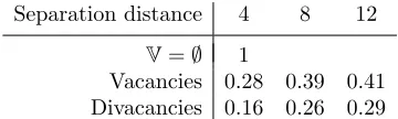
We present numerically computed lower bounds on κ(_V) in Table 1, and in §6.7 rigorously prove the boundκ(_V)≥2/7 if_Vconsists of separated vacancies.

Remark 6.1 (Optimality of the extension operator). Recall the definition of Φ_Bnn from§4.1, and let ΦBnn be defined analogously, then (6.2) can be rewritten

as

κ(V) = max

n

k >0 : ΦBnn(u)≥kΦBnn(Eu) for allu∈U

o .

SinceEuis chosen to minimize the value of Φ_Bnn(Eu), it gives the largest possible stability index among all possible extensions.

Moreover, we can characteriseκ(_V) in terms of an operator norm of E. LetU be equipped with the norm p

ΦBnn and UE with the norm

p

Φ_Bnn, then κ(_V) =

infu∈U\{0}ΦΦBBnnnn(Eu)(u)

=kEk−2_L(U,U

Separation distance 4 8 12

V=∅ 1

Vacancies 0.28 0.39 0.41 Divacancies 0.16 0.26 0.29

Table 1. Numerically computed lower bounds on vacancy stabil-ity indices (rounded down to two significant digits) whenVconsists of either single vacancies, or divacancies separated by “separation distance”.

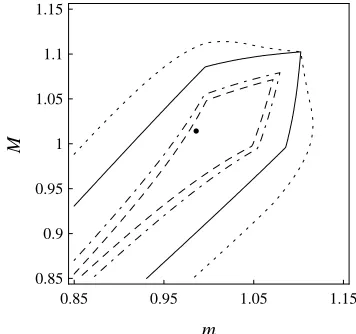
To state the main stability result, we define a family of regions in the space of deformations: for 0< m≤M and ∆>0 let

SB,h(m, M,∆) :=

yh∈YB,h: µa(yh)≥mandµc(yh)≥m;

|Dbyh| ≤M|b| ∀b∈ Baandk∇yh|Tk ≤M ∀T ∈ Thc;

|B−1Dbyh−rb| ≤∆|b| ∀b∈ Ba andkB−1∇yh|T −1k ≤∆ ∀T ∈ Thc .

Theorem 6.2. Suppose that Assumption A holds and suppose thatyh∈SB,h(m, M,∆) for0< m≤M and0≤∆≤p

κ(V)/2; then

δ2Eac(yh)uh, uh

≥γkB>∇uhk2

L2_(Ω) for alluh∈Uh,

whereγ=γ(m, M,∆, κ(_V))is defined by (6.32), and by (6.35)–(6.38).

Theorem 6.2 is our main stability result for nonlinear deformations with defects. Its proof is contained in§6.2–§6.6. In§6.2 we estimateδ2Eac below by an operator

Hthat localizes all finite differences of test functions. In§6.3 we use a perturbation argument to reduce the problem to a homogeneous deformation with a defect. In

§6.4 we employ the definition of the stability index to reduce the problem to one without defect, which is then analyzed in §6.5. In the perturbation argument we introduce several free parameters, which are finally optimized in§6.6.

In §6.8 we will investigate the range of parameters for which γ > 0, and in particular show numerically that non-trivial solutions exist to which Theorem 6.2 applies.

6.2. Stability proof 1: a general lower bound. The representation (3.4) of the a/c energyEac yields the following expression for the second variationδ2Eac:

hδ2Eac(yh)uh, uhi= X

b∈Ba

Dbu>hφ00(Dbyh)Dbuh

+X

b∈Bc − Z

b

∇bu>_hφ00(∇byh)∇buhdb,

(6.3)

for alluh∈Uh, where we recall thatφ00(r) is understood as the Hessian matrix of φ. A straightforward calculation shows thatφ00 can be written, in terms ofϕ0 and

ϕ00, as

(6.4) φ00(r) =ϕ00(|r|)r |r|⊗

r |r|+

ϕ0(|r|) |r| 1−

r |r|⊗

r |r|

We will use the fact that_|r|r ⊗r

|r|is the orthogonal projection onto the space span{r}

and that (1− r |r|⊗

r

|r|) is the orthogonal projection onto span{r} ⊥

. Recalling the notationa×b= (Q4a)·b, whereQ4denotes a rotation through angleπ/2, we have

h> r |r|⊗

r |r|)h=

h·_|r|r

2

, and h> 1− r |r|⊗

r |r|

h=

h×_|r|r 2

.

Hence, we can rewrite (6.3) as

hδ2Eac(yh)uh, uhi

= X

b∈Ba

n_ϕ00_(|D

byh|)

|Dbyh|2 |Dbyh·Dbuh|

2₊ϕ0(|Dbyh|)

|Dbyh|3 |Dbyh×Dbuh| 2o

(6.5)

+X

b∈Bc − Z

b n_ϕ00_(|∇

byh|)

|∇byh|2 |∇byh· ∇buh|

2₊ϕ0(|∇byh|)

|∇byh|3 |∇byh× ∇buh| 2o_db.

Next, we construct a relatively crude lower bound on the Hessian δ2_E

ac, which

will nevertheless be sufficient to obtain stability estimates in a range of interesting deformations. Our goal is to “localise” the finite differences Dbuh occurring in the Hessian representation (6.5), and to render the scalar coefficients hexagonally symmetric.

Sinceyh∈SB,h(m, M,∆), we can estimate the coefficients in (6.5) by

ϕ00(|Dbyh|)

|Dbyh|2 ≥C|b| and

ϕ0(|Dbyh|) |Dbyh|3 ≥C

⊥

|b|, forb∈ Ba,

with analogous estimates forb∈ Bc, where

Cρ:=

(

min_s∈[m,M] ϕ_(ρs)00(ρs)2 , ρ= 1,

0∧mins∈[m,M] ϕ

00_(ρs)

(ρs)2 , ρ >1,

and

C_ρ⊥:=

(

mins∈[m,M] ϕ0_(ρs)

(ρs)3 , ρ= 1,

0∧mins∈[m,M] ϕ

0_(ρs)

(ρs)3 , ρ >1.

(6.6)

We note that these lower bounds are independent of yh, and moreover, all coeffi-cients for non-nearest neighbour bonds are non-positive.

With this notation, we obtain from (6.5) that

hδ2Eac(yh)uh, uhi ≥ X

b∈Ba

n

C|b||Dbyh·Dbuh|2+C|b|⊥|Dbyh×Dbuh|2 o

+X

b∈Bc − Z

b n

C_|b||∇byh· ∇buh|2+C|b|⊥|∇byh× ∇buh|2 o

db.

(6.7)

We now observe that we have constructed the extended meshThin such a way that

in the atomistic region every nearest-neighbour bondb∈ Bnn lies on the edge of a

triangle. As a result we have the identity

(6.8) Dbuh=∇buh(x) for allx∈int(b), for allb∈ Ba∩ Bnn,

which we will use heavily throughout. In particular, this implies that

X

b∈Bnn∩Ba

n

C1|Dbyh·Dbuh|2_+C⊥

1 |Dbyh×Dbuh|2 o

(6.9)

= X

b∈Bnn∩Ba − Z

b n

C1|Dbyh· ∇buh|2+C1⊥|Dbyh× ∇buh|2 o

Our second observation is that, since C|b|, C|b|⊥ ≤0 for b∈ Ba\ Bnn we can use

(3.2) and Jensen’s inequality to estimate

X

b∈Ba\Bnn

n

C|b||Dbyh·Dbuh|2+C|b|⊥|Dbyh×Dbuh| 2o

= X

b∈Ba\Bnn

n C|b|

Dbyh·− R

b∇buhdb 2

+C_|b|⊥Dbyh×− R

b∇buhdb

2o

≥ X

b∈Ba\Bnn − Z

b n

C|b|

Dbyh· ∇buh 2

+C_|b|⊥Dbyh× ∇buh

2o

db.

(6.10)

Inserting (6.9) and (6.10) into (6.7) we obtain the following estimate:

δ2Eac(yh)uh, uh≥ hH(yh)uh, uhi

:= X

b∈Bc − Z

b n

C_|b||∇byh· ∇buh|2+C|b|⊥|∇byh× ∇buh|2 o

db (6.11)

+ X

b∈Ba − Z

b n

C|b||Dbyh· ∇buh|2+C|b|⊥|Dbyh× ∇buh|2 o

db,

whereC|b|, C|b|⊥ are defined in (6.6).

6.3. Stability proof 2: the perturbation argument. In the next step, we will estimate the effect of replacingDryhand∇ryh withBr. To that end, the following lemma will be helpful.

Lemma 6.3. Suppose that yh ∈SB,h(m, M,∆); then, for allg ∈R2, x∈Ω, r ∈ R2, and for all possible choices ofα >0,

(6.12) |∇ryh(x)·g| 2

− |Br·g|2 ≤α

Br·g

2

+ 1 + _α1∆2|r|2|B>g|2.

Similarly, for all g∈_R2_{, x∈ L, r∈}

L∗, andα >0, we have

(6.13) |Dryh(x)·g|2− |Br·g|2 ≤α

Br·g

2

+ 1 + 1_α

∆2|r|2_|B>_g|2_.

The same inequalities hold if “·” is replaced with “×”.

Proof. We verify the bound (6.12) by a straightforward algebraic manipulation (suppressing the argumentx), usingkB−1∇yh−1k ≤∆:

|∇ryh·g|2− |Br·g|2

=

(|∇ryh·g|+|Br·g|) (|∇ryh·g| − |Br·g|) ≤(|(∇ryh−Br)·g|+ 2|Br·g|)|(∇ryh−Br)·g|

≤2|Br·g|∆|r||B>g|+ ∆2|r|2_|B>_g|2_.

Applying a weighted Cauchy inequality 2ab≤αa2+α−1b2 we obtain (6.12). The proofs of (6.13), and of the inequalities where “·” is replaced with “×” are analogous.

Applying Lemma 6.3 to the operator H(yh), defined in (6.11), we obtain, for constantsα|b|, α⊥|b|>0,

hH(yh)uh, uhi ≥ hH(yB)uh, uhi

(6.14) −X b∈B − Z b n

α|b||C|b||

Brb· ∇buh 2

+α⊥_|b||C_|b|⊥|

Brb× ∇buh

2o

db

−∆2X

b∈B

|b|2n _{1 +} 1 α|b|

|C_|b||+ 1 + 1 α⊥

|b|

|C_|b|⊥|o− Z

b B>∇buh

2

db,

for all yh ∈ SB,h(m, M,∆) and uh ∈ Uh. Note that, in the third term, we have

estimated the sum over Bbelow by the sum overB. We also remark that, for the time being, we retain maximal flexibility in our choice of the constantsα|b|andα⊥|b|.

We will (partially) optimize over all possible choices in the last step of our proof. From here on, to simplify the notation, we define the transformed displacement

vh:=B>uh.

This means that we can replace (Brb· ∇buh) by (rb· ∇bvh), and so forth.

Since the algebraic structure of the first and second term in (6.14) is identical it is natural to combine them. Hence, we define

hH˜uh, uhi:= X

b∈B − Z b n ˜ C|b|

rb· ∇bvh 2

+ ˜C_|b|⊥rb× ∇bvh

2o

db,

(6.15)

hL˜uh, uhi:= X

b∈B

|b|2n _{1 +} 1 α|b|

|C|b||+ 1 +_α1⊥ |b|

|C_|b|⊥|o− Z b ∇bvh 2 db,

where ˜Cρ(⊥):=Cρ(⊥)−α(⊥)ρ |Cρ(⊥)|. (Here and throughout the superscript (⊥), e.g.,

inCρ(⊥), is used to refer simultaneously toCρ orCρ⊥.)

Employing the periodic bond-density lemma, the decomposition of the triangular lattice described in Lemma 2.1, and the definition of the constantsc(⊥)n :=`4nC

(⊥) `n ,

the operatorL˜can be rewritten as

hL˜uh, uhi= ( ˜L+ ˜L⊥)k∇vhk2

L2_(Ω), where

˜

L(⊥)=_det3_A

6

P∞

n=1 1 + 1/α (⊥) `n

|c(⊥)_n |.

(6.16)

In summary, we have obtained that, ifyh∈SB,h(m, M,∆), then

(6.17) hδ2Eac(yh)uh, uhi ≥ hH˜uh, uhi −∆2( ˜L+ ˜L⊥)k∇vhk2L2,

for alluh∈Uh, where ˜His defined in (6.21), and and ˜L(⊥)in (6.16).

6.4. Stability proof 3: extension toB. In the next step, we apply the extension operator (see§4.1) and the definition of the stability indexκ:=κ(V) (see§6.1).

Distinguishing whether ˜C1 is positive or negative, and using the definition ofκ

in the first case, we obtain

X

b∈Bnn

˜

C1rb·Dbvh 2 ≥ ( κP b∈Bnn

˜

C1rb·Dbvh 2

, C1˜ ≥0, P

b∈Bnn

˜

C1rb·Dbvh 2

, C1˜ <0,

which can be rewritten as

(6.18) X

b∈Bnn

˜

C1− Z

b

rb· ∇bvh 2

db≥min( ˜C1, κC˜1) X

b∈Bnn − Z

b

rb· ∇bvh 2

For the “perpendicular” nearest-neighbour terms the same argument (we now need to use (6.2) withu=Q>4B>uh=Q>4vh) yields

(6.19) X

b∈Bnn

˜

C₁⊥− Z

b

|rb× ∇bvh|2_{db≥min( ˜C}⊥ 1, κC˜

⊥ 1)

X

b∈Bnn − Z

b

|rb× ∇bvh|2_db.

Since the non-nearest-neighbour terms in ˜Hare non-positive, we have

X

b∈B\Bnn − Z

b

˜

C|b||rb· ∇bvh|2db≥ X

b∈B\Bnn − Z

b

˜

C|b||rb· ∇bvh|2db, and

X

b∈B\Bnn − Z

b

˜

C_|b|⊥|rb× ∇bvh|2_db≥ X b∈B\Bnn

− Z

b

˜

C_|b|⊥|rb× ∇bvh|2_db.

Hence, defining the constants

(6.20) C(⊥)ρ :=

(

min( ˜Cρ(⊥), κC˜ρ(⊥)), ρ= 1,

˜

Cρ(⊥), ρ >1,

we arrive at (recall thatvh=B>uh)

_˜ Huh, uh

≥ hHuh, uhi

(6.21)

:= X

b∈B − Z

b n

C|b||rb· ∇bvh|2+C ⊥

|b||rb× ∇bvh|2 o

db ∀uh∈Uh.

We note thatHdepends only onm, M,∆, κ.

6.5. Stability proof 4: homogeneous lattice. Combining (6.21) and (6.17), we have that, for allyh∈SB,h(m, M,∆), uh∈Uh,

(6.22)

δ2Eac(yh)uh, uh≥Huh, uh−∆2( ˜L+ ˜L⊥)kB>∇uhk2L2_(Ω).

Lemma 6.4. The operatorH, defined in (6.21), satisfies

(6.23) hHuh, uhi ≥γkB>∇uhk2L2_(Ω) ∀uh∈Uh,

whereγ:= min(3₄¯c+9₄c¯⊥,9₄¯c+3₄c¯⊥)and¯c(⊥):= _det1_A

6

P∞ n=1`4nC

(⊥) `n .

The proof of Lemma 6.4 is given at the end of the present subsection.

Remark 6.2. The estimate (6.23) is sharp in the sense that, if Th=Ta, then

(6.24) lim

N→∞u∈infU

hHBu, ui kB>_∇u¯k2 =γ.

This statement follows immediately from the proof of Lemma 6.4.

Application of the bond-density lemma yields

hHuh, uhi= X

T∈Th

|T|

X

r∈L∗

C|r|

detA6

r· ∇rvh|T 2

+ X

r∈L∗

C⊥|r|

detA6

r× ∇rvh|T

2

=: X

T∈Th

|T|

HT[vh] +HT⊥[vh] .

Let G := ∇vh = B>∇uh, and GT := ∇vh|T, then we can rewrite HT[vh], using

Lemma 2.1, in the form

(6.26) HT[uh] = X

r∈L∗

C|r|

detA6

r>GTr

2

=

∞ X

n=1 C_`n detA6

6 X

j=1

(Qj₄rn)>GT(Qj4rn) 2

.

Exploiting the hexagonal symmetry of the inner sum, using (2.2), and recalling the definition of ¯c from Lemma 6.4, we obtain

(6.27) HT[vh] = _det1_A

6

P∞

n=1` 4

nC`n |GT| 2

el= ¯c|GT|2el,

where |G|el := 3₂|Gsym|2+3₄|trG|2 (cf. (2.2)). Replacing r with Q4r in the above

computations yields

(6.28) H_T⊥[vh] = _det1_A

6

P∞

n=1` 4 nC

⊥

`n Q4GT

2 el= ¯c

⊥ Q4GT

2 el.

Lemma 6.5. Let | · |el be defined as in (2.2), and letG∈R2×2, then

|G|2 el=

3 4|G|

2₊3

2(G11+G22) 2₋3

2detG, and

Q4G 2 el=

3 4|G|

2₊3

2(G12−G21) 2₋3

2detG,

and in particular,

¯

c|G|2

el+ ¯c⊥|Q4G|2el= 34(¯c+ ¯c

⊥_)|G|2₊3

2c¯|G11+G22| 2

+3₂¯c⊥|G12−G21|2−32(¯c+ ¯c

⊥_{) detG.}

(6.29)

Proof. The first identity can be verified by a straightforward algebraic manipu-lation. The second identity is an immediate consequence of the first. The third

identity follows by combining the first two.

Proof of Lemma 6.4. We define the fourth-order tensor_C, using summation con-vention, byCjβiαGiαGjβ:= ¯c|G|2el+ ¯c⊥

Q4G

2 el.

The Legendre–Hadamard condition (see, e.g., [10]) states that

inf

v∈H1 #(Ω)

2

k∇vk_L2=1 Z

Ω

Cjβiα(∇v)iα(∇v)jβdV = min w,k∈R2

|w|=|k|=1

Cjβiαwiwjkαkβ=:γ.

Thus, we have reduced the task to testing_Cwith rank-1 matricesw⊗k. Using the definition of_C, identity (6.29), and noting that det(w⊗k) = 0, we obtain

(6.30) _Cjβ_iαwiwjkαkβ= 3₄(¯c+ ¯c⊥)|w|2_|k|2₊3 2¯c(w·k)

2₊3 2¯c

⊥_(w×k)2_.

If ¯c≥c¯⊥ then (6.30) is minimised forw⊥k, and

γ=3 4(¯c+ ¯c

⊥_{) +}3 2¯c

⊥ ₌3 4¯c+

9 4c¯

⊥_.

If ¯c≤c¯⊥ then (6.30) is minimised forw=k, and

γ=3₄(¯c+ ¯c⊥) +3₂c¯=9₄¯c+3₄¯c⊥.