Distance sampling with a random scale detection function

Distance Sampling with a Random Scale Detection Function

Cornelia S. Oedekoven

Jeffrey L. Laake

Hans J. Skaug

2

Received: date / Accepted: date

3

Abstract

4

Distance sampling was developed to estimate wildlife abundance from observational surveys with 5

uncertain detection in the search area. We present novel analysis methods for estimating detection 6

probabilities that make use of random effects models to allow for unmodeled heterogeneity in detection. 7

The scale parameter of the half-normal detection function is modeled by means of an intercept plus 8

an error term varying with detections, normally distributed with zero mean and unknown variance. In 9

contrast to conventional distance sampling methods, our approach can deal with long-tailed detection 10

functions without truncation. Compared to a fixed effect covariate approach, we think of the random 11

effect as a covariate with unknown values and integrate over the random effect. We expand the random 12

scale to a mixed scale model by adding fixed effect covariates. 13

We analyzed simulated data with large sample sizes to demonstrate that the code performs correctly 14

for random and mixed effect models. We also generated replicate simulations with more practical sample 15

sizes (˜100) and compared the random scale half-normal with the hazard rate detection function. As 16

expected each estimation model was best for different simulation models. We illustrate the mixed effect 17

modeling approach using harbor porpoise vessel survey data where the mixed effect model provided 18

an improved model fit in comparison to a fixed effect model with the same covariates. We propose 19

that a random or mixed effect model of the detection function scale be adopted as one of the standard 20

approaches for fitting detection functions in distance sampling. 21

Keywords: Abundance estimation AD Model Builder Half-normal Harbor porpoise detections

Het-22

erogeneity in detection probabilities Mixed effects 23

1

Introduction

24

Distance sampling was developed to estimate wildlife abundance from observational surveys with visibility

25

bias (Buckland et al., 2001). This visibility bias may occur in the case that the observer misses objects

26

within the search area owing to imperfect detection. In this paper we present novel analysis methods for

estimating detection probabilities that make use of random effects models.

28

The two most common distance sampling methods are line and point transect sampling. For line transects,

29

the observer travels down the line and records all perpendicular distances from the line to the detections of

30

the species of interest. For point transects, the observer remains at the point for a fixed amount of time and

31

records all radial distances from the point to the detections of the species of interest. For brevity, we will

32

speak of objects below where each object may consist of single animals (or plants) or clusters of these. Here,

33

we assume that all objects on the line or point are detected with certainty.

34

Using conventional distance sampling (CDS) methods, the first step of analyzing distance sampling data

35

generally consists of fitting a probability density function (pdf)f(x) to the sample of observed distances to

36

infer the detection probability (Buckland et al., 2001). This function is determined byg(x) andh(x), where

37

g(x) is the probability of seeing an object at distancex given the object is at that distance andh(x) is the

38

probability that the object is at distancex. The pdff(x) is given by:

39

f(x) = ´ g(x)h(x)

g(u)h(u)du,

which is the probability density for seeing an object atx conditional on the fact that it was seen somewhere.

40

Random placement of a sufficiently large number of lines or points within the study area allows us to assume

41

a uniform distribution of objects locally at the line or points. For lines, this means thath(x) = 1/wwherew

42

is the strip half-width and for pointsh(x) = 2πx/(πw2_{) wherew is the radius of the circle. Misspecification}

43

of h(x) can be caused e.g., by presuming randomly placed transects while surveying along linear features

44

such as roadsides where animals are not evenly distributed with increasing distance from the line. This can

45

lead to bias in estimating detection probability and, hence, to bias in estimating abundance (Marques et al.,

46

2010). However, from here on, we will refer to line transect sampling although the methods we describe are

47

the same for points with the adjustment for a differenth(x). Withh(x) = 1/w,f(x) simplifies to

48

f(x) =´wg(x)

0 g(u)du

. (1)

With the additional assumption that detection atx=0 is perfect (i.e.g(0)=1),f(x) evaluated at distance

49

zero is given by:

50

f(0) = ´w 1

0 g(u)du

. (2)

For n observations from strips of total length L and width 2w, the estimator of object density within the

51

total search area is:

D= n 2wLp=

n

2wL´₀wg(u)_w1du = nf(0)

2L , (3)

where p=´₀wg(u)1

wdu is the average detection probability. Note that n refers to the number of detected 53

objects. In the case that objects consist of clusters of size larger than one, eq (3) needs to be multiplied with

54

the expected cluster size to estimate density of individuals. Using the design-based approach from Buckland

55

et al. (2001), object abundance in the study area may be obtained by multiplying D from eq (3) with the

56

size of the study area. The quantityµ=´₀wg(u)du=wpis called the effective strip width (ESW), but is

57

actually a half-strip width for each side of the line.

58

However, when not considering cluster size, p is the only quantity from eq (3) that requires estimation,

59

whilen, w andL are known. Hence, it is important to fit a flexible detection function that allows reliable

60

estimation of p. Using CDS methods, this was generally accomplished by comparing the fits of multiple

61

key-adjustment term combinations (see section 2 for details). However, two main methods have been

devel-62

oped that allow modeling heterogeneity in detection probabilities by including observable covariates in the

63

detection function model (Marques and Buckland, 2003) or by using mixture models (Miller and Thomas,

64

submitted).

65

In the following we begin by summarizing and comparing these existing methods for fitting detection

66

functions (section 2). This sets the stage for section 3.1 where we propose a new method, i.e. the random scale

67

detection function. We discuss the likelihood for this function (section 3.2) and expand the random scale

68

to a mixed scale model (section 3.3). Furthermore, we demonstrate our proposed methods in a simulation

69

study (section 4) and apply the mixed effect approach to harbor porpoise (Phocoena phocoena) detections

70

in comparison to the equivalent fixed effect approach (section 5).

71

2

Existing methods for fitting flexible detection functions

Currently there are three primary ways to fit detection functions for distance sampling data. The most

73

common is the key function and adjustment series described in Buckland et al. (2001). The general formula

74

is:

75

g(x) =k(x)(1 + Pm

j=1ajpj(x))

k(0)(1 +Pm

j=1ajpj(0))

where k(x) is a key function, pj(x) is a series of adjustment functions with coefficientsaj andm the total 76

number of adjustment terms fitted. The denominator scales the function such that g(0)=1 although this

77

denominator is not necessary for fitting because it cancels in eq (1). An example is a half-normal key function

and a cosine adjustment series

79

g(x) = exp(−(x/γ)

2_{/2)(1 +}Pm

j=1ajcos(jπx/w)) (1 +Pm

j=1aj)

where γ is the scale parameter of the half-normal key function. This key-adjustment approach allows for

80

flexible fitting to the observed distances. It does, however, require defining a truncation width (w), imposing

81

non-linear constraints to maintain monotonicity (i.e.g(x1)≥g(x2) for allw≥x2> x1) and ensuring that

82

1≥g(x)>0. In addition, it has been shown that fitting of detection functions with long tails is problematic

83

with this approach.

84

A second approach is to include a vector of explanatory covariates z in the scale parameter of the

half-85

normal or hazard-rate detection function (Marques and Buckland, 2003). An example using a half-normal

86

detection function is:

87

g(x|z) = exp(−[x/exp(z0β)]2/2) (4)

wherez0 denotes the vector transpose andβis a parameter vector of the same length asz. In comparison to

88

the previous approach, no adjustment series need be used and the single parameter scale of the half-normal

89

function (or the hazard-rate) is replaced with exp(z0β). Hence, the scale of the detection function is adjusted

90

for each detected object depending on the observed covariate values during the detection.

91

The model in eq (4) is conditional onz; hence, it is essential thatzis independent ofx(i.e.,h(x|z) =h(x))

92

(Borchers and Burnham, 2004). An obvious example where this fails is animal behavior that might differ with

93

x(e.g. responsive movement of the animals to the observer). This approach provides monotone detection

94

functions without constraints, does not require truncation and is suitable for fitting long tails. It has the

95

added advantage of providing better small-area estimates of density when the covariates vary spatially

96

(Hedley and Buckland, 2004). On the other hand, the covariate approach does depend on being able to

97

identify and measure covariates that affect detection probability (Marques and Buckland, 2003; Marques

98

et al., 2007).

99

If there is any remaining lack of fit, the first and second approaches can be combined using covariates in

100

the key function and a series adjustment (Marques et al., 2007, e.g.). However, it is then subject to the same

101

problems as the key-adjustment approach where the constraints may become even more problematic as they

102

depend on the explanatory covariate values. Even if the function is constrained correctly for all observed

103

values of z, predictions for unobserved values of z may yield invalid probabilities due to the addition of

104

adjustment functions.

The third approach is rather recent and involves fitting a mixture ofm detection functions (Miller and

106

Thomas, submitted) along the lines of Pledger (2000) for capture-recapture models. Here, the detection

107

function can be represented as:

108

g(x) = m X

j=1

πjg0j(x)

wherePm

j=1πj = 1 andgj0(x) is a properly specified detection function. As long as each component detection 109

function is monotone,g(x) will be monotone.

110

3

Random and mixed scale models

111

3.1

Random scale detection function

An additional approach we present here is to use random effects in the detection function scale to allow for

113

unmodeled heterogeneity in detection. Consider a half-normal detection function where the scale parameter

114

is modeled by means of an interceptβ plus an error term, varying with detections, normally distributed

115

with zero mean and unknown variance (∼N(0, σ)): 116

g(x|) = exp(−x2/(2γ()2)). (5)

The scale is now modeled as:

117

γ() = exp(β+).

We assume a normal distribution for and use N(,0, σ) as shorthand for the normal density function 118

evaluated atwith mean zero and standard deviationσ. Considering that long-tails may result from some 119

objects with high detection probabilities out to great distances or some conditions under which objects are

120

detectable at great distances, we argue that this random scale will be able to cope with long-tailed detection

121

functions (i.e. with large values for).

122

3.2

Likelihood formulation for the random scale model

Using the random scale detection function, the marginalized likelihood for the sample ofnobserved distances

124

can be derived directly from equations 2.39 and 2.40 in Borchers and Burnham (2004). In comparison with

125

the covariate approach using fixed effects from above, we think of the random effect as a covariate with

unknown values and integrate over the random effect. This is accomplished by including an integral over

127

the unknown random effect in both the numerator and denominator:

128

Lg(β, σ) = n Y

i=1

´∞

−∞g(xi|)N(,0, σ)d

´∞ −∞

´w

0 g(u|)du N(,0, σ)d

, (6)

where thexi refer to the distances to the detected objects withi= 1,2, ..., n. We denoteLg with subscript 129

g indicating that here we use a properly defined detection function g(x|) with g(0) = 1 (for comparison

130

see eq (13) Appendix 1, Supporting Information where we present an alternative formulation,Lf where the 131

scale mixture is applied to the probability density from eq (1) rather than to the detection function). In

132

this formulation (eq (6)) we denote the scale intercept with βg. The numerator of eq (6) is the marginal 133

detection function evaluated atxi: 134

∞

ˆ

−∞

g(xi|)N(,0, σ)d, (7)

while the denominator of eq (6), divided byw, is the marginal probability that the object was seen within

135

truncation widthw:

136

∞

ˆ

−∞

ˆ w

0

g(u|)du N(,0, σ) 1

wd. (8)

We note that in contrast to point transects, the availability function for line transectsh(x) = 1/wfrom eqs

137

(7) and (8) cancel in eq (6).

138

3.3

Mixed scale detection function

A mixed effects model in which observed covariates (z) are included in the detection function can be

ac-140

complished by combining the covariate model from above (eq (4)) with the random scale model (eq (5))

141

using:

142

γ(,z) = exp(z0β+). (9)

where z, β and are as before. Note that here the intercept β from eq (5) is replaced with z0β. The

143

half-normal detection function with a mixed scale can now be written as:

144

In this case, the likelihood is conditional on the observed covariate values. Building upon the likelihood

145

formulation from eq (6), the likelihood for the sample ofn observations is now given by:

146

Lg(β, σ|z) = n Y

i=1

´∞

−∞g(xi|z, )N(,0, σ)d

´∞ −∞

´w

0 g(u|z, )du N(,0, σ)d

(11)

3.4

Density estimators using a random or mixed scale

Using a random scale detection function, an estimate of object density D can be obtained using eq (8) in

148

place ofp in eq (3) giving:

149

D= n

2wL´_−∞∞ ´₀wg(u|)du N(,0, σ)w1d

.

When explanatory covariates are included for the mixed scale approach, the Horvitz-Thompson-like

150

estimator (eq 2.44 in Borchers and Burnham, 2004) can be used to estimate object density:

151 D= n X i=1 1 2wLpi

= n X

i=1

1

2wL´_−∞∞ ´₀wg(u|, zi)du N(,0, σ)_w1d

, (12)

where for each ofi= 1,2, ..., nobjects, 1 is divided by the probability that it is detectedpi, which are then 152

summed up over all n. For the mixed scale approach, the numerator of eq (12) needs to be replaced with

153

si, the size of the ith object, in the case that cluster sizes are larger than 1 and density of individuals is 154

estimated.

155

4

Simulation study

156

The R packageRandomScale(https://github.com/jlaake/RandomScale) contains code for fitting models

157

using maximum likelihood, for plotting the fitted model and for estimating abundance in the covered area

158

using eq (12) multiplied by 2wL. Some of the functions of this package are based on theLg formulation from 159

eq (6), while other functions useLf, where the scale mixture is applied to the probability density from eq (1). 160

In Appendix S1 (Supporting Information) we defineLf in eq (13) and provide a proof and simulations that 161

show thatLf yields the same MLE asLg in the case of the half-normal detection function in combination 162

with normal random effects; however,Lf was more stable numerically thanLg in our simulations. There is 163

no guarantee thatLf will approximateLg for non-Gaussian detection functions, and the method should be 164

regarded as approximate and used with caution in this case.

165

(Fournier et al., 2012). Lg can also be fitted solely with R code in the package. ADMB allows flexible 167

specification with random effects (Fournier et al., 2012). By default ADMB integrates the likelihood using

168

the Laplace approximation, but for Lg and Lf it was necessary to use the more accurate Gauss-Hermite 169

adaptive quadrature which is also part of ADMB. Some additional C++ code to enable the use of multinomial

170

weights with Gauss-Hermite integration for the random effects is contained in the package. With simulation

171

we compare the results from the R and ADMB code obtained with the two different formulations (Appendix

172

1, Supporting Information). We used examples with simulated data for random and mixed effects with large

173

sample sizes so the results and comparisons were only slightly affected by sampling variability (Section 4.1).

174

We also provide replicate simulations from various detection functions and compare the results from the

175

half-normal random scale detection function with the hazard rate detection function (Section 4.2). All of

176

the code used in this manuscript is provided in the package (use help(RandomScale)).

177

4.1

Fitting random and mixed scale detection functions

The following is an example of a mixed effects model that can only be fitted with the ADMB code andLf 179

(see eq (13) Appendix 1, Supporting Information) in theRandomScale package. We simulated distances for

180

536 detected objects from a half-normal detection function with random scale (log(σ) = −0.5) truncated 181

atw = 50 where the distances of the first 438 detected objects were from a population withN = 2000 with

182

a larger scale intercept βg = 2 compared to the last 98 objects from a population of N = 1000 withβg = 183

1. The subsets of the data are distinguished by including a two-level factor covariate with values 0 and 1

184

for the first and second subset, respectively. All objects have the same random effect distribution. We fit

185

models to the data with the covariate (mixed model) and without the covariate (random model), both using

186

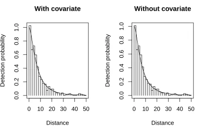
Lf. 187

The fit of the detection functions averaged over all data look similar for both models (Fig. 1) but the

188

model with the covariate is clearly better with a4AIC of 33.34. The estimate of abundance from the model

189

with the covariate is 3212 (se=261.6) and without the covariate is 3267 (se=276). For the mixed effect model

190

the estimated standard deviation (0.57) is smaller than the same quantity for the random effect model (0.67)

191

which absorbs the heterogeneity due to the missing covariate into the random effect.

192

The total abundance estimates are similar, but when abundance is estimated for each type of object

193

(with covariate: 2176 (se = 182.9) and 1036.1 (se = 155.1); without covariate: 2669 (se = 231) and 597.2

194

(se = 70.9) the importance of including the covariate becomes obvious. When using the model with the

195

covariate, the model fits tighter to the observed data (Fig. 2) in particular for the subset of the data with the

196

smaller sample size, i.e. the subset of the data with covariate value = 1. On the other hand, for the model

without the covariate predicted detection probabilities are too low for distances near zero and too high for

198

larger distances which results in an underestimate of abundance of those with covariate value 1. Likewise,

199

the estimated abundance for objects with covariate value 0 is too high.

200

4.2

Simulation comparison with hazard rate

The random scale normal detection function has two parameters and is thus more flexible than a

half-202

normal with a single parameter. The hazard rate which is often used to represent detection functions also

203

has two parameters, so a simulation comparison of the alternative two-parameter models is worthwhile.

204

We simulated data from a t-distribution with 3, 5, and 10 degrees of freedom, also from a random scale

205

half-normal (βg = -0.5; σ = 0.5) and from a hazard rate (g(x) = 1−exp(−(x/σ)−p);σ = 0.7;p = 2.5). 206

We simulated 500 replicates for each detection function with expected sample sizes of 60-90 and 130-180 by

207

varying the true abundance (N) for the scenario. The distances were generated using rejection sampling

208

with w=40 and the parameters were chosen so the largest observed distance would not exceed 20. The

209

number detected (n) and the largest observed distance (w) would vary so they are summarized as means

210

in the results (Table 1). For each data set we fit the random scale half-normal with the ADMB code from

211

theRandomScale package using Lg eq (6) andLf (see eq (13) from Appendix 1, Supporting Information) 212

and the hazard rate detection function using themrds package (Laake et al., 2013) using a transect width

213

(w) equal to the largest observed distance and twice the largest observed distance to approximate an infinite

214

width. We measured the proportion of replicates in which Akaike’s Information Criterion (AIC) was smaller

215

forLg versusLf and vice versa. Even though they should produce the same likelihood value we have found 216

that our ADMB implementation ofLf has better convergence thanLg. We also compared the proportion of 217

replicates in which AIC was smaller forLf versus the hazard rate model. For the random-scale half-normal 218

model we computed the percent relative bias (PRB=100(N−Nˆ)/N) and its simulation standard error and

219

root mean squared error (√(var( ˆN)−(N¯ˆ−N)2) expressed as a percentage of N. We also computed the

220

same quantities using the estimate from the model with the smallest AIC for each replicate. In comparing

221

abundance estimates to the true value we usedN/w which scales with the width of the transect that was

222

used.

223

As expected, the random scale half-normal and hazard rate did best when the data were generated from

224

the fitted model. In general, when generating data under a different distribution, the hazard rate tended

225

to underestimate and the random scale half-normal model tended to over-estimate abundance. However,

226

when AIC was used to select the best model, the average bias was typically less than 5% and often within

227

simulation error. The bias of the average was largest when data were generated from the hazard rate, because

the random scale half-normal tended to over-estimate the intercept and abundance because the hazard rate

229

detection function has a long tail and then flattens near x=0. For these same scenarios, the ADMB code

230

for Lg had substantial problems with convergence in comparison to Lf. In fewer than 0.2% of the 10000 231

simulations did theLgcode produce a smaller negative log-likelihood thanLf. Whenw was set to twice the 232

largest observed distance, the random scale half-normal performed better with less bias and the hazard rate

233

performed worse with more negative bias except when the hazard rate was used to generate the simulated

234

distances. In real data applications we never know the true detection function, so it is useful to have a set

235

of models to examine and use a model selection criterion like AIC.

236

5

Application to harbor porpoise data

In 2002, a small boat survey for harbor porpoise (Phocoena phocoena) was conducted in waters of the Strait

238

of Juan de Fuca and around the San Juan Islands in Washington state, USA. Three observers surveyed along

239

a set of systematically placed lines with an observer standing on the bow and at the starboard and port

240

sides. When harbor porpoise were detected, the angle from the line to the harbor porpoise was measured

241

with an angle board and the radial distance to the detection was estimated visually. Observers were trained

242

and tested in visual distance estimation but for this example, we ignore the error in distance estimation.

243

The angle and radial distance was converted to perpendicular distance. In addition to distance, the number

244

of harbor porpoise (size) was recorded for each detection.

245

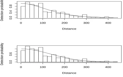
A total of 477 harbor porpoise groups were detected with group size varying from 1 to 6. We fitted a

246

model with a half-normal detection function and used group size as a covariate. We fitted a fixed effect

247

detection function with themrdspackage (Laake et al. 2013) and a mixed effects detection function with the

248

RandomScale package. Themrds package requires a finite width, so to make the AIC values equivalent we

249

setw=443.2 the largest distance for each analysis. The fit of the detection functions (Table 2) look similar

250

(Fig. 3) but the model that includes the random effect is slightly better with a4AIC of 2.6. The estimate

251

of harbor porpoise group abundance within the 886.4 meter strip is 1243 (se = 59) for the fixed effect model

252

and 1360 (se = 93) for the mixed effect model. The higher abundance estimate resulted from the slightly

253

steeper estimated detection function (Fig. 3).

254

6

Discussion

255

Incorporating a random effect in the scale of the detection function extends the covariate approach of

256

Marques and Buckland (2003) to enable modeling of additional unspecified and typically unknown sources

of heterogeneity in detection probability. This removes the need to select an arbitrary truncation width

258

which is typically needed for the CDS key-adjustment function fitting (Buckland et al., 2001). The random

259

and mixed effects modeling can be used with other detection functions such as the hazard function (Buckland

260

et al., 2001) as long as the parametrization includes a scale parameter (x/σ); although it could also be applied

261

to the shape parameter in the hazard function. The models can be easily extended to allow covariates to be

262

included for the random effects standard deviation σ. For example, heterogeneity in detection probability 263

may be enhanced or reduced as a function of weather, habitat or other covariates. We propose that a random

264

or mixed effect model of the detection function scale be adopted as one of the standard approaches for fitting

265

detection functions in distance sampling.

266

7

Ackwlowledgements

267

We thank Steve Buckland for reviewing a nearly final draft of the paper. Cornelia Oedekoven was supported

268

by a studentship jointly funded by the University of St Andrews and EP-SRC, through the National Centre

269

for Statistical Ecology (EPSRC grant EP/C522702/1). Hans Skaug thanks the Center for Stock Assessment

270

Research for facilitating his visit to University of California, Santa Cruz.

271

References

Borchers, D. and Burnham, K. (2004). Advanced Distance Sampling., chapter General formulation for

273

distance sampling. Oxford University Press, Oxford.

274

Buckland, S. T., Anderson, D. R., Burnham, K. P., Laake, J. L., Borchers, D. L., and Thomas, L. (2001).

275

Introduction to Distance Sampling. Oxford University Press.

276

Fournier, D. A., S. H. J., Ancheta, J., Ianelli, J., Magnusson, A., Maunder, M. N., Nielsen, A., and Sibert, J.

277

(2012). Ad model builder: using automatic differentiation for statistical inference of highly parameterized

278

complex nonlinear models. Optimization Methods and Software27,233–249.

279

Hedley, S. L. and Buckland, S. T. (2004). Spatial models for line transect sampling. Journal of Agricultural,

280

Biological and Environmental Statistics9,181–199.

281

Laake, J., Borchers, D., Thomas, L., Miller, D., and Bishop, J. (2013). mrds: Mark-Recapture Distance

282

Sampling. R package version 2.1.4.

283

Marques, F. F. C. and Buckland, S. T. (2003). Incorporating covariates into standard line transect analyses.

284

Marques, T. A., Buckland, S. T., Borchers, D. L., Tosh, D., and McDonald, R. A. (2010). Point transect

286

sampling along linear features. Biometricspage no.

287

Marques, T. A., Thomas, L., Fancy, S. G., and Buckland, S. T. (2007). Improving estimates of bird densities

288

using multiple covariate distance sampling. The Auk124,1229–1243.

289

Miller, D. L. and Thomas, L. Mixture models for distance sampling detection functions. Unpublished

290

manuscript.

291

Pledger (2000). Unified maximum likelihood estimates for closed capture-recapture models using mixtures.

292

Biometrics56,434–442.

Table 1: Percent relative bias (PRB) and root mean square error (RMSE) as proportion of true abundance for random scale half-normal and hazard rate detection function models for distances generated from t-distribution, random scale half-normal and hazard rate detection functions. Each value is the summary for 500 replicate simulations; ¯wand ¯nare the mean truncation distance and mean sample size. The subscripts F, G and HR refer to

Lf, Lg and the hazard rate. AVG subscript represents the values in which the estimate was generated from the model that had the lowest AIC for each replicate. Data were generated from a t-distribution with listed degrees of freedom (t(df)), a random scale half-normal (hn) withβg = -0.5 and

σ= 0.5 , and a hazard rate (hr;g(x) = 1−exp(−(x/σ)−p withσ= 0.7 andp= 2.5).

Function w¯ n¯ P RBF P RBHR P RBAV G se(P RBAV G) AICF < AICHR AICF < AICG AICG< AICF RM SEF RM SEHR RM SEAV G

t(df=3) 8.80 136.46 8.67 -9.80 -2.25 0.84 0.39 0.14 0.00 16.67 18.61 18.87

17.23 136.46 6.23 -13.01 -0.97 0.80 0.63 0.16 0.00 17.97 17.02 17.81

t(df=5) 5.23 132.30 7.46 -7.92 -0.86 0.77 0.46 0.06 0.00 15.73 16.89 17.13

10.47 132.30 4.04 -12.50 -0.21 0.68 0.76 0.09 0.00 17.34 14.62 15.29

t(df=10) 3.70 128.09 4.88 -7.98 -2.11 0.68 0.46 0.08 0.00 14.97 14.47 15.26

7.41 128.09 1.54 -13.58 -1.19 0.60 0.84 0.07 0.00 17.82 12.74 13.57

t(df=3) 6.86 68.18 15.08 -3.78 2.11 1.34 0.29 0.10 0.00 23.95 33.18 30.01

13.63 68.18 8.84 -10.11 0.43 1.13 0.57 0.10 0.00 21.95 26.57 25.24

t(df=5) 4.32 66.16 11.24 -3.64 1.74 1.14 0.34 0.06 0.01 22.19 27.56 25.66

8.64 66.16 4.51 -11.48 -0.59 1.01 0.70 0.11 0.01 21.69 22.20 22.59

t(df=10) 3.24 63.65 10.92 -1.82 2.37 2.55 0.34 0.03 0.00 23.77 27.04 25.58

6.48 63.65 3.62 -12.01 0.00 2.12 0.77 0.08 0.03 21.33 20.14 21.23

hn 4.52 172.60 3.33 -12.28 -2.51 0.69 0.62 0.06 0.00 17.21 14.27 15.68

9.03 172.60 0.02 -16.62 -2.03 0.63 0.89 0.12 0.00 20.11 13.43 14.32

hn 3.79 86.50 8.28 -7.32 -0.80 1.02 0.39 0.04 0.00 20.00 23.58 22.85

7.59 86.50 2.09 -13.69 -1.41 0.91 0.79 0.07 0.00 21.57 19.87 20.47

hz 15.67 183.22 20.22 2.87 3.11 1.09 0.01 0.80 0.00 10.96 28.48 11.34

28.48 183.22 19.44 1.94 4.28 1.30 0.09 0.82 0.00 10.68 27.64 13.72

hz 12.57 91.44 24.97 4.01 5.32 0.87 0.05 0.56 0.00 17.98 35.94 20.17

22.68 91.44 23.32 2.40 5.76 0.90 0.14 0.55 0.00 17.12 34.27 20.93

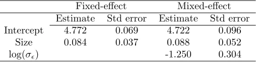
Table 2: Parameter estimates, standard errors for fixed (AIC=5375.7) and mixed effect (AIC=5373.1) models fitted to harbor porpoise vessel survey data.

Fixed-effect Mixed-effect Estimate Std error Estimate Std error Intercept 4.772 0.069 4.722 0.096

Size 0.084 0.037 0.088 0.052

0

10 20 30 40 50

0.0

0.2

0.4

0.6

0.8

1.0

With covariate

Distance

Detection probability

0

10 20 30 40 50

0.0

0.2

0.4

0.6

0.8

1.0

Without covariate

Distance

Detection probability

0 10 20 30 40 50

0.0

1.0

Model with covariate

covariate value=0

Distance

Detection probability 0 10 20 30 40 50

0.0

0.8

Model with covariate

covariate value=1

Distance

Detection probability

0 10 20 30 40 50

0.0

0.8

Model without covariate

covariate value=0

Distance

Detection probability 0 10 20 30 40 50

0.0

1.0

Model without covariate

covariate value=1

Distance

Detection probability

0 100 200 300 400

0.0

0.4

0.8

Distance

Detection probability

Distance

Detection probability

0 100 200 300 400

0.0

0.6

Supporting Information

Additional Supporting Information may be found in the online version of this article:

295

296

Appendix S1: Comparison between two likelihood formulations for the random scale detection function

297