Power Network Asymmetrical Faults Analysis Using Instantaneous Symmetrical Components

doi:10.4236/jemaa.2009.14031 Published Online December 2009 (http://www.SciRP.org/journal/jemaa)

Power Network Asymmetrical Faults Analysis

Using Instantaneous Symmetrical Components

S. LEVA

Department of Energy, Politecnico di Milano, Via La Masa, Milano, Italy. Email: [email protected]

Received October 9th_{, 2009; revised November 3}rd_{, 2009; accepted November 10}th_{, 2009.}

ABSTRACT

Although the application of Symmetrical Components to time-dependent variables was introduced by Lyon in 1954, for many years its application was essentially restricted to electric machines. Recently, thanks to its advantages, the Lyon transformation is also applied to power network calculation. In this paper, time-dependent symmetrical components are used to study the dynamic analysis of asymmetrical faults in a power system. The Lyon approach allows the calculation of the maximum values of overvoltages and overcurrents under transient conditions and to study network under non-sinusoidal conditions. Finally, some examples with longitudinal asymmetrical faults are illustrated.

Keywords: Power System Fault Analysis, Asymmetrical Faults, Symmetrical Components, Lyon Transformation

1. Introduction

The general Fortescue Symmetrical Components Transf- ormation (SCT) [1,2] is formalized in phasor terms. It can only be used to study steady-state conditions that follow the fault transient condition. The maximum values of overvoltages and overcurrents can only be calculated in an approximate way by means of corrective factors [3].

Recently, the space-vector transformation – used in machine vector control – has been applied to power sys-tem analysis, too [4,5]. Currently, network theory and complex transformation suggest that the study of asym-metrical faults can be carried out by means of instanta-neous sequence components [6–9].

As a matter of fact, by using the same topological ap-proach of the SCT, it is possible to directly analyze the faulty network by differential equations that represent the faults not only in steady-state conditions but also under transient conditions.

As shown by W. Lyon [10,11], the formal aspects of the procedure can be summarized by the following points:

1) the phasors that represent phase- and sequence- variables, are substituted by time-dependent functions, so that the concept of Fortescue sequences can be general-ized to the concept of instantaneous sequences;

2) the Fortescue matrix [ ]S remains the same, and hence the method confirms the SCT topological and mo-dal-analysis approach [11,12];

3) the phasor operator j is replaced by the derivative operator p d dt / . Under this assumption, differential analysis is required and depends on the Cauchy initial conditions; and

4) the sequence impedances are converted form ( )

Z j to generalized form z(p), maintaining the same circuital and topological meaning.

This time-domain analysis is characterized by three fundamental features. The first is an applicative one, which regards the ability to calculate - without the use of corrective coefficients – the maximum values of overvol- tages and overcurrents during the transient conditions. This is very important for circuit-breaker sizing and the evaluation of the electro-dynamic force between busbars and in transformer windings. The second characteristic concerns the possibility of studying not only sinusoidal, but also non sinusoidal sources. The last characteristic regards the formal and methodological aspects introduc- ed by using the Lyon approach. By means of the Lyon approach, the procedures of dynamic analysis of the network can be unified. In addition, by substituting the SCT with the Lyon approach, fault analysis can be car-ried out by using the state equations that can be inte-grated by classic procedures based on system analysis and the graph approach. The state-equation solutions, can be expressed in literal form by means of analytical for-mulations if the network is linear and time-invariant.

ons, steady-state phasors and well-known sequence net-works are given and illustrated through the use of an example with an asymmetrical fault in [6]. The use of dynamic phasors together with space-vectors – incorpor- ating the frequency information – in power system analy-sis is presented in [7] and [8]. To complete these studies in the following, a systematic analysis of the asymmetri-cal faults is developed and deeper investigated both from the theoretical and applicative points of view, giving some important observations that are very useful to achieve the numerical analysis and to better understand the results obtained by using industrial software pack-ages.

The Lyon approach to study transient and steady-state conditions of transversal and longitudinal faults is de-veloped in terms of the following scheme: in Section 2, the Lyon Transformation is recalled and its link with SCT is investigated. In Section 3, the application of the Lyon method to the study of asymmetric transversal and longitudinal faults is formalized and some remarks con-cerning the connection conditions and the use of state-equation approach are put in evidence; furthermore the equivalent model of each fault is calculated. Finally, in Section 4, some numerical examples emphasize the validity of the proposed approach by comparing the ob-tained results with those derived by the SCT method.

2. The Lyon Transformation

Considering an arbitrary time function three-phase set {wa(t), wb(t), wc(t)}, the Lyon transformation gives the

following decomposition (where  exp( 2 / 3)j  ):

 

 

 

 

 

 

 

 

 

2

2

1 1 1

1 1 3

1

a o

b

c

w t w t w t

w t w t S w t

w t w t w t

 

  _ 

       

 _  _ _{ } 

 

       

  _ _    

     

o



(1)

from which it is possible to observe that the matrix

 

S is formally the same for both SCT and Lyon transformation. On the other hand, the functions sub-jected to the Lyon Transformation assume a generic time trend.

Taking into account that

 

1

 

T

S  _ S

then:

 

 

 

 

 

 

0

2

2

1 1 1

1 ₁ 3 ₁





    

 _  _

    

  _ _ 

  

a

b

c

w t w t

w t w t

w t w t

 

 

   

(2)

Therefore, it is possible to define, starting from a generic three-phase set in time domain, the instanta-neous symmetric components named, respectively.

zero-, positive-, and negative-sequences. The zero- sequence component w t₀

 

is always real. The nega-tive-sequence component w t

 

is the complex

con-jugate of the positive sequence component w t_

 

. Analyzing Equations (1) and (2) we can see that the Lyon method suggests, time by time and referring to a generic waveform in time domain, the same topologi- cal procedures just used with SCT. Moreover, the Lyon transformation, applied to a generic sinusoidal three-phase set, gives the same results provided by the SCT.

Furthermore, the positive Lyon vector satisfies the following identity:

 

₂

 

₂

 

j t  dq

w t  w t  w t e  (3)

and hence it is linked to both Clarke w( )t and Park

( )

dq

w t vectors, except for a trivial proportionality factor.

The Lyon transformation, in the context of the modal analysis procedure of the actual three-phase theory, unifies all transformations normally used for dynamic analysis of power networks. In particular – as

( ) ( )

w t w t

   – the real and complex pair of time

functions w t₀( ) and w t_( ) is totally representative of the generic three-phase set of real time functions {wa(t), wb(t), wc(t)}.

The instantaneous power, in terms of the Lyon com-ponent, is [13]:

 

 

 

 

 

0 0

p abc t abc

t t

t v t i t

v_ t S S i_ t

   

_{  } _

  

_{ }    _{   } _ _ (4)

3. Lyon Approach to the Study of

Asymmetrical Faults

Lyon decomposition in instantaneous sequence compon- ents allows the use of the SCT topological procedures for studying asymmetrical faults that can occur in a power network, by using the Substitution Theorem and the Su-perposition Principle as in SCT [12-14].

Some fundamental remarks about the application to the fault analysis of the Lyon method rather than the SCT are discussed in the following sections.

3.1 Fault Equivalent Networks

In aggreement with Fortescue SCT, the instantaneous sequence networks connection corresponding to the analysed fault configuration starting from the phase cir-cult fault conditions calculation is necessary.

is not possible using Fortescue analysis. Consequently, it is important to verify that the connection conditions ob-tained starting from the real conditions are coherent with respect to the definition of an instantaneous sequence components given by (2).

As an example, in the case of a single-phase-to-ground fault, the following relationa are obtained:

 

 

 

 

 

 

   

0

0 3 f p 0

i t i t i t

v t v t v t z i t

 

 

 



 _{    }

 (5)

where zf(p) is the fault impedance. The first line of (5)

shows that the two current Lyon vectors, which are con-jugates, have to be real in order to obtain the zero-sequence current. Moreover, from the second line of (5):

 

 

 

   

 





   

0 0

0

3

2 Re 3

f

f

v t v t v t z p i t v t z p i t

 



     

      (6)

Equation (6) confirms that v0(t) is a real time function, too. Similar observations can be applied to the other fault conditions.

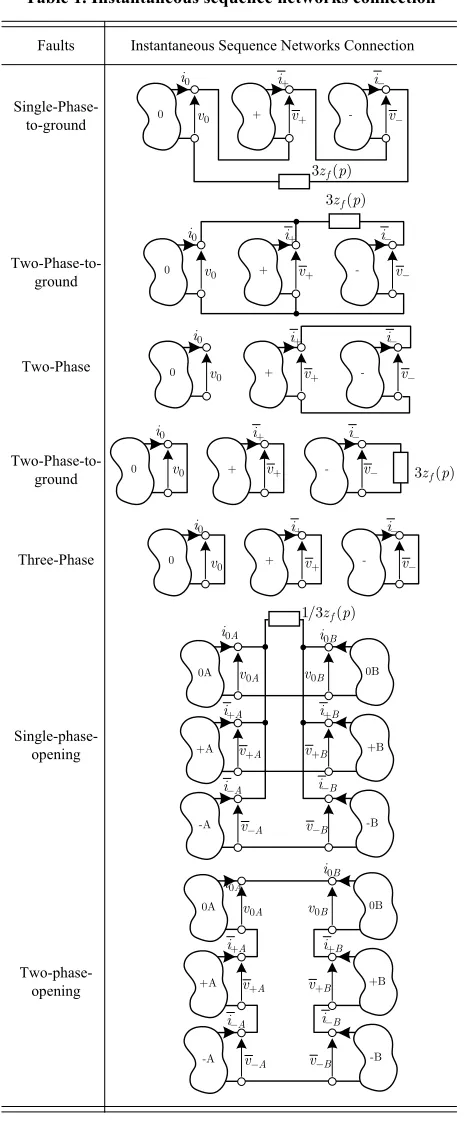
The equivalent sequence networks for each fault type are reported in Table 1. Examination of Table 1 reveals that the instantaneous sequence networks connections for the different fault types are equal to that obtained by us-ing Fortescue SCT. This is in agreement with the fact that the Lyon and Fortescue transformations use the same transformation matrix

 

S . In the time-differential do-main it is possible to use the same phasor expression only by substituting the j factor with the p operator. The complex impedance (Z j) becomes the real imp- edance z p

 

[15]. Nevertheless, the Lyon transformati- on is of greater generality than the Fortescue transforma- ation: Lyon acts on the time domain, not only in the phasor domain. The SCT can be considered as a particu-lar case of the more general instantaneous sequence components approach.

The results shown in Table 1 and the listed remarks complete the study presented in [6] and [8] analyzing in a systematic way all the asymmetrical faults and presenting the equivalent models of the faults.

Furthermore, Table 1 data together with the aforemen- tioned remarks are very important not only from the theoretical point of view, but, as a matter of fact, these results can be very useful also to the power system ana-lyst to verify the results obtained by using industrial software packages.

3.2 The State-Matrix Approach

The Lyon dynamic analysis of asymmetrical faults can be performed by using the state-matrix approach. It is divided into three distinct stages. In the first step the

[image:3.595.308.541.161.722.2]

power system is represented by the appropriate equival- ent sequence networks. The corresponding Lyon state variables (voltages across the capacitors and current flowing in the inductors) are deduced and collected in the Lyon state-vector [x].

Table 1. Instantaneous sequence networks connection

0 +

-0 +

-0 +

-0 v 0 i

v+ i+

v -i

-3 ( )z pf

0 v 0 i

v+

i+

v

-i

-0 v 0 i

v+

i+

v

-i

-3 ( )z pf

3 ( )z pf

0 _v0 +

-0 i

v+

i+

v

-i

-0A 0B

+A +B

-A -B

0A

v

A

v+

A

v

-A

i+

A

i -0A

i

B

i+

B

i -0B

i

0B

v

B

v+

B

v

-1/3 ( )z pf

0A 0B

+A +B

-A -B

0A

v

A

v+

A

v

-A

i+

A

i -0A

i

B

i+

B

i -0B

i

0B

v

B

v+

B

v

-0 v₀ +

-0 i

v+

i+

v

-i -Faults Instantaneous Sequence Networks Connection

Single-Phase-to-ground

Two-Phase-to-ground

Two-Phase

Two-Phase-to-ground

Three-Phase

Single-phase-opening

In the second step, by means of the system and topo-logical procedures of network theory [14], the mathe-matical model of the dynamics of the fault is deduced. Assuming the constitutive relations linear and time- in-variant, it is a priori formalized as:

         

         

d _{x A x B u} dt

y C x D u

 _{   }

 

 _{   }



(7)

where the input [u(t)] and the network variables [y(t)] Lyon vectors are present. The [y(t)] vector can be re-garded as the output of the system.

The solution of (7) is well-known and can be obtained in closed form. In fact, knowing the initial values of state variables (at time t=t0), it is possible to assume the

fol-lowing expression [14-16]:

 

   

_

_

   

_{  }

_

0

0

( ) o ( ) ( )

t

A t t A t

t

x t e    x t 

_

e    B  u  d (8)

where the first term represents the solution with zero inputs and the second term represents the zero state solu-tion. This last term is calculated considering the general sources [u(t)] expressed in the time domain. In the par-ticular case of sinusoidal inputs, it corresponds to the results also obtained in the phasor domain with SCT when the transient is finished.

The dynamics of the fault depends on the state fault matrix [A], and its elements depend on the sequence pa-rameters related to the type of fault that occurs in the considered power network, and on the initial conditions [x(t0)] analyzed in the following paragraph. The

eigen-values of the fault matrix [A] depend on the type of fault and characterize the dynamic of the power system during the fault.

Finally, in the third stage of the study, the network variables [y(t)] are calculated from the second line of (7). The network variables are usually Lyon voltages [v(t)] and currents [i(t)] expressed in the time domain. Equa-tion (1) allows the derivaEqua-tion of the fault dynamics ex-pressed in phase quantities.

Regarding the role of initial conditions, the zero-state network represents the simpler case for a dynamic analy-sis. In fact, in this case, the inductances and the capaci-tances are in zero-state conditions.

If the fault occurs in a non-zero state network, the state variables assume a non-zero initial state [x(t0)]=[x0]; in

this case, the voltage vC(t) across a capacitor C and the

current iL(t) flowing in an inductor L result to be:

 

 

 

 

0

0

0

0

1

1

t

C C C

t t

L L L

t

v t V i d

C

i t I v d

L

 

 



  

  

 _{  }

 





(9)

0

C

V

1

Cp

0

L

I Lp '_{( )}

C

v t

( ) C

i t

( ) L

v t

( ) L

i t

(a) (b)

1

Cp

Lp

( ) C

v t v tL( )

( ) C

i t

( )0 0

C C

v - ₌V i_L( )0- ₌I_L0

( ) L

i t

( ) C

v t

'_{( )}

L

[image:4.595.331.518.88.240.2]

i t

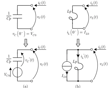
Figure 1. Method that can be used to include the initial condition of the state variables in the proposed approach; case of the capacitance (a) and of the inductance (b). It is represented in the general case, and it is valid for all the instantaneous sequence (+, − and 0)

The reactive elements can be considered in the dy-namic analysis with an initial zero state condition simply by linking them with a generator that represents the ini-tial conditions (see Figure 1).

In this way, the capacitor must be connected in series with a voltage generator (equal to VC0) and the inductor

must be connected in parallel with a current generator (equal to IL0). The new state variables are represented by

the voltage '

 

C

v t across the capacitor C and the current

 

' L

i t flowing in the inductor L, respectively. Equation (8) becomes:





   

_{  }

_

0

'

'( ) ' '( )

t

A t

t

x t _ e   _ B _ u  _d



(10)

where [A’], [B’] and [u’(t)] are calculated considering the new network.

This method is particularly important and useful in the analysis of power networks where some inductances (capacitors) are connected in series (in parallel) with dif-ferent initial conditions.

4. Applicative Case

The Lyon approach to studying power system faults pre-sented in this paper is now applied to investigate the cur-rent fault in two diffecur-rent power systems. The first power system is represented by a classic three-phase line consi- dered by other Author [15]. This example can be considered to validate the Lyon method. The second ex- ample regards the fault analysis in a real network used in Italy.

4.1 Transient Fault Analysis of a Basic Power System

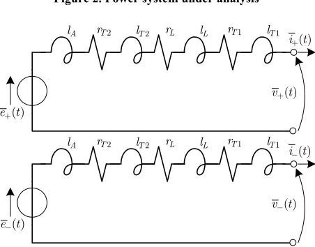
phase line L, and a transformer T1. The system has no load when the fault occurs. No information about the grounding connection of the neutral conductor of the generator and transformers is reported in [15], conseque- ntly only the three-phase and two-phase faults are ana-lyzed because they are independent to the grounding connection.

The corresponding positive- and negative- instantane- ous sequence networks are reported in Figure 3; the quantities indicated are deducted from the data reported in Figure 2 [5]. The analysis of the previously indicated fault types does not require the zero-sequence instantane- ous network.

The Lyon quantities w t₀

 

, w t w t_( ), ( )_ are be ex-pressed as follows:

 

 

 

0

0 0

1 ₂

0

0

1

2 j

w

w S e We

w





 

 

 



  _{   }

 _{  } _{ } _ _

 _{    }

 

  _{ }



  

(11)

Three-phase fault analysis: in this case the positive- and negative- instantaneous sequence networks are short-circuited at the point of the fault.

where 0 represents the a phase angle (respect to the

real axis) in which the fault occurs. The corresponding state equations are:

60 MVA 10.5 kV 12 % G nG d

A V x

   

40 MVA 10.5/63 kV

10 % 0.4 % T

k r

A

u u



 

60 kV 22 km

0.4 /km 0.255 /km nL

L L

V L x r

 

 

 

12 MVA 60/10.5 kV

8 % 0.65 % T

k r

A

u u



 

[image:5.595.67.282.419.493.2]

A T2 L T1

Figure 2. Power system under analysis

( ) e t₊

( ) i t₊

( ) v t+ A

l rT2 lT2 rL lL rT1 lT1

( ) e t

-( ) i t

-( ) v t

-A

l rT2 lT2 rL lL rT1 lT1

Figure 3. Positive- and negative- instantaneous sequence net works for the analysis of three-phase and two-phase faults

  

   



 

  

   



 

2 1 2 1

2 1 2 1

T L T A T L T

T L T A T L T

e t r r r i t l l l l pi t e t r r r i t l l l l pi t

 

 

        

 

        







(12) where r and l are the pu resistances and impedances re-spectively.

The line phase currents calculated during the fault are shown in Figure 4. Figure 4 shows the transient move-ment considering φ0=0 and φ0=π/4 respectively, where φ0

represents the phase angle a in the fault instant.

The steady state (sinusoidal condition) values match those calculated by using STC. The maximum value in the steady state condition of the phase fault currents is equal to 0.5208 pu. Under transient conditions the phase currents calculated by using Lyon or STC are instead different. The maximum value reached by the currents during the entire transient depends on φ0. In fact, during

the first period of the transient with φ0 = 0, two phase

currents reach the value of 0.8 pu, while withφ0 = π/4 the

phase b reaches 0.83 pu.

In Figure 5, the vector i t

 

is depicted in the comp-

lex plane. By using a complex vector and its polar repre-sentation the vector magnitude can easily be depicted [5]. The initial magnitudes correspond to the initial condition equal to zero. During the first fault transient instant the current reaches its instantaneous maximum value. At the end of the transient, under steady-state and symmetric condition, the current i t

 

describe a perfect circle.

Two-phase fault analysis: in this case the instantaneo- us sequence networks are connected in parallel. The cor-responding state equation is:

 

  

  



2 12



 

1

2 2

T L T

A T L T

e t e t r r r i t l l l l pi t

  



    

[image:5.595.60.286.507.684.2]

     (13)

Figure 6 shows the line phase currents during the en-tire transient fault calculated with ₀ 0 and

0 4

  respectively. The maximum value of the currents at the end of the transient (sinusoidal steady-state condi-tion) is 0.451 pu equal to that calculated by using SCT.

Whit φ0 = 0, the b and c phase fault currents reach,

during the first period, a maximum value equal to 0.7317 pu. With φ0 = π/4, the maximum value is 0.64 pu.

In this case the real part of the current vector i t

 

is

approximately zero. In accordance with (2), the vector only moves along the imaginary axis of the complex plane starting from 0.

4.2 Transient Fault Analysis of an Existing Power System

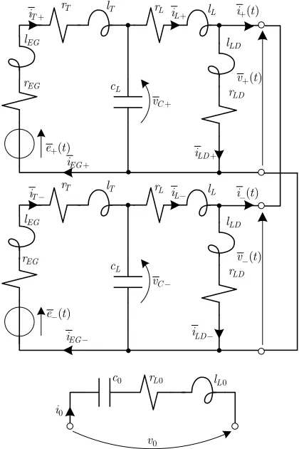
7). The network under analysis is constituted by a high voltage external grid EG, a transformer T, a line L, and a medium voltage load LD. The faults occur on the me-dium voltage busbars.

(a)

[image:6.595.322.523.86.428.2]

(b)

Figure. 4. Three-phase fault: phase currents transient with (a) φ0=0 and (b) φ0=π/4

-0.6 -0.4 -0.2 0 0.2 0.4 -0.4

-0.3 -0.2 -0.1 0 0.1 0.2 0.3 0.4 0.5 0.6

Re

Im _{i t}

_{ }

[image:6.595.70.276.142.471.2]



Figure 5. Three-phase fault: Lyon time vector i t

 

with

0 4

 

(a)

[image:6.595.334.511.470.529.2]

(b)

Figure 1. Two phase fault: phase currents transient with (a)

φ0 = 0 and (b) φ0 = π/4

EG T

10 km

15 kV LD L

132 kV

Figure 7. One line diagram

To set up the network circuit, the line L is represented by a “Γ” cell, while the transverse parameters of the tran-sformer T are neglected. Furthermore, the transformer is shell core type, which means that the zero-sequence flux component flows in the low reluctance core. Consquently, the zero-sequence impedance is very high. The load is represented by a simple set of impedances. The neutral condition of the external high voltage grid EG is-grounded, while the medium voltage side is not grounded. The network data are reported in Table 2.

[image:6.595.66.280.514.676.2]

[image:7.595.59.288.89.626.2]

Table 2. Numerical parameters of the network in Figure 7

Elements Data

Nominal voltage V_n132 kV

Short-circuit current (HV side) IkHV 3 12 kA

EG

Short-circuit power factor cos _k 0.1

Connection Y0y

Nominal power An25 MVA

Nominal voltage (HV side) V_nHV132 kV Nominal voltage (MV side) VnMV 15 kV Short-circuit voltage v_sc15 5. %

Short-circuit power P_sc35 kW

No-load current i01%

Tran

sfo

rmer

No-load power P026 kW

Nominal voltage V_n15 kV

Length L10 km

Resistance r10.226Ω/km

Inductance x10.35Ω/km

Capacitance c19.65 nF/km

Zero-sequence resistance r00.371Ω/km Zero-sequence inductance x01.536Ω/km

Lin

e

Zero-sequence capacitance c04.51 nF/km

Nominal voltage Vn15 kV

Active power P_c9 MW

Lo

ad

Reactive power Qc3.5 MVAr

, ( ) e_{+ -}t

, ( )

i_{+ -}t

, ( )

v_{+ -}t

EG

r

EG

l

T

r lT

L

c

,

C

v ₊

-L

r l_L rLD lLD

,

LD

i ₊

-,

EG

i ₊

-,

T

i₊

-,

L

i₊

-0

v

0 i

0

c rL0 lL0

Figure 8. Positive-, negative-, and zero-sequence instantane- neous sequence networks for the transversal fault analysis of the network depicted in Figure 7

network is composed only by the line zero-sequence pa-rameters.

The computation of the initial condition is performed

calculated starting from the data reported in Table 2. Based on the hypothesis about the type of load and the neutral point connection, the instantaneous zero-sequence

fault occurs. The state quantities result: considering the network under the sinusoidal condition before the

0.165 0.0921 pu 0.1649 0.0923 pu

EG _T

L LD

I I j

I I j

  

  

0.5619 0.02685 pu

C

V  j

(14)

Single-phase-to-ground fault. The seque

are connected in series. The fault does not change the line current values very much: no more than a very small tra

transient - sinusoidal an

zero-instantaneous sequence network is open nce networks

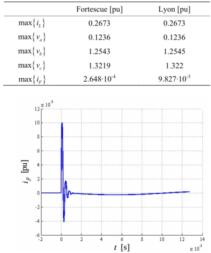
nsient in the first instants of the fault transient is pre-sent. The fault current (see Figure 9) instead presents in the first instant high frequency oscillations superimposed to the fundamental network frequency (50 Hz). These oscillations with high amplitude decay very rapidly. Nevertheless, the fault current is very low because the network is not grounded: the unique path to the ground is represented by the line capacitors.

Table 3 shows the maximum value of the line currents and voltages calculate by using Fortescue SCT and Lyon ISCT, which are – at the end of the

d equal.

[image:7.595.57.288.100.630.2]

Two-phase fault. In this case, the positive- and nega-tive-instantaneous sequence networks are connected in parallel, the

Table 3. Comparison between maximum value evaluated by SCT and ISCT

Fortescue [pu] Lyon [pu]

 

max iL 0.2673 0.2673

 

max va 0.1236 0.1236

 

max vb 1.2543 1.2545

 

max v_c 1.3219 1.322

 

max i_F 2.648·10-4 9._827·10-3

[image:7.595.316.527.451.704.2]

as shown in Figure 10. Figure 11 shows the line current movement during the fault transient calculated consider-ing φ0= 0. A high peak in the considered quantities can

be observed. In particular, the phases b and c show a peak in the first instants equal to 1.5141 pu and 1.3826

0 v 0

i

0

c rL0 lL0

( )

e t+

( )

i t+

( )

v t+

EG

r

EG

l

T

r l_T

L

c

C

v +

L

r l_L

LD

r

LD

l

LD+ i

EG

i +

T

i + iL+

( )

e t

-EG

r

L

c

EG

l

T

r l_T

C

v

-L

r l_L

EG

i

-T

i - iL- i t-( )

( )

v t

-LD

r

LD

l

LD

i

-Figure. 10. Instantaneous sequence networks connection for the analysis of two-phase fault

-1.5 -1 -0.5 0 0.5 1 1.5

-1 -0.5 0 0.5 1

Re

Im

  L

i t

[image:8.595.311.514.90.244.2] [image:8.595.67.277.152.467.2]

 

L i_ t Figure 12. Two phase fault: Lyon time vector wit

Table 4. Current maximum values as a function of φ0 h

φ0 = 18°   0

  max



iLa b c, ,  t



pu  max



iLa b c, ,  t



/ILMax

-90 1.2859 4.8109

-80 1.3126 4.9108

-60 1.372 5.1331

-40 1.4323 5.3587

-20 1.4841 5.5525

-10 1.5027 5.6221

0 1.5141 5.6647

10 1.5168 5.6748

20 1.5094 5.6471

40 1.4577 5.4537

60 1.3505 5.0526

80 1.2619 4.7212

Table 5. Current maximum value as a function of φ0

 

0

  max



i_{La b c, ,}  t



pu  max



i_{La b c, ,} t



/I_LMax

-80 1.6685 1.2429

-60 1.6365 1.2191

-40 1.6515 1.2303

-20 1.6685 1.2429

-10 1.6597 1.2364

0 1.6365 1.2191

10 1.6290 1.2135

30 1.6654 1.2406

50 1.6597 1.2364

70

90 1.6654 1.6290 1.2135 1.2406

pu respectively: th values cann lculated by usi Fortescue .

In t kind of fau ne currents ass e values in the nstant ult. The max alue de- pends on the phase angle φ. I Table IV the maximum val-ues

ese peak ot be ca ng analysis

his lt, the li ume larg

first i of the fa imum v

0

reached by the line phase currents ( n

 



max i _{, ,} t



and the ratio between this value and the m under the pre-fault sinusoidal condition (

La b c )

[image:8.595.312.534.298.444.2]

aximum value 2

Figure 11. Two phase fault: line phase currents transient calculated with φ0=0

LMax L

[image:8.595.310.534.462.594.2] [image:8.595.61.283.518.690.2]

maximum value is reached for φ0=18°: the ratio

(max



La b c, ,

 

t



/I

Fig 12 shows

LMax) is

i close to 5.70.

vector

ure the Lyon iL

 

e

com-rst fault transient instant the ous maximu . At the eady-state but metric

t in th plex plane. During

curre s its instantane end o he transien

condition, the curren the fi

nt reache m value

f t t, in st t

in asym

 

L

ha

i t describes an ellipse.

an ungrounded network that

lt case, Table V The two-phase-to-ground fault analysis leads to very similar results. It depends on

s a very high neutral to ground impedance.

Three-phase fault. In this case the instantaneous se-quence networks are short-circuited at the point where the fault occurs. As for the two-phase fau

shows the maximum values reached by the line phase currents (max



i_{La b c, ,}

 

t



) and the ratio between this value and the maximum value under the pre-fault sinu-soidal condition (ILMax  2IL ) calculated for

differ-ent phase angles ₀ . In this case, the peak value achieved in the first instants is 1.24 time he maximum value of the current in the final steady-state condition.

5. Conclusions

The use, in the time-doma n analysis, of Lyon transform- ation of asymmetric transversal faults is shown.

s t

i

st.

na

character

y employed for fault analysis, ca rticular case of the more gene

[2]

port D’Energie Electrique, Dunod, ” Paris, 1966.

lculations,”

[7] A. M. Stankovi sis of

asymmetri-cal faults in p namic phasors,”

anced and

in

cas,

. Williams, J. J. DiStefano, Schaum's, The

proposed approach allows the derivation of the Lyon state model of the faulted network and of the transient and steady state voltages and currents of intere

Thanks to the Lyon approach, the peak values reached in the first instants of the fault by the network voltages and currents can be calculated. Furthermore, the complex vectors allow the use of the state equations approach to perform th mic analysis and provide sim-ple relations to steady-state phasors and their rms values. The Lyon approach can also be used for derivation of equivalent circuits ize the different faults and – thanks to the state-matrix approach – its eigenval-ues. These information can be very useful to the power system analysts before starting their analysis by software package simulations.

e network dy

that

nall pa The SCT, traditio

be considered as a ral n

three-wire, three-phase systems,” L’Energia Elettrica, Vol. 81, No. 5–6, pp. 51–56, 2004. [14] W. Lyon, “Application of the method of symmetrical

compo-nents,” Mc Graw-Hill Book Company, New York, 1937. instantaneous sequence components approach proposed

by Lyon.

Finally, the examples here presented confirm that the use of time-dependent symmetrical component in net-work calculations has several advantages with respect to the SCT and simulation software: the Lyon transforma-tion allows transient calculatransforma-tions; the simple relatransforma-tion with their steady-state phasors facilitates the interpreta-tion of the results by the well-known steady-state phasor theory and by using complex plane diagrams.

Finally, it is important to underline that network com- ponent data are usually available in these coordinates.

REFERENCES

[1] C. L. Fortescue, “Method of symmetrical coordinates applied to the solution of polyphase networks,” AIEE Trans., pt. II, Vol. 37, pp. 1027–1140, 1918.

C. F. Wagner and R. D. Evans, “Symmetrical components,” Mc-Graw-Hill Book Company, Inc., New York, 1933. [3] H. Edelman, “ThEorie Et Calcul Des REseaux De

Trans

[4] L. O. Chua, C. A. Desoer, and E. S. Ku, “Linear and non linear circuits,” McGraw-Hill Inc, New York, 1994. [5] S. Leva and A. P. Morando, “Analysis of physically

symmetrical lossy three-phase transmission lines in term of space vectors,” IEEE Transactions on Power Delivery, Vol. 21, No. 2, pp. 873–882, 2006.

[6] G. C. Paap, “Symmetrical components in the time domain and their applications to power networks ca

IEEE Transactions on Power Systems, Vol. 15, No. 2, 522–528, 2000.

ć and T. Aydin, “Analy ower systems using dy

IEEE Trans. on Power Systems, Vol. 15, No. 3, pp. 1062–1068, 2000.

[8] S. Huang, R. Song, and X. Zhou, “Analysis of bal

unbalanced faults in power systems using dynamic phasors,” IEEE Proceedings of International Conference on Power Systems Technology, Vol. 3, pp. 1550–1557. 2002. [9] J. M. Aller, A. Bueno, M. I. Giménez, V. M. Guzmán, T.

Pagà, and J. A. Restrepo, “Space vectors applications power systems,” IEEE proceedings of Third International Conference on Devices, Circuits and Systems, Cara pp. 78/1–78/6, 2000.

[10] W. Lyon, “Transient analysis of alternating-current ma-chinery,” J. Wiley & Sons, New York, 1954.

G. J. Retter, “Matrix and space-phas

[11] or theory of electrical

machines,” Akadémiai Kiadó, Budapest, 1987.

[12] A. Gandelli, S. Leva, and A. P. Morando, “Topological considerations on the symmetrical components transfor-mation,” IEEE Transactions on Circuits and Systems, Vol. 47, No. 8, pp. 1202–1211, 2000.

[13] A. Ferrero, S. Leva, A. P. Morando, and A systematic, “Mathematically and physically sound approach to the energy balance in

[15] S. Leva, A. P. Morando, and D. Zaninelli, “Evaluation of line voltage drop in presence of unbalance, harmonics and interharmonics: Theory and applications,” IEEE Transac-tions on Power Delivery, Vol. 20, No. 1, pp. 390–396, 2005. [16] A. J. Stubberud and I. J

“Outline of feedback and control systems,” Schaum's, McGraw-Hill, New York (USA), 2nd _{Edition. 1990.}