The structure of galaxies : the division of stellar mass by morphological type and structural component

(1)

STELLAR MASS BY MORPHOLOGICAL TYPE AND

STRUCTURAL COMPONENT

Lee Steven Kelvin

A Thesis Submitted for the Degree of PhD

at the

University of St Andrews

2013

Full metadata for this item is available in

Research@StAndrews:FullText

at:

http://research-repository.st-andrews.ac.uk/

Please use this identifier to cite or link to this item:

http://hdl.handle.net/10023/3689

(2)

The Structure of Galaxies

The Division of Stellar Mass by Morphological Type and Structural Component

by

Lee Steven Kelvin

Submitted for the degree of Doctor of Philosophy in Astrophysics

(3)

(4)

Declaration

I, Lee Steven Kelvin, hereby certify that this thesis, which is approximately 60,000 words in length, has been written by me, that it is the record of work carried out by me and that it has not been submitted in any previous application for a higher degree.

Date 05/09/2012 Signature of candidate

I was admitted as a research student in September 2008 and as a candidate for the degree of PhD in September 2008; the higher study for which this is a record was carried out in the University of St Andrews between 2008 and 2012.

I hereby certify that the candidate has fulfilled the conditions of the Resolution and Regula-tions appropriate for the degree of PhD in the University of St Andrews and that the candidate is qualified to submit this thesis in application for that degree.

(5)

(6)

Copyright Agreement

In submitting this thesis to the University of St Andrews I understand that I am giving permis-sion for it to be made available for use in accordance with the regulations of the University Library for the time being in force, subject to any copyright vested in the work not being af-fected thereby. I also understand that the title and the abstract will be published, and that a copy of the work may be made and supplied to any bona fide library or research worker, that my thesis will be electronically accessible for personal or research use unless exempt by award of an embargo as requested below, and that the library has the right to migrate my thesis into new electronic forms as required to ensure continued access to the thesis. I have obtained any third-party copyright permissions that may be required in order to allow such access and migration, or have requested the appropriate embargo below.

The following is an agreed request by candidate and supervisor regarding the electronic publication of this thesis: Access to Printed copy and electronic publication of thesis through the University of St Andrews.

(7)

(8)

(9)

Put out my hand, and touched the face of God.

(10)

Abstract

The mechanisms which cause galaxies to form and evolve each leave behind distinct struc-tural markers in their wake. Dynamically hot processes (e.g., monolithic collapse, hierarchi-cal merging) give rise to pressure-supported spheroidal structures, including elliptihierarchi-cal galaxies and classical bulges. By contrast, dynamically cold processes (e.g., gas accretion, AGN splash-back) lead to flattened rotationally-supported disk-like structures, often found on their own or as part of a spiral galaxy. If left in isolation for a sufficient length of time, secular evolutionary processes cause the formation of a bar-like structure within the disk, precipitating the gene-sis of a rotationally-supported pseudo-bulge. Robustly measuring galaxy structure enables us to ascertain the relative importance of these competing evolutionary mechanisms and; in so doing, help broaden our understanding of how the Universe around us came to be.

This thesis explores the relation between galaxy structure, morphology and stellar mass. In the first part I present single-Sérsic two-dimensional model fits to 167600 galaxies modelled independently in theug r izY J H Kbandpasses using reprocessed Sloan Digital Sky Survey Data Release Seven (SDSS DR7) and UKIRT Infrared Deep Sky Survey Large Area Survey (UKIDSS LAS) imaging data available via the Galaxy and Mass Assembly (GAMA) data base. In order to facilitate this study, we developed Structural Investigation of Galaxies via Model Analysis (SIGMA): an automated wrapper around several contemporary astronomy software packages.

We confirm that variations in global structural measurements with wavelength arise due to the effects of dust attenuation and stellar population/metallicity gradients within galaxies.

(11)

(12)

Acknowledgements

First and foremost, I would like to thank my supervisor, Professor Simon Driver, for his kind words, solid advice and steadfast encouragement throughout the course of my PhD. Simon always found the time to answer my many questions (no matter how obvious the answer), for which I am eternally grateful. I would also like to thank Aaron Robotham for the guidance he provided throughout the course of my research, and for the endless hours of amusement brought about by the colour of his hair. A very special thank you to Steven Bamford, Boris Häußler, Chien Peng, Philippe Delorme, Ivan Baldry, Nacho Trujillo, Joe Liske, Ewan Cameron and the many others who have been kind enough to share their experience and wisdom with me along the way.

I am exceedingly grateful to David Hill and Marina Vika, who both made me feel ex-tremely welcome when I first arrived in St Andrews; they always found the time to help, and they always helped cheer me up when times were tough. Many thanks to Ian Taylor, whose significant IT support in no small way helped me achieve the aims of my PhD. A big thank you to Alex Smith, Noé Kains, Grant Miller, Paul Browne, David Brown, John MacLachlan, Pauline Lang, Mehmet Alpaslan, Joe Llama, Jack O’Malley-James, Kelly Harrison, Christine Liebig, Sven Marnach, Jane Greaves, Carsten Weidner and countless others who made my experience at St Andrews more than enjoyable; it was a pleasure and a privilege.

(13)

(14)

List of Figures

1.1 Lord Rosse’s depiction of M51 . . . 2

1.2 Hubble’s measurement of distance and radial velocity . . . 4

1.3 The Hubble tuning fork . . . 6

1.4 The de Vaucouleurs extension to the Hubble classification scheme . . . 7

1.5 The Kormendy revision of the Hubble tuning fork classification scheme . . . 8

1.6 The Sandage addition of dwarf systems to the Hubble tuning fork . . . 9

1.7 Binggeli luminosity functions by morphological type . . . 11

1.8 Binggeli surface brightness-magnitude relations . . . 12

1.9 Merger Trees . . . 15

1.10 The Sérsic profile . . . 18

1.11 Sérsic profile truncations . . . 21

1.12 Magnitude system offsets . . . 23

2.1 SDSS, UKIDSS, KIDS and VIKING instrument response functions . . . 26

2.2 GAMA coverage maps . . . 30

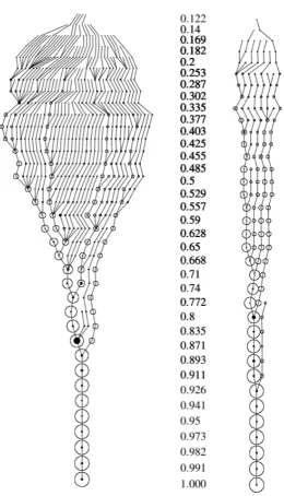
3.1 SIGMA flowchart . . . 36

3.2 Cutout image, weight map and additional background sky . . . 39

3.3 A simplified weight map . . . 41

3.4 Empirical PSF generation . . . 44

3.5 Corrected and uncorrected Source Extractor radii vs. GALFIT radii . . . 46

3.6 Final detail analysis plot for G00196053 . . . 47

3.7 Sérsic index initial starting values . . . 50

3.8 An example model output for GAMA galaxy G00092907 . . . 53

3.9 Multi-dimensional error-vector diagram . . . 56

4.1 Additional subtracted sky as a function of wavelength . . . 62

4.2 Astrometric offsets . . . 63

4.3 Recovered FWHM PSF values . . . 66

4.4 Apparent surface brightness limits . . . 67

4.5 Apparent surface brightness limits as a function of position on the sky . . . 68

4.6 Case-study model fits for G00032237 inu→K . . . 70

4.7 Case-study model fits for 9 varying magnitude galaxies in ther band . . . 72

4.8 Global results from the SIGMA common coverage sample . . . 75

4.9 A comparison between truncated Sérsic and SDSS Petrosian magnitudes . . . 77

4.10 A comparison between truncated Sérsic and GAMA photometric magnitudes . . 79

4.11 Kband Sérsic index versusu−r rest frame colour . . . 81

4.12 Sérsic index as a function of wavelength for spheroid and disk populations . . . 86

(19)

5.2 Volume-limited sample definition . . . 100

5.3 Volume-limited sample postage stamps . . . 101

5.4 Sérsick-corrections across all nine passbands. . . 104

5.5 A comparison of Sérsic and Kron-like absolute magnitudes. . . 105

5.6 Sérsic colour offsets . . . 106

5.7 Sérsic vs matched-aperture colours . . . 110

5.8 Morphological classification hierarchy . . . 112

5.9 Little Blue Spheroids: Before and After . . . 114

5.10 Eyeball classification agreement . . . 117

5.11 Example morphologies with redshift . . . 118

5.12 Correlation matrix of global measurements, by visual morphology . . . 120

5.13 Correlation matrix of global measurements, by colour . . . 124

5.14 Transition from visual morphologies into other classification schemes . . . 125

5.15 Correlation matrix of global measurements, by colour . . . 127

5.16 Galaxies which failed both GAMA photometry andK band Sérsic measurements 128 5.17 Quantitative divisions . . . 130

5.18 A matrix of scatterplots . . . 132

5.19 Principal Component Analysis . . . 134

5.20 Morphology against redshift . . . 137

5.21 Morphology against redshift by additional methods . . . 139

5.22 Single-Schechter fits to the various morphological classification methods. . . 144

5.23 Morphological agreement with Galaxy Zoo. . . 147

6.1 Bivariate-Brightness Distribution . . . 152

6.2 9 Band Morphology Luminosity Functions, Single Schechter. . . 154

6.3 9 Band Morphology Luminosity Function error ellipses. . . 157

6.4 9 Band Morphology Luminosity Functions, Double Schechter. . . 161

6.5 Ther band Morphology Luminosity Function. . . 163

6.6 Stellar Mass-to-light ratios across all nine bands . . . 165

6.7 Ther band Morphology Mass Function. . . 167

6.8 Stellar Mass Breakdown . . . 168

6.9 Number and stellar mass fractions by morphology. . . 169

6.10 Bulge-Disk Case Study - Elliptical . . . 176

6.11 Bulge-Disk Case Study - S0a . . . 177

6.12 Bulge-Disk Case Study - SB0a . . . 178

6.13 Bulge-Disk Case Study - Sbc . . . 180

6.14 Bulge-Disk Case Study - SBbcd . . . 181

6.15 Bulge-Disk Case Study - Sd . . . 182

6.16 Bulge-Disk decomposition results, Sérsic index . . . 183

6.17 Bulge-Disk decomposition results, half-light radius . . . 185

6.18 Bulge-Disk decomposition results, absolute magnitude . . . 186

6.19 Structural Luminosity Functions: Spheroid and Disk . . . 187

6.20 Structural Mass Functions: Spheroid and Disk . . . 188

6.21 Structural Luminosity Functions: Elliptical, Bulge and Disk . . . 189

6.22 Structural Mass Functions: Elliptical, Bulge and Disk . . . 190

6.23 Structural Luminosity Functions: Elliptical, Classical Bulge, Pseudo Bulge and Disk . . . 192

(20)

6.25 The Sérsic index - colour relation for bulges. . . 195

6.26 The stellar mass - size relation. . . 196

6.27 Stellar mass Breakdown . . . 198

6.28 Mass-energy density breakdown. . . 200

A.1 Morphologies: Little Blue Spheroids . . . 210

A.2 Morphologies: Ellipticals . . . 211

A.3 Morphologies: Lenticular/Early-type Spiral . . . 212

A.4 Morphologies: Barred Lenticular/Early-type Spirals . . . 213

A.5 Morphologies: Late-type Spirals . . . 214

A.6 Morphologies: Barred Late-type Spirals . . . 215

(21)

(22)

List of Tables

2.1 Bandpass central wavelengths, solar absolute magnitudes and limiting appar-ent magnitudes . . . 26 2.2 GAMA region definitions . . . 29

3.1 SIGMA modules . . . 35 3.2 Simulated parameter space grid points . . . 54

4.1 Number of detected and successfully modelled galaxies . . . 59 4.2 Sample definitions . . . 60

5.1 Sérsick-corrections across all nine bands. . . 103 5.2 Absolute Sérsic magnitude limits . . . 107 5.3 Eyeball classification results . . . 115

(23)

(24)

1

Introduction: Extragalactic Astronomy

1.1 From Cloudy Spots to Island Universes

From antiquity to the turn of the 20thcentury it was widely believed that humanity’s place in the Universe was somehow special; central to existence. As elucidated by Lynn (1901), the ancient Greek philosopher Democritus (450–370 BC) first proposed that the white band across the night sky which we now refer to as the Milky Way was composed of many stars much like our own. This theory was confirmed in 1610 by Galileo Galilei (1564–1642) who was able to magnify the Milky Way through a telescope and resolve the fainter stars from which it is comprised. The realisation that our own star is part of a much larger network of stars, or a galaxy, was fundamental in reshaping the way in which leading scientists, philosophers and theologians alike came to regard the natural world around us.

(25)

[image:25.595.72.498.79.376.2]

Figure 1.1: Lord Rosse’s depiction of M51, the Whirlpool Galaxy, as seen through his 7200_telescope

circa 1850.

time German philosopher Immanuel Kant (1724–1804) and others popularised the notion that these diffuse nebulae may in fact each be an ‘Island Universe’, a galaxy much like our own and yet spatially distant (Kant, 1755). French astronomer Charles Messier (1730–1817) began mapping these nebulae (Messier, 1774) in order to provide an atlas of sources to be avoided in his search for comets. In so doing, he produced one of the first known catalogues of extra-galactic phenomena (albeit, their distant origin unknown to him at the time). Sir Fred-erick William Herschel (1738–1822) subsequently expanded on Messier’s catalogue, creating an atlas of over 5000 galactic nebulae (Herschel, 1785).

In the mid-19thCentury, Yorkshire-born Lord William Henry Parsons, the 3rdEarl of Rosse (1800–1867), oversaw the construction of the ‘Leviathan of Parsonstown’: a 7200 telescope situated in central Ireland. The unprecedented scale of this telescope was such that upon re-observing the nebulae previously described by Messier and Herschel he was able to divide them into two distinct types, namely: elliptical nebulae and spiral nebulae. An example of one such spiral nebula is shown in a sketch made by Lord Rosse circa 1850 of M51, now known as the Whirlpool Galaxy (M51), and reproduced in Figure 1.1. Further divisions of these nebulae into elliptical and spiral types followed, e.g., Curtis (1917); Reynolds (1920); Hubble (1926).

(26)

1.1. From Cloudy Spots to Island Universes

The exceptionally named American astronomer Vesto Melvin Slipher (1875–1969) found the radial Doppler shift velocity for the Andromeda Nebula had a remarkable velocity of−300 km s−1 (Slipher, 1913). This velocity measurement put Andromeda into a league of its own when compared with other known Doppler measurements of astronomical phenomena at the time. Slipher hinted at the uniqueness of Andromeda, stating: “The magnitude of this velocity, which is the greatest hitherto observed, raises the question whether the velocity-like displacement might not be due to some other cause, but I believe we have at the present no other interpretation for it.”. A broader study made by Slipher shortly thereafter (Slipher, 1915) found that the average velocity for a sample of 15 additional spiral nebulae to be about 25 times the average stellar velocity.

The realisation of the implication of these results, and others (e.g., de Sitter, 1917; Slipher, 1917), led in 1920 to the Great Debate: a pivotal moment in the history of astronomy. The previously favoured notion that the Milky Way and the Universe are one and the same, as championed by Harlow Shapley (1885–1972), was openly challenged by Heber Doust Curtis (1872–1942) during a meeting in Washington, D.C. at the Smithsonian Museum of Natural History. Curtis was a strong advocate that Andromeda and other such nebulae were in fact extra-galactic in origin, the so called Island Universes popularised by Kant 165 years prior. He pointed to the rate of novae in those nebulous systems as anomalously high compared with observations from other parts of the Milky Way, a large flaw in Shapley’s argument if they were indeed a part of our own Galaxy. In any event, the Great Debate did not settle the matter as both parties required additional data in order to back up their claims.

(27)

[image:27.595.74.496.90.352.2]

Figure 1.2: Hubble’s measurement of the distance and radial velocity component for several nearby galaxies. This linear relation became known as Hubble’s Law, and is fundamental in our understanding of the expanding Universe. This image is taken from Figure 1 of Hubble, 1929.

reviews of Kragh & Smith, 2003; Graham, 2011).

1.2 Galaxy Morphologies

Many different schema for the classification of galaxies into morphological types have ap-peared in the literature over the last century or so. In this section I review several of the more prominent classification methodologies.

1.2.1 The Hubble Sequence

(28)

1.2. Galaxy Morphologies

continuity between classifications.

Perhaps drawing inspiration from Reynolds (1920)1, and also Jeans (1919), Hubble (1926) introduced what has since become one of the most popular means by which galaxies are clas-sified into distinct groupings; the Hubble sequence. Figure 1.3 shows a graphical represen-tation of the Hubble sequence, named the Hubble tuning fork for its distinctive two tined appearance. Galaxies are arranged into elliptical (left) and spiral (right) groupings. Elliptical galaxies are smooth, red, one-component systems that range from spheroidal (E0) to highly ellipsoidal (E7) in projection. Spiral galaxies are more complex systems containing distinctive, typically blue, spiral arm features within a flat rotating disk and emanating from a central, typically red, spheroidal bulge.

Spiral galaxies are arranged in order of the tightness of the winding in the spiral arm features and the dominance of the central bulge, from tightly wound arms with a large central bulge (Sa) to loosely wound arms with a smaller central bulge (Sc). A further distinction is made based on whether a spiral contains a bar-like feature passing through the central bulge onto which the spiral arms connect. A barred Sa-type galaxy would thus be labelled SBa.

A later introduction of an intermediate class of galaxy, S0 (Hubble, 1936c), contains char-acteristics of both populations, appearing as smooth systems with no spiral features and yet with an underlying disk like structure. These systems are called lenticulars, owing to their similarity with an optical lens. Elliptical and spiral galaxies are referred to as early-type and late-type, respectively. This naming convention does not imply an evolutionary mechanism, and indeed was never intended to (Baldry, 2008). It draws inspiration from the realm of spectroscopy, whereby simplistic spectra are referred to as ‘early’, and more complex spectra as ‘late’.

1.2.2 Revisions to the Hubble Sequence

Many authors have subsequently attempted to introduce revisions to the Hubble tuning fork, highlighting its susceptibility to misclassification owing to the effects of inclination or its over simplicity (Reynolds, 1927). It was Hubble himself who made one of the first attempts to update his classification scheme. As noted in Sandage (2005), Allan Sandage (1926–2010) came across a partially complete manuscript penned by Hubble whilst clearing out Hubble’s office following his death in 1953. The revision sought to fix the discontinuity between the S0 and SBa classes through the introduction of a SB0 class, a barred lenticular. This schema

(29)

Figure 1.3:The Hubble tuning fork, a graphical representation of the Hubble sequence.

was subsequently published in Sandage (1961) and again in Sandage et al. (1975).

A commonly used extension to the Hubble classification scheme is that advocated by French astronomer Gerard de Vaucouleurs (1918–1995). De Vaucouleurs added an additional axis to Hubble’s tuning fork such that the ring component present in some spiral systems may also be classified (de Vaucouleurs, 1959). This system is summarised in Figure 1.4. Note the distinction between barred galaxies (B), as before, and unbarred galaxies (A), now made explicit in the naming convention. This allows for intermediate structures to be termed AB if the presence of a bar is uncertain or in transition. Similarly, spiral (s) and ring (r) struc-tures may also be co-added to create therstype. Additionally, the transition lenticular galaxy type S0 is divided into E+, S0−, S00 and S0+, as per Holmberg (1958), allowing for greater resolution between these classes. The Sd type galaxy, a structure with a heavily dominant disk and little to no indication of a bulge, appears as an extension of the Sd class (Shapley & Paraskevopoulos, 1940). Beyond this, the irregular (Sm) and highly irregular (Im) classes are added.

(30)

(31)

Figure 1.5:The Kormendy revision of the Hubble tuning fork classification scheme. Elliptical galaxies are now ordered in line with how boxy or disky their isophote is. In addition, greater resolution of the bulge-to-total ratio in lenticular galaxies is added (van den Bergh, 1976). This image has been reproduced from Figure 1 of Kormendy & Bender (2012).

in lenticular bulge-to-total ratios as detailed in van den Bergh (1976). Lenticular galaxies span from bulge dominated (S0a) to disk dominated (S0c) systems, with the logical extension to pure single-component spheroidal (Sph) galaxies appended thereafter.

(32)

(33)

1.2.3 Morphology and Magnitude

One of the most fundamental measurements of a galaxy is its total luminosity, or absolute magnitude. Analysis of the luminosity function (LF), the number density of galaxies per unit luminosity interval, allows for the properties of galaxy samples to be more comprehensively studied. Early exploration of the LF led Hubble to (incorrectly) conclude that the global LF is Gaussian in shape (Hubble, 1936c,a,b). This fact was later disputed by Fritz Zwicky (1898– 1974) who was able to show that correctly accounting for the effects of selection bias changes the faint-end slope significantly (Zwicky, 1942, 1957, 1964), causing the number density to rise exponentially into the faint dwarf regime.

A distinction is often made between the LF of galaxies in the field and galaxies in over-dense regions, such as a cluster environment (Hubble & Humason, 1931; Morgan, 1961; Abell, 1965; Oemler, 1974). This division is made owing to the different morphological types found within over-dense regions when compared with morphological fractions in field galaxies (see the Morphology-Density Relation; Dressler, 1980). A full description of the LF, and its parametrisation via the Schechter luminosity function (Schechter, 1976), is given in Section 5.3.2. Figure 1.7 shows the LF for galaxies in the local field (top) and in the Virgo cluster (bottom), as indicated. This figure is reproduced from Figure 1 of Binggeli et al. (1988). Local field galaxy data has been taken from Kraan-Korteweg & Tammann (1979), whereas Virgo cluster data is from Sandage et al. (1985).

Underneath the total curves, the constituent morphological types are also indicated. These types are: elliptical, E; lenticular, S0; early-type spiral, Sa+Sb; late-type spiral, Sc; disk-dominated/Magellanic spirals, Sd+Sm; dwarf ellipticals, dE; Irregular, Irr; and blue compact dwarfs, BCD. In both the field and cluster environments, the brightest morphological types are giant elliptical galaxies, which dominate at the bright end, and hence, the high mass end. Intermediate brightness galaxies arise in the form of spirals, whereas the secondary upturn in the total LF is caused by Irregular and dwarf systems. In cluster environments, blue compact dwarfs also contribute to this bump at the faint end.

(34)

(35)

Figure 1.8: The surface brightness against absolute magnitude relations for various morphological (and structural) types. This figure is reproduced from Figure 1 of Binggeli (1994).

and lower luminosity systems, such as the compact Elliptical M32 (as indicated).

1.2.4 Galaxy Evolution Models

Observations provide key astronomical measurements of observable quantities such as that of the luminosity function (as discussed above) and the stellar mass function (see e.g., Baldry et al., 2012 and Chapter 6) and also several empirical relations such as the Morphology-Density Relation (Dressler, 1980), the Tully-Fisher Relation (Tully & Fisher, 1977) and the Faber-Jackson Relation (Faber & Jackson, 1976) (itself a projection of the Fundamental Plane for elliptical galaxies). However, it is important to put these observational measures in context by contrasting their results with those of advanced galaxy formation and evolution models. In this section, I discuss the two main means by which galaxy formation and evolution simu-lations are studied, namely: N-body simusimu-lations and semi-analytic modelling.

(36)

a cosmological constant (Λ), which denotes the energy density of empty space, and cold dark matter (CDM), which is hypothesised to be a form of weakly-interacting non-baryonic matter. A fundamental tenet of this cosmological model is the ‘cosmological principle’; that the Universe is both homogeneous and isotropic, and we as observers on Earth do not occupy a privileged or special vantage point within it. The astrophysical constants that describe the ΛCDM model are now relatively well established. We opt to use concordance cosmology

values of Ω_Λ = 0.7, Ω_M = 0.3, H0 = 70km/s/Mpc (see for example the WMAP results of

Komatsu et al., 2011) throughout this thesis unless otherwise indicated. Here, Ω_Λ is the ratio between the energy density of the cosmological constant and the critical density of the Universe (that is, the density of a Universe which exhibits a flat Euclidean-like geometry),Ω_M is the equivalent energy density for matter, andH₀is the Hubble constant.

In aΛCDM Universe, galaxies, and the large scale structure that they trace, are believed to have formed from small density perturbations in the very early Universe (Jeans, 1902). These structures continue to grow and evolve via gravitational attraction, giving rise to hierarchical growth via merging and other clustered phenomena (i.e., clusters, groups and filaments, see Efstathiou et al., 1988b; Frenk et al., 1990; Cole et al., 1994). The peak formalism devel-oped by Bardeen et al. (1986) (see also Katz et al., 1993) assumes that the earliest precursor galaxies form only at the highest peaks in the initial density field of the early Universe. The Press-Schechter formalism (Press & Schechter, 1974; Bond et al., 1991; Bower, 1991; Lacey & Cole, 1993) instead assumes that all initial density perturbations form virialised objects (dark matter haloes and galactic structure) when they grow above a given density threshold. Once an initial density distribution has been established, one may evolve their model forwards in time.

(37)

Cole et al., 1994; Rodrigues & Thomas, 1996; Somerville & Kolatt, 1999; Wechsler et al., 2002; Parkinson et al., 2008). A merger tree shows the merger history of a given structure, allowing for each progenitor mass to be successively identified back to the start of the simu-lation. An example of such a merger tree is shown in Figure 1.9, reproduced from Figure 2 of Wechsler et al. (2002). Making full use of merger information, and applying gas physics, one is able to produce realistic bulge/disk systems of a known morphology (Negroponte & White, 1983; Governato et al., 2007; Agertz et al., 2011), which is a very useful output for, e.g., the Tully-Fisher relation. Of course, N-body simulations remain extremely computationally de-manding, with practical limitations placed on particle densities and masses. Relatively large dark matter particle masses are typically employed (>∼104 solar masses), which may act to mask small-scale effects and impede on the modelling of core regions.

An additional, or perhaps complimentary approach to the study of galaxy evolution, is that of semi-analytic modelling (SAM; Cook et al., 2009, 2010b,a). SAMs adopt the merger trees mentioned above, and assign properties to each structure based on a physically moti-vated model. Instead of focusing on the gas dynamics of numerical simulations, SAMs are concerned with the global properties of galaxies, allowing for a level of description unavail-able in many contemporary numerical simulations. Assuming some initial cosmology, SAMs must aim to reproduce the low-redshift galaxy properties observed today, such as the Tully-Fisher Relation, the luminosity function and the relationship between luminosity, colour and metallicity. Common SAM components are gas cooling mechanisms; star formation rate his-tory (Lilly et al., 1996; Madau et al., 1996); feedback; metal enrichment; black hole growth; stellar population synthesis, and; mergers via dark matter merging trees (see above, and, e.g., Lacey & Cole, 1993).

(38)

[image:38.595.182.443.155.610.2]

Figure 1.9:Structural merger trees for two distinct halos, reproduced from Figure 2 of Wechsler et al. (2002). The merger history of a cluster mass halo (M =2.8×1014M, left) and a galaxy mass halo

(M = 2.9×1012M, right) is shown progressing from the early Universe (top) to the present day

(39)

1.3 The Sérsic Profile

Measuring and quantifying the surface brightness profile of galaxies has been a useful tool for further exploration of intrinsic galactic properties for some time. As was established by Naim et al. (1995), visual galaxy classification remains a subjective measure of the property of a galaxy. Naim found that whilst individual observers agree on the whole, the scatter about each classification can be prohibitively large. Replacing subjective morphological classifica-tions with something more quantitative, such as analysis of the surface brightness profile, is a natural and logical extension of extragalactic analyses.

It is commonplace to approximate the disks of spiral galaxies with an exponential profile (Freeman, 1970; Kormendy, 1977b; Andredakis & Sanders, 1994), as this seems to provide a good indication of the light distribution in those systems (e.g., Bland-Hawthorn et al., 2005). Early-type galaxies are not so standardised. The simplistic model of Plummer (1911), initially developed to model the distribution of light in globular clusters, found some early use in modelling the surface brightness distribution of elliptical galaxies. Similarly, the King profile (King, 1962, 1966; Elson, 1999), again developed to model globular cluster light profiles, is now used by some observers to model the faint nucleated cores of early-type galaxies (e.g., Ferrarese et al., 2006). The Hubble-Reynolds law (Reynolds, 1913; Hubble, 1930; Binney & Tremaine, 2008) was one of the first light profile models developed specifically for elliptical galaxies (or elliptical nebulae as they were known). It is given by

I(r) = I0

(1+r/rH)2

(1.1)

where I is the luminosity, I0 is the central luminosity, r is the distance from the centre and

r_H is some scaling radius. In many regards, this profile fit has now largely been superseded by de Vaucouleurs’ law: logI(r)∝r1/4 (de Vaucouleurs, 1948). Whilst there is no theoretical justification for de Vaucouleurs’ law, it has been extremely successful in modelling the surface brightness light profiles of elliptical galaxies and classical bulge components (e.g., Kormendy, 1977a). De Vaucouleurs himself is said to have described it as “a good French curve”.

(40)

1.3. The Sérsic Profile

equation provides the intensityI at a given radiusr as given by:

I(r) =Ieexp

−bn

_r

r_e

1/n

−1

(1.2)

whereIeis the intensity at the effective radiusre, the radius containing half of the total light,

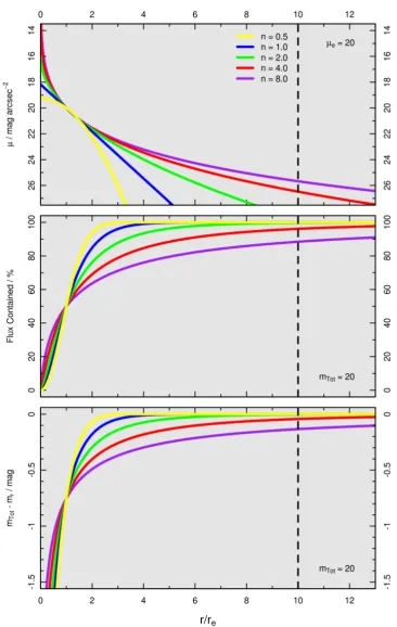
andnis the Sérsic index which determines the shape of the light profile (see Figure 1.10). The value of bn is a function of Sérsic index and is such thatΓ(2n) =2γ(2n,bn),2 whereΓandγ

represent the complete and incomplete gamma functions respectively (Ciotti, 1991). Varying the Sérsic index parameternallows one to model a wide range of galaxy profile shapes, with n = 0.5 giving a Gaussian profile, n = 1 an exponential profile suitable for galactic disks, andn=4 a de Vaucouleurs profile commonly associated with massive spheroidal components such as elliptical galaxies.

1.3.1 What Happens Below the Limiting Isophote?

Whilst the surface brightness profile of some galaxies behaves as expected out to very faint magnitudes (e.g., NGC 300: Bland-Hawthorn et al., 2005; Vlaji´c et al., 2009, NGC 7793: Vlaji´c et al., 2011), the potential myriad of phenomena present in the outer wings of many systems may cause deviations away from a typical light profile. These include truncated and anti-truncated disks (Erwin et al., 2005; Pohlen & Trujillo, 2006), UV excesses (Bush et al., 2010), tidal debris, halos (Barker et al., 2009; McConnachie et al., 2009) and minor merger fossil records (Martínez-Delgado et al., 2010). In fact, the outer regions of galaxies may defy any systematic profile fitting into a restricted number of structures. The accuracy of any estimation of the background sky and gradients therein will also no doubt affect analyses of these outer structures.

1.3.2 Fixed vs Model Aperture Photometry

Since it is not known exactly how the light profile of a galaxy behaves at large radii away from the core regions, several traditional methods of aperture-based flux estimation have been de-vised. Magnitudes within these isophotal radii, not surprisingly, systematically underestimate the total galaxy light, in particular, relative to the Sérsic magnitude (e.g., Caon et al., 1990, 1993). Graham & Driver (2005) show for example that Kron magnitudes may underestimate the total galaxy flux by as much as_∼ 55% dependent upon choice of the multiple of Kron radii chosen to integrate out to and the profile shape of the galaxy. The comparative value 2_b

ncan trivially be calculated within R using the relationbn=qgamma(0.5, 2n), where qgamma is the quantile

(41)

[image:41.595.101.468.94.673.2]

(42)

for Petrosian magnitudes is considerably worse, underestimating flux by as much as_∼95% in the extreme case of a high-Sérsic index object integrating out to thrice the Petrosian radius. In addition to these considerations, belowµ_B=27 mag arcsec−2environmental effects begin to play an increasing role in profile shape determination.

In contrast to traditional aperture methods, studies have repeatedly shown the strength of Sérsic profiling for the majority of elliptical galaxies (e.g., Caon et al. (1993); Graham & Guzmán (2003); Trujillo et al. (2004); Ferrarese et al. (2006)). Tal & van Dokkum (2011) support this viewpoint, showing the light profiles of massive ellipticals are well described by a single Sérsic component out to _∼8 r_e, with evidence for additional flux beyond these radii possibly related to unresolved intra-group light. With regards to disk systems, Bland-Hawthorn et al. (2005) use one of the deepest imaging studies of spiral galaxy NGC 300 to show that an exponential profile (n=1) is a good descriptor of its light profile out to_∼17 r_e. From a sample of 90 face-on late-type galaxies, Pohlen & Trujillo (2006) confirm the accuracy of Sérsic profiling down toµ=27 mag arcsec−2, and suggest up to 10% of their sample show evidence for a deviation from a standardn=1 Sérsic fit (Type I), instead showing a broken exponential profile. These breaks appear in the form of either adownbending(Type II; steeper flux drop-off) orupbending (Type III; shallower flux drop-off) with increasing radii. Impor-tantly, this study also suggests this observed feature is independent of local environment.

1.3.3 Accounting for Uncertainty

(43)

display any redshift dependence however, and is trivial to subsequently recorrect if desired. Corrections are typically minor for most galaxies, becoming most acute in high-index systems (see Figure 1.10).

A sufficiently large truncation radius must be adopted to provide a close estimate of total flux without extrapolating too deep into the region of uncertainty. Sloan Digital Sky Survey (SDSS; Abazajian et al. 2009) model magnitudes (magnitudes based on the best fitting expo-nential/de Vaucouleurs profile) employ a smooth truncation at 3r_edown to zero flux at 4 r_e for exponential (n=1) profiles and 7r_e down to zero flux at 8r_efor de Vaucouleurs (n=4) profiles.

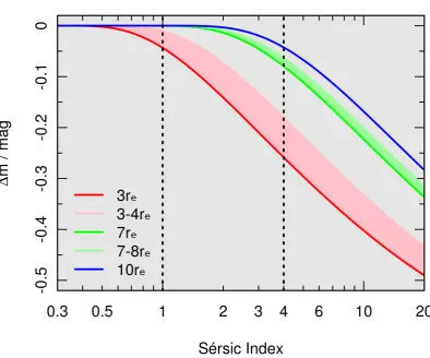
We advocate a sharp truncation radius of 10r_efor all Sérsic indices (shown by a vertical dashed line in Figure 1.10), which corresponds to an isophotal detection limit of µ_r _∼ 30 mag arcsec−2, the limit to which galaxy profiles have been studied. Figure 1.11 shows the magnitude offset between the Sérsic profile integrated to infinity and that truncated at 3, 7 and 10 re as red, green and blue lines respectively, with shaded areas representing the SDSS

tapered limits. A 10 r_e truncation gives a negligible magnitude offset for n = 1, and an offset of∆m∼ −0.04 forn=4, with larger corrections for higher Sérsic indices. Figure 1.10, middle panel, shows the flux contained within 10r_e(dashed vertical line) for various values of n. Given a 10retruncation,∼100% of the pre-truncation flux is retained forn=1, reducing

to 96.1% forn=4. Sérsic magnitudes truncated at 10r_eare adopted as the standard Sérsic magnitude system throughout this thesis.

1.3.4 Magnitude Comparisons

Figure 1.12 shows the offsets between various magnitude systems discussed previously (SDSS Petrosian and Model magnitudes) and Sérsic magnitudes (integrated to infinity and 10 re)

as a function of Sérsic index (Kelvin et al., 2012). When comparing Sérsic magnitudes in-tegrated to infinity against SDSS Petrosian magnitudes we see the two systems are in good agreement until n_r _∼2, beyond which the magnitude offset relation begins to turn-off from the∆m=0 relation. This trend argues that Sérsic magnitudes are recovering an additional ∼ 0.4 magnitudes for an n_r = 8 object which would otherwise have been missed by tradi-tional photometric methods. For the reasons previously discussed however, this value should be taken as a rough (~upper) estimate of the true amount of flux missed for an object of a given Sérsic index. Truncating the Sérsic index at 10 re reduces the scale of this turn-off,

(44)

[image:44.595.116.511.225.553.2]

(45)

providing some measure of turn-off beyond this point. We would expect SDSS Petrosian mag-nitudes, or indeed any aperture-based photometry, to underestimate total flux for objects with large wings, and so this result is not surprising and a good indication that truncated Sérsic magnitudes are performing as expected.

The final panel in Figure 1.12 compares truncated Sérsic magnitudes against SDSS model magnitudes. The SDSS force fit either an exponential or de Vaucouleurs profile fit (marked on the figure by dashed grey lines) depending upon which profile an individual galaxy most approximates during their calculations. We see clearly the inadequacy of model magnitudes when a more comprehensive Sérsic magnitude is available, with the population of galaxies split into two distinct sub-populations based upon their SDSS forced fit. For a galaxy atn=2 for example, the model magnitude for the galaxy may be offset from its correct magnitude by as much as∆m=±0.3 magnitudes, with larger offsets observed for high index galaxies. If one constructs a line of best fit for each of these two artificial sub-populations then one finds that the lines pass through ∆m = 0 and n = 1 or 4 as appropriate, confirming that SDSS model and truncated Sérsic magnitudes agree for exponential and de Vaucouleurs type galaxies.

1.4 Concluding Remarks

(46)

[image:46.595.160.476.90.616.2]

1.4. Concluding Remarks

Figure 1.12:A series of plots displaying offsets between various magnitude systems as a function ofr -band Sérsic index, with the data points coloured according to theiru₋rrest colour, as shown. Contours range from the 10th_{percentile to the 90}th_{percentile in 10% steps. (top) The Sérsic profile integrated}

out to infinity minus the SDSS Petrosian magnitude and; (middle) the Sérsic profile truncated at 10re

minus the SDSS Petrosian magnitude. These figures show how Sérsic profiling is able to recover flux in the wings of galaxies that would otherwise be missed by traditional aperture based methods, such as Petrosian apertures. (bottom) The Sérsic profile truncated at 10reminus the SDSS model magnitude.

(47)

(48)

2

Survey Data

Imaging and Spectroscopic data from multiple surveys has been collected, collated and processed in order to provide a consistent multi-wavelength dataset with which to perform analysis upon. I now discuss the origins of these data.

2.1 The Sloan Digital Sky Survey (SDSS)

(49)

u g r i Z/z Y J H Ks/K λ(nm) 355 470 620 750 880/895 1030 1250 1630 2150/2200

M(AB) 6.38 5.15 4.71 4.56 4.54 4.52 4.57 4.71 5.19

SDSS 22.0 22.2 22.2 21.3 20.5

KIDS 24.8 25.4 25.2 24.2

UKIDSS-LAS 21.1 20.9 20.2 20.3

VIKING 23.1 22.3 22.1 21.5 21.2

Table 2.1: Central wavelengths, solar absolute magnitudes and limiting apparent magnitudes for a selection of current- and next-generation wide-area surveys. Solar absolute magnitudes are taken from Table 1 of Hill et al. (2010), and represent the SDSS/UKIDSS bandpasses. Note that all limiting depths are at 5σ(with the exception of SDSS, which are 2σ) and are on the AB magnitude system.

(50)

2.2. The UKIRT Infrared Deep Sky Survey (UKIDSS)

The SDSS camera contains 6 columns of CCD chips with 5 chips per column, one for each passband. Each chip is 2048×2048 pixels in size at a resolution of 0.396 arcseconds pixel−1, giving an angular size of 13.51_×13.51 arcminutes per CCD chip. The angular space between columns is slightly smaller than the field of view of a single chip (86%), which is designed as such in order that two successive observations may be interleaved to form a contiguous region. Observations are taken using a drift-scanning technique whereby the pointing of the telescope remains fixed to a celestial great circle, with the CCD columns arranged such that the image of an object moves along a single column, being detected in every filter separately. Each CCD is constantly read out at the same rate as the procession of the night sky, with a total effective exposure time of 53.9 seconds per CCD. A single drift-scan produces an SDSS strip, and two interleaved strips produce astripe. Stripes are subsequently cut into square fields before being served to the wider astronomy community via the SDSS website1.

Wide area surveys such as the SDSS are well served by the combination of the drift-scanning technique and continuous CCD readouts as it allows large swathes of the night sky to be observed on a given night without losing time closing the shutter between pointings. However, variation in seeing between the two strips that constitute a stripe has the potential introduce large-scale anomalies in the quality of the imaging data, as can be seen in Figure 2.2. Typically, the FWHM of SDSS data lies in the range 0.9 to 1.6 arcseconds (see Figure 4.3).

2.2 The UKIRT Infrared Deep Sky Survey (UKIDSS)

The UKIRT Infrared Deep Sky Survey (UKIDSS; Dye et al., 2006; Lawrence et al., 2007) is a near-infrared (NIR) survey using the UKIRT Wide Field Camera (WFCAM; Casali et al., 2007) instrument on the 3.8 m United Kingdom Infrared Telescope (UKIRT) situated on Mauna Kea, Hawaii. The UKIDSS Large Area Survey (UKIDSS-LAS) is one of five sub-surveys in UKIDSS, providing imaging data across approximately 4000 deg2 in theY, J, H andK bands, whose central wavelengths are approximately 880, 1030, 1250, 1630 and 2200 nm respectively and with limiting AB magnitudes at 5σ of 21.1, 20.9, 20.2 and 20.3, respectively. These values are summarised and compared in Table 2.1. Note that UKIDSS-LAS magnitudes have been converted from their native Vega calibration onto a standard AB magnitude system in order that they may more easily be compared with other surveys. Conversions are made using the relation mAB = mVega+moffset, where moffset values are 0.634, 0.938, 1.379 and 1.900 for

(51)

Y J H Krespectively (see Hewett et al., 2006). The relative throughput for each band is shown in Figure 2.1.

WFCAM consists of four 2048×2048 pixel CCDs at an apparent angular resolution of 0.4 arcseconds pixel−1 (equating to 13.65_×13.65 arcminutes per CCD) arranged in a square formation with a gap of 12.83 arcminutes between CCDs. This formation allows for four unique pointings (pawprints) to be co-added to form a contiguous 0.9_×0.9 degree tile.

Variable UKIDSS coverage across the three GAMA regions (see below) leaves a noticeable imprint in the coverage map shown in Figure 2.2. Several of these frames were manually removed after being checked for imaging accuracy and found to contain corrupt imaging data, such as a frame which has tracked badly or is out of focus.

2.3 The VISTA Kilo-Degree Infrared Galaxy Survey (VIKING)

The VISTA Kilo-Degree Infrared Galaxy Survey (VIKING; Sutherland et al., in prep.) survey is a NIR effort to map 1500 deg2 of the sky using the VISTA Infrared Camera (VIRCAM; Dalton, 2006) atop the 4 m Visible and Infrared Telescope for Astronomy (VISTA; Emerson et al., 2006; Arnaboldi et al., 2007; Emerson & Sutherland, 2010) situated at ESO’s Cerro Paranal Observatory, Chile. VIKING takes observations in 5 bands, namely, Z Y J H and Ks (note thatK-short is the same filter used with 2MASS, but not that used for UKIDSS). These bands have central wavelengths of 880, 1020, 1250, 1650 and 2150 nm respectively, with limiting AB depths of 23.1, 22.3, 22.1, 21.5 and 21.1 magnitudes, respectively. These values are summarised and compared in Table 2.1. The relative throughput, assuming standard atmospheric conditions at the site, is shown in Figure 2.1.

The VIRCAM instrument consists of sixteen 2048_×2048 CCDs at a resolution of 0.339 arcseconds pixel−1 arranged into a 4×4 square formation (a pawprint). The separation between columns is 90% the width of a single CCD, whereas the separation between rows is 42.5%. This formation allows for 6 pawprints to be interleaved in order to form a contiguous 1.5 deg2 region on the sky.

(52)

2.4. Galaxy and Mass Assembly (GAMA)

Region RA (J2000) Dec. (J2000) rl im No b j zcomp

G09 129◦_.0_{< α <}₁₄₁◦_.0 ₋₁◦_.0_{< δ <}₃◦_.0 _{19.4 (19.8)} _{30, 289 (48, 548)} _{99.23% (79.36%)}

G12 174◦_.0_{< α <}₁₈₆◦_.0 ₋₂◦_.0_{< δ <}₂◦_.0 _{19.8 (19.4)} _{50, 868 (32, 747)} _{99.12% (99.39%)}

G15 211◦_.5_{< α <}₂₂₃◦_.5 ₋₂◦_.0_{< δ <}₂◦_.0 _{19.4 (19.8)} _{33, 205 (51, 217)} _{98.95% (79.27%)}

Table 2.2:GAMA region definitions. The GAMA main survey definitions are based on SDSS extinction corrected r-band Petrosian magnitude limits, the depth of which varies between r = 19.4 mag in G09/G15 andr=19.8 mag in G12. Comparison magnitude limits are shown in brackets for reference. Number counts and redshift completeness are based on objects which passed star-galaxy separation in the GAMA TilingCatv11 (see Baldry et al. (2010) for further details).

2.4 Galaxy and Mass Assembly (GAMA)

The GAMA survey is a combined spectroscopic and multi-wavelength imaging programme de-signed to study spatial structure in the nearby (z<0.25) Universe on scales of 1kpc to 1Mpc (see Driver et al. 2009 for an overview). The survey, after completion of Phase I, consists of three regions of sky each of 4 deg (Dec)_×12 deg (RA), close to the equatorial region, at approximately 9h(G09), 12h(G12) and 14.5h (G15) Right Ascension (see Table 2.2 and Fig-ure 2.2 for reference). The three regions were selected to enable accurate characterisation of the large scale structure over a range of redshifts and with regard to practical observing con-siderations and constraints. They lay within areas of sky scheduled for survey by both SDSS (Abazajian et al. 2009) as part of its Main Survey, and UKIRT as part of the UKIDSS Large Area Survey (UKIDSS-LAS; Lawrence et al., 2007). These data provide moderate depth and resolu-tion imaging data inug r izY J H Ksuitable for analysis of nearby galaxies. The accompanying spectroscopic input catalogue was derived from the SDSS PHOTO parameter (Stoughton et al., 2002) as described in Baldry et al. (2010). The GAMA spectroscopic programme (Robotham et al., 2010) commenced in 2008 using AAOmega on the Anglo-Australian Telescope to ob-tain distance information (redshifts) for all galaxies brighter than r<19.8 mag. The survey is_∼ 99 percent complete to r < 19.4 mag in G09 and G15 and r < 19.8 mag in G12 (see Table 2.2, column 6), with a median redshift of z ∼ 0.2. Full details of the GAMA Phase I spectroscopic programme, key survey diagnostics, and the GAMA public and team databases are given in Driver et al. (2011).

2.4.1 Data Processing and Mosaicing

(53)

(54)

2.4. Galaxy and Mass Assembly (GAMA)

2002). Associated weight map mosaics (swpwt) are also constructed. Note that at the time of writing only theK band G09 VISTA data is available, and so the process described below is currently only applicable to the SDSS and UKIDSS data. In constructing these large mo-saics, all native reduced frames are downloaded from the respective archives (SDSS DR7 and ROE/WFAU) and scaled to a single uniform zero point (30 mag arcsec−2). For SDSS, the input data are the corrected (fpC) Data Release 7 (DR7) files, with the data having already been bias subtracted and flat-fielded as part of the SDSSframespipeline (Stoughton et al., 2002, Section 4.4). The UKIDSS-LAS data has been collected from the UKIDSS Early Data Release (EDR; Dye et al., 2006) and data releases 1 and 2 (DR1; Warren et al., 2007b, DR2; Warren et al., 2007a). The UKIDSS project is defined in Lawrence et al. (2007). UKIDSS uses the United Kingdom Infrared Telescope Wide Field Camera (WFCAM; Casali et al., 2007). The photometric system is described in Hewett et al. (2006), and the calibration is described in Hodgkin et al. (2009). The pipeline processing and science archive are described in Irwin et al (in prep.) and Hambly et al. (2008).

Once these input data have been obtained and calibrated, SWARPis then used to combine

them into a single image mosaic at a resolution of 0.33900arcseconds per pixel in the TAN pro-jection system (Calabretta & Greisen, 2002) centred within each GAMA region as appropriate. Note that we are using version 2 SWARPmosaics scaled to a slightly higher resolution (0.33900)

than the previous version 1 mosaics (0.400) as described in Hill et al. (2011). This increased resolution has been chosen to match that which is expected for future VISTA VIKING data releases, allowing easy cross-wavelength cross-facility comparison of data. Original SDSS and UKIDSS resolutions of 0.39600and 0.400respectively place a limit on how high one is able to artificially increase the resolution of mosaiced data, requiring increasing amounts of interpo-lation with increasing artificial resolution. Further details may be found in Liske et al. (in prep.). Version 2 mosaics are a minimum of 193900×79700 pixels each, with each individual FITS file_∼60GB in size. The process used to create the version 2 mosaics is identical except the regions have been expanded in preparation for GAMA Phase II operations and at higher resolution in preparation for matching to VISTA data in due course2.

As part of the SWARP mosaicing process the background is removed on each individual

frame prior to merging using a 256_×256 pixel median filtered mesh which itself is median filtered within a 3_×3 mesh. The original SDSS and UKIDSS data are typically held in chunks

2_{These larger, higher-resolution version 2 mosaics will be released shortly via the GAMA website:}

(55)

of 2048_×1489 pixels and 2072_×2072 pixels respectively, at comparable pixel scales (SDSS: 0.39600/pixel, UKIDSS: 0.400/pixel). At the native pixel resolution the mesh size therefore equates to 101.400_×101.400and 102.400_×102.400respectively and so structures with half-light radii less than∼1700should be unaffected by the background smoothing. Note that UKIDSSJ band data and selected UKIDSS EDR fields in bothH andKbands were microstepped. These data are typically stored in chunks of 4103×4103 pixels at a native resolution of 0.200/pi x el, giving a mesh size of 51.200_×51.200.

In addition to the science image frames are the associated weight maps. Because of the zero-point normalisation across all data, and overlapping edge duplication in the SDSS data, the actual weight map values produced by SWARPare an approximation of their correct value.

(56)

3

SIGMA: Structural Investigation of Galaxies via

Model Analysis

(57)

3.1 SIGMA Setup

The only inputs required by SIGMA are the imaging data itself and the locations of the primary galaxies within them which are to be modelled. All additional parameters and starting values for extra neighbouring objects in the field of view (secondary objects), including PSF evalua-tion, are determined by SIGMA on the fly on a per-galaxy basis. All scripting and additional programming is written in the open source and freely available R programming language (R Development Core Team, 2010).

Typically, SIGMA is run across multiple-processors, and will output a Comma-Separated Variable (CSV) catalogue, which may subsequently be opened and converted in TOPCAT (Tay-lor, 2005). The average run-time to profile a galaxy with a single-component (single-Sérsic) fit is 15 seconds per processor1 sustained over several hundred thousand objects.

3.1.1 Startup

On starting SIGMA, a number of input options can be specified. Some of these are essential in its use, whereas others are designed for testing purposes only. The available input options can be found in the help document, reproduced (from SIGMA version 0.9-0) below.

Listing 3.1:SIGMA help lists the available input options that may be specified when starting SIGMA.

$ sigma -h

--- SIGMA Version 0.9 -0 -- 23 Jul 2010

DESCRIPTION

SIGMA ( Structural Investigation of Galaxies via Model Analysis ) is a 2 dimensional fitting code taking inputs from the GAMA SWarped regions and producing models using the GALFIT software .

OPTIONS

-a A - append A to output log files -b A - A- band ( default : r)

-c A - input catalogue [ img / csv ] ( needs at least RA & DEC ) -d - show program defaults

-e # - error generation method (1= GALFIT , 2= BOOTSTRAP ) -h - help ( this screen )

-i - interactive mode

-m - make a plot of output . fits files ( png format ) -n A - output catalogue name

-o - no headers in output catalogue , only data -p # - number of sub - processes to spawn

-r # - number of bootstrap runs to generate errors in GALFIT -s # # - subsample , from lower to upper quantile

-t #,# - principle allowed multi - component types (eg: 1 ,2 ,5 ,10) -v - version number

1_{Using current computer hardware at the University of St Andrews. This consists of a 16 core Intel Xeon E5520}

(58)

3.2. Modules

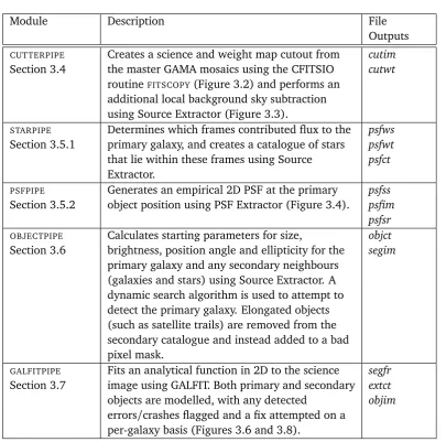
Module Description File

Outputs

CUTTERPIPE

Section 3.4

Creates a science and weight map cutout from the master GAMA mosaics using the CFITSIO routineFITSCOPY(Figure 3.2) and performs an

additional local background sky subtraction using Source Extractor (Figure 3.3).

cutim cutwt

STARPIPE

Section 3.5.1

Determines which frames contributed flux to the primary galaxy, and creates a catalogue of stars that lie within these frames using Source Extractor. psfws psfwt psfct PSFPIPE Section 3.5.2

Generates an empirical 2D PSF at the primary object position using PSF Extractor (Figure 3.4).

psfss psfim psfsr

OBJECTPIPE

Section 3.6

Calculates starting parameters for size,

brightness, position angle and ellipticity for the primary galaxy and any secondary neighbours (galaxies and stars) using Source Extractor. A dynamic search algorithm is used to attempt to detect the primary galaxy. Elongated objects (such as satellite trails) are removed from the secondary catalogue and instead added to a bad pixel mask.

objct segim

GALFITPIPE

Section 3.7

Fits an analytical function in 2D to the science image using GALFIT. Both primary and secondary objects are modelled, with any detected

errors/crashes flagged and a fix attempted on a per-galaxy basis (Figures 3.6 and 3.8).

[image:58.595.112.518.83.484.2]

segfr extct objim

Table 3.1: Summary of the modules that comprise SIGMA, a brief description of their purpose, and a list of the file outputs produced by each.

-x # - GAMA ID -y # - SIGMA ID -z # - SDSS OBJID

CONTACT Lee Kelvin

University of St Andrews lsk9@st - andrews .ac.uk

3.2 Modules

(59)

Load SIGMA & input catalogue

Filter the input catalogue

based on search criteria

(e.g.: r < 19.4)

Prepare input catalogue Spawn additional instances of SIGMA and split the input

catalogue equally between them Load SIGMA modules Multiple processors? Y N Object filter? Y For each galaxy: create primary galaxy file structure N Define 1201×1201 pixel region around primary Correct measured radii for the effects of seeing and

ellipticity Return null results for remaining data columns Cutout creation CUTTERPIPE Star detection STARPIPE PSF creation PSFPIPE First pass: < 10 stars detected? Define 1501×1501 pixel region around primary Object detection OBJECTPIPE Y N Primary object detected? N Y Last galaxy? N Galaxy fitting GALFITPIPE Store output data in SIGMA main catalogue

Compress file outputs into a tarball and tidy

folder Create R scripts allowing

future user to construct analysis plots Multiple processors? Y Join together multi-processor catalogues Finish SIGMA N Y Task Decision Module

S I G M A

Structural Investigation of Galaxies via Model Analysis

(60)

3.3. Master Script

3.3 Master Script

When initialising SIGMA a number of options are specified, such as band(s), naming con-ventions, number of processors and model fit types. SIGMA’s master script handles these requests, and sets up the data and directories for further subsequent processing. To begin, SIGMA’s master script loads into memory the entirety of the input catalogue (GAMA Tiling Catalogue) and defines a naming convention for each primary object based on its own unique identifier (SIGMA_INDEX). A template master CSV catalogue is created into which all of the output data will accumulate as SIGMA loops across each primary galaxy. Once the setup is complete, the master script will loop across every primary object in turn. If for any reason a primary galaxy causes a software crash, with attempted fixes as detailed in subsequent sec-tions unsuccessful, SIGMA will report how far it was able to progress and record a NULL result before proceeding on to the next primary galaxy in the input catalogue. We now discuss each module from Table 3.1 in turn.

3.4 Image Processing

TheCUTTERPIPEmodule creates and prepares the fitting image to be fed into GALFIT. Version 2

mosaics of the three GAMA regions are used as an input toCUTTERPIPE, with a full description

of the construction and manipulation of these files given in Hill et al. (2011) and summarised in Section 2.4.1.

CUTTERPIPE’s first task is to create the core cutout of the science image and its associated

weight map. Using the WCS information stored in the FITS header of the appropriate mo-saiced image,CUTTERPIPEconverts the input RA/DEC into an x/y pixel coordinate. The upper

and lower limits of a 1201_×1201 pixel (_∼40000_×40000) region centred on the primary galaxy are determined. Using the NASA HEASARC package’s CFITSIO subroutine library, namely the routineFITSCOPY, cutouts centred on the primary galaxy on both the mosaiced science image,

swpim, and mosaiced weight map, swpwt, are created. These cutouts are named cutim and cutwtrespectively. FITSCOPY was found to be the most efficient routine at dealing with the

large mosaic files in use, able to quickly analyse the input file and read into memory only the relevant area of interest, thereby reducing file handling time significantly.

(61)

in the fitting process by GALFIT in order to generate a sigma-map (an image showing the 1σconfidence interval at every pixel). CUTTERPIPE reverts these to typical pre-mosaic values

which are more appropriate for a smaller single image rather than a larger mosaic. GAIN, RDNOISE, NCOMBINE and EXPTIME are set to values of 0.5, 3, 1 and 1 respectively. These typical values are averages taken from pre-mosaiced data frames.

An estimate of the local background sky is then made with Source Extractor (v2.8.6; Bertin & Arnouts, 1996) using a variable background grid in a 3×3 mesh configuration. Possible grid sizes are 32_×32, 64_×64 and 128_×128 pixels. The size of the chosen background grid is dependent upon the size of the primary galaxy: larger galaxies will lead to a larger background grid being used so as not to contaminate the sky estimate with galaxy flux. An initial basic estimate of the total size of the primary is given by:

r_{t ot}=2×r99 (3.1)

where r₉₉is the radius of the primary galaxy which contains 99% of the flux. This is obtained from the Source Extractor parameter FLUX_RADIUS, setting PHOT_FLUXFRAC=0.992. Note that a size estimate produced by Source Extractor in this manner is known to be smaller than the true galaxy value, scaling as a function of Sérsic index and thus absolute magnitude. This effect has been accounted for, and does not adversely affect any of the analysis or results here presented. If rt ot < 128, CUTTERPIPE rounds up rt ot to the nearest available grid size

and performs a background subtraction on the science image as appropriate. If r_{t ot} _≥ 128, no background subtraction is necessary, as the master GAMA mosaics have a 256_×256 pixel background grid subtraction already applied. Although the value of actual subtracted sky varies with position on the cutout image, the specific value at the position of the primary galaxy,ρskyis recorded through the Source Extractor parameter BACKGROUND. The error on

the background sky estimate is then given by:

∆ρsk y=

σsky p

0.9×n_x×n_y (3.2)

where σ_sky is the RMS of background sky counts across the cutout, and nx and ny are the

dimensions of the cutout in thexand ydimensions respectively. The background sky typically encompasses_∼90% of any given cutout, and hence a factor of 0.9 is introduced into the above

2_{Typically, Source Extractor FLUX_RADIUS refers to}_r

The structure of galaxies : the division of stellar mass by morphological type and structural component

STELLAR MASS BY MORPHOLOGICAL TYPE AND

STRUCTURAL COMPONENT

Lee Steven Kelvin

A Thesis Submitted for the Degree of PhD

at the

University of St Andrews

2013

Full metadata for this item is available in

Research@StAndrews:FullText

at:

http://research-repository.st-andrews.ac.uk/

Please use this identifier to cite or link to this item:

http://hdl.handle.net/10023/3689

The Structure of Galaxies

The Division of Stellar Mass by Morphological Type and Structural Component

Lee Steven Kelvin

Submitted for the degree of Doctor of Philosophy in Astrophysics

Declaration

Copyright Agreement

Abstract

Acknowledgements

Contents

List of Figures

List of Tables

1

Introduction: Extragalactic Astronomy

1.1

From Cloudy Spots to Island Universes

1.2

Galaxy Morphologies

1.2.1

The Hubble Sequence

1.2.2

Revisions to the Hubble Sequence

1.2.3

Morphology and Magnitude

1.2.4

Galaxy Evolution Models

1.3

The Sérsic Profile

1.3.1

What Happens Below the Limiting Isophote?

1.3.2

Fixed vs Model Aperture Photometry

1.3.3

Accounting for Uncertainty

1.3.4

Magnitude Comparisons

1.4

Concluding Remarks

2

Survey Data

2.1

The Sloan Digital Sky Survey (SDSS)

2.2

The UKIRT Infrared Deep Sky Survey (UKIDSS)

2.3

The VISTA Kilo-Degree Infrared Galaxy Survey (VIKING)

2.4

Galaxy and Mass Assembly (GAMA)

2.4.1

Data Processing and Mosaicing

3

SIGMA: Structural Investigation of Galaxies via

Model Analysis

3.1

SIGMA Setup

3.1.1

Startup

3.2

Modules

S I G M A

3.3

Master Script

3.4

Image Processing