Effective determination of cyclic visco plasticity material properties using an optimisation procedure and experimental data exhibiting scatter

A Method for the Effective Determination of Cyclic-Visco-Plasticity Material Properties Using an Optimisation Procedure and Experimental Data Exhibiting Scatter

J. P. Rouse*, C. J. Hyde, W. Sun, T. H. Hyde

Department of Mechanical, Materials and Manufacturing Engineering, University of Nottingham, University Park, Nottingham, NG7 2RD, UK.

*_{Corresponding Author – email: [email protected]}

Tel: +44 (0) 115 84 67682

Key words: Chaboche; Optimisation; Low Cycle Fatigue; Creep.

Abstract

It may be inevitable in the design and analysis of most high temperature components (such as power industry pipe work) that variations in load and/or temperature will occur in normal operation. This presents

complications in the prediction of the response of such components due to potential hardening or softening effects caused by the accumulation of plastic strain [1, 2]. Furthermore, interactions between hardening (or softening) behaviour and creep may be observed, particularly in high temperature applications. In this paper the Chaboche model is described as it has the potential to represent this type of behaviour [1, 3]. An optimisation procedure for fine tuning material constants is developed and presented. This is a key step as the determination of initial estimates requires several assumptions to be made. Several potential pitfalls in optimisation procedures are described and addressed, mainly through the application of experimental data cleaning as a pre-processing procedure. This removes unavoidable experimental scatter that inhibits optimisation. Investigations into the effects of variations in the initial conditions on optimised material constant values and the number of data points selected on computational times are made to aid in the application of similar optimisation procedures. The superior fitting given by the implementation of an optimisation procedure is verified by applying it to the results of strain controlled cyclic tests of a P91 steel at 600°C.

1. Introduction

High temperature components, such as steam pipe work used extensively in the power industry, may inevitably experience not only fluctuations in loading (internal pressure or system loading in the case of pipe work), but also fluctuations in temperature. Focusing on the future trends of power plant operation, these fluctuations will become more pronounced as operators attempt to generate in a highly strategic manner, maximising generation effectiveness [4]. Variations in loading or temperature present serious complications when analysing such components due to the cyclic hardening and/or softening behaviour of materials if the material works within the plastic range. Models that can predict this behaviour, while allowing for the creep response to be included as well, are therefore of great interest to many industries. With greater predictive accuracy, power generation plant, for example, could be operated with confidence in a more arduous fashion, potentially allowing for greater plant flexibility.

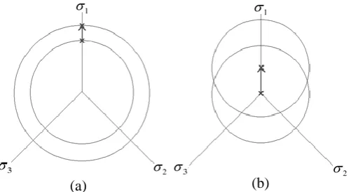
(a)

(b)

Figure 1 – Schematic diagram in stress space showing the behaviour due to (a). Isotropic hardening and (b). Kinematic hardening.

During strain range controlled isothermal cyclic loading tests (such as those considered later in this paper), several different long term responses can be observed if specimens are taken to failure. The stress range (Δσ, defined as half the difference between the maximum and minimum stresses in a cycle, found at the end of tensile and compressive loading regions, respectively) will evolve as load cycles are applied (Figure 2). The specific response depends greatly on the type of material tested. A P91 steel is used in the present work and its behaviour is described here. P91 will exhibit primary cyclic softening (an initial non-linear behaviour

characterised by a monotonic decrease in the stress range reduction rate [6]), followed by a stabilised secondary region with constant rate of change in the stress range [7] (see Figure 2). Ultimately, damage will accumulate in specimens leading to failure, which is clearly characterised in Figure 2 by the reduction in stress range (tertiary behaviour).

Figure 2 - Experimental stress range evolution for isothermal cycle testing (using strain limits of ±0.5% and a 2 minute hold period) at 600°C till specimen failure.

Optimisation procedures offer a method to fine tune constants for material models based on initial estimates (which may be derived based on critical assumptions). The practical employment of optimisation procedures can be difficult however due to, in part, experimental scatter in data. Difficulties arising from this factor are

discussed; with potential solutions offered and demonstrated in examples.

2. The Chaboche Unified Visco-Plasticity Model

The Chaboche model decomposes total strain into elastic and plastic components, incorporating the evolution of both kinematic and isotropic hardening (or softening), through the use of appropriate stress tensors (in a multiaxial condition). The uniaxial form of the Chaboche model is used to illustrate the optimisation procedure described in this paper. Therefore a brief description of the Chaboche model is given.

0

f



 

   

R k

Only elastic behaviour will occur when the value of this function is less than or equal to 0. The back stress (χ) designates the centre of a yield surface and the drag stress (R) denotes the variation of its size from its initial size, k [1]. The constant k should not be confused with the tensile yield stress of a material. In strain controlled experimental results, k is usually taken to be the stress at which in-elastic behaviour is first observed in the first full tensile loading branch of the first cycle. While initial values of k may be similar to the tensile yield stress, optimised values have been commonly found to be significantly less. Note drag stress can either act to increase or decrease the size of the yield surface [1]. Through the use of these quantities, kinematic and isotropic hardening, respectively, may be represented. The term |σ-χ| allows for the interpretation of the absolute distance between the loading point and the centre of the yield surface in stress space. For equation 2.1 therefore, it can be seen that when f has a value less than or equal to 0, the stress point (σ) must lie within the yield surface,

indicating elastic deformation only.

To provide a better approximation of kinematic effects, the back stress can be decomposed into several components [1, 8] (note in the present study, a two back stress component model was found to be satisfactory [3]). An Armstrong and Frederick type kinematic hardening law is used to define the increment for each back stress component, taking the form of equation 2.2 [11].





i i i i

d





C a d







dp

where ai and Ci are both material constants (ai defines a stationary value of the back stress component and Ci dictates how quickly this value is achieved with the increase of plastic strain [11, 12]). The accumulated plastic strain (p), on which most of the internal variables are dependent, is a monotonically increasing quantity and is the summation of the modulus of the plastic components of total inelastic strain (εp), or described

mathematically in equation 2.3 [3].

p

dp



d



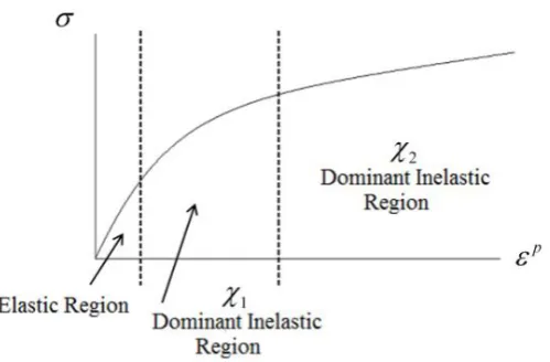
By decomposing the back stress into multiple components, transient and long term behaviour may be accounted for [13], here with a1 and C1 dictating the evolution of χ1 (which describes initial kinematic non-linearity) and a2 and C2 dictating the evolution of χ2 (describing asymptotic, stabalised behaviour), see Figure 3. The total back stress is given as the summation of these components; therefore for m components of back stress, the total back stress (χ) is given by equation 2.4. In the present work, 2 back stress components have been found to be sufficient to describe the material tested (P91). Additional back stress components can aid in the description of non-linear kinematic hardening behaviour. Components will be dominant in certain hardening regions and recessive in others. The use of multiple back stress components is of particular importance when describing non-linear kinematic behaviour that cannot be adequately represented by a single Armstrong-Frederick expression.

1

m

i i











The effects of isotropic hardening (or softening) are represented by the scalar drag stress (R). As such, R will alter only the size of the yield surface; it’s evolution controlled by equation 2.5 [1]. Note that, with the drag stress differential in this form, only primary behaviour (either hardening or softening) can be represented (see Figure 3). Modifications exist to extend the applicability of the Chaboche model to the secondary behaviour region [14], however this is considered outside the scope this paper. The drag stress will undergo some initial monotonic increase before reaching a stabilised asymptotic value [3, 11, 12] (see Figure 4). This saturated value is signified by Q, with the rate at which the stabilised value is reached being determined by the material constant

b, see equation 2.5 [3].





dR



b Q R dp



stress, summarised by equation 2.6 [11, 12], where the scalar components of stress act to increase or decrease the size of the yield surface around its centre (defined by the back stress, χ):

(

R

k

) sgn(

)









 



 



where the function sgn(x) is defined by equation 2.7.

1

0

sgn( )

0

0

1

0

x

x

x

x









_



 



2.7

The viscous stress is assumed to take the form of a power law [1], such as equation 2.8.

1/n

v

Z p





where Z and n are viscous material coefficients. Recalling the definition of the flow rule, paying particular attention to the condition of normality (applicable for the study of metals [15]), equation 2.9 may be applied. Note here n defines the normal direction.

3

2

p

d

d

f

d

n

dt

dt

dt



 









Although not relevant in the uniaxial condition, where the action of the normality rule is easily comprehended, it is worth pointing out that the direction of plastic strain increments must be considered in the deviatoric space for multiaxial loading to represent the translation of the von Mises cylinder [1, 15]. The direction of translation, which is normal in the plane, can be given, in general, by the difference between of the deviatoric components of the total stress and the back stress.

The uniaxial plastic strain increment is given by application of the flow rule (equation 2.9), shown in equation 2.10. Note this is a simplification of the multiaxial form, with tensorial terms such as σ and χ being redefined to scalar ones [2]. Note that the definition of the brackets used in equation 2.10 is given in equation 2.11.





sgn

n

p

R k

d

dt

Z

 





  

 



0

0

0

x x

x

x





 

_

Figure 3 - Evolution of back stress in stress/strain space and illustration of the regions of dominant components.

Figure 4 - Evolution of drag stress (shown for a material undergoing primary hardening).

3. Optimisation of Material Parameters 3.1 Optimisation Procedure

The need for optimisation procedures in determining material constant values that will result in good fits to experimental data is vital when implementing the Chaboche model. The procedure for determining initial estimates of the material constants is detailed elsewhere [3, 11, 13] and will not be repeated here. The need for optimisation stems from the assumptions made (e.g. by Tong et al. [11]) when estimating initial values for the material constants, namely:

- Initially, all hardening is assumed to be isotropic (the kinematic state variable are assumed to be zero), allowing for the saturation value Q to be determined (see Figure 4). The remaining isotropic hardening parameter (b) is found by considering the variation of Δσ before saturation.

- When estimating kinematic hardening constants, it is assumed (for the integration of the related differential equations, see Tong et al [11]) that the viscous stress (σv) remains constant, but in reality this may not be the case.

- It is assumed that the contribution of χ1is negligible in the latter stages of kinematic hardening (see Figure 3). The effects of χ2 may therefore be isolated and applied only to the later stages of hardening.

- Commonly, initial estimates of the visco-plastic material constants (Z and n) are approximated by trial and error or taken from literature to provide a reasonable fit to the stress relaxation regions [3].

relative fitting quality of a given set of coefficients (relating to a function which describes the experimental data) [16, 17]. This can be expressed in terms of N objective functions by equation 3.1.

1

( )

( )

min

N

j j

j

F x

w F x









In general, an objective function (Fj(x)) takes the form of equation 3.2.





( )

( )

j

M

pre

j ij ij

i

F x

A x

A









where x is a real set of, say, n variables that are to be optimised. Side constraints in the form of upper and lower limits (UB and LB respectively) for each of the variables to be optimised are specified [17]. It is necessary to restrict the optimisation space in this way in order to make optimisation procedures timely and to ensure material constant values determined will be in a physically relevant range. For an n-dimensional x vector of material constants, equations 3.3 and 3.4 are true.

n

x 3.3

LB x UB 3.4

For the jth objective function, a weighting value (wj) is applied, ensuring that contributions from different data sources are kept comparable (equation 3.5) [16].

exp

max

N

j j j

j ij

M

w

M

A





where Mj indicates the number of data points for the jth objective function (for N sources of data) and max|Aijexp| is the maximum experimental value from the data source associated with that objective function. The quantity

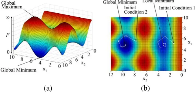
A(x)ijpre represents a specific (the ith) predicted value of some quantity of interest that is considered by the specific objective function, while Aijexp represents the corresponding experimental value. To illustrate the general behaviour of optimisation procedures, consider a two dimensional optimisation problem (see Figure 5 (a), and note that the function chosen to calculate the objective function has no relation to the Chaboche model, but was chosen to give suitable variations to graphically illustrate the potential problems encountered in gradient based optimisation procedures). A range of values for the parameters to be optimised (in Figure 5 (b) these are deemed

x1 and x2) are plotted in the x-y plane, with the value of a single objective function (F) plotted in the z axis. A global minimum is noticed at x1≈4.5 and x2≈9.5. It can be seen from Figure 5 (b) that if the initial conditions are good (in the vicinity of the global minimum), a gradient based optimisation procedure (such as the Gauss-Newton method [16] implemented later through the MATLAB function LSQNONLIN [18]) will produce iterative solutions that will converge on it. If however initial conditions are not close enough to the global minimum or are separated by some “topographical” feature, convergence may be to a local minimum. Another potential pitfall arises when considering combinations of constant values that, when applied to the objective function (or functions used to calculate it, as in the Chaboche model), results in physically unrealistic values. For example, for some functions, a certain combination of constants could lead to the result of an infinite value. It is, obviously, impossible to gauge this against the reference value, and hence the optimisation would fail due to the inability in evaluating the objective functions. These potential problems highlight the vital importance of representative initial conditions (with sensible boundary conditions) and makes it clear that the complexity of this problem increases when more dimensions are added.

It is worth commenting on the use of gradient based methods in optimisation procedures. As identified previously, optimising along the path of greatest descent potentially leads to solutions converging on local (rather than the desired global) minimums. Indeed, in the present work (remembering the highly

material constants is well-established however, and it is assumed that these values are in the vicinity of the global minimum. The act of optimisation only attempts to “fine tune” these initial values. If the use of gradient based methods does converge on a local minimum therefore, it is likely that it will too be in the vicinity of the global minimum.

The use of gradient based methods also has some practical advantages over alternative optimisation methods (such as evolutionary or genetic algorithms [19] and neural networks [20]). Gradient based methods are usually far easier to program and require a great deal less computational effort (binary genetic algorithms are known to be highly computationally expensive [19]). The pattern search aspect of an evolutionary algorithm requires many individual’s “fitness” to be evaluated. This may be done relatively quickly for creep models [19], where ODE evaluation is required for a relatively small number of data points. On the other hand, many cycles of data are used to optimise the material constants of unified visco-plasticity models, greatly lengthening the procedure. As such, the more direct gradient based methods tend to complete in a practically manageable time period. With a more adaptive material model (i.e. on that can accommodate the effects of temperature or strain rate), higher levels of constraint can be imposed on the optimisation by using multiple sources of experimental data (this will be the focus of future publications). This should assist in a solution converging on a global minimum.

(a)

(b)

Figure 5 – (a) Example of global minimum and maximum in a 2 dimensional optimisation problem, illustrating the variation in objective function value. (b) Illustration of convergence on minima of the objective function (indicated by blue shades in the contour plot) for different initial conditions, using a Jacobi matrix to determine

iteration conditions.

3.2 Objective Functions

In total, three objective functions were defined to obtain fits to experimental data. By using multiple objective functions, preference can be given to areas of key interest in the stress-time profile (such as peak stress values) while overall fitting is still accounted for elsewhere.

Fundamentally, the experimental data can be considered as a pair of curves or profiles (stress versus time and strain versus time) where, in this paper, the strain profile controls the stress curve (i.e. strain profiles were used in experiments to load specimens, with resulting variations in stress being recorded). Experimental strain and time increments are used in conjunction with the Chaboche differential equations (for a specific set of material constants that is to be evaluated) to determine predicted stress values. Clearly, the predicted and experimental stress values will occur at the same point in time, meaning that they can be directly compared. Note that after optimisation, the Chaboche model can be used, with the optimised material constants and uniform time and strain increments (kept comparable to the experimental data) to give smoothed output data, allowing for easier comparison to the experimental results.

General stress fitting is accounted for in the first objective function (equation 3.6).





( )

( )

F x



x











where each experimental stress value (σiexp) is compared to the corresponding predicted stress value (σ(x)ipre). This is completed for all selected experimental data points (M1). It is particularly important that the optimisation considers the hardening/softening behaviour of the material through the change in stress range with loading (see Figure 2), as this represents the general evolution of the yield surface and yield stress of the material. Stress range fitting must therefore be applied. This can be found from taking the difference between the peak stresses (found at the end of the tensile branch) and the minimum stresses (found at the end of the compressive branch) and dividing by two for each cycle in turn, for both predicted (Δσ(x)i

pre

) and experimental (Δσi exp

) results, see equation 3.7. The value of M2 will be equal to the number of cycles considered.





( )

( )

F x



x











 

Finally, the stress relaxation (or strain hold) branch is of particular importance as it represents a period of creep dominant behaviour within the model. An objective function that represents this region will therefore aid in the determination of the viscous stress material constants (Z and n, see equation 2.8). Stress values predicted in the relaxation section (σ(x)i-RELAXpre) are compared to corresponding experimental values (σi-RELAXexp) in an additional objective function (equation 3.8).





( )

( )

i RELAX i RELAX

i

F x



x











3.3 Experimental Data Cleaning 3.3.1 Requirements

Experimental data will, unavoidably, include scatter. In the domain of cyclic hardening, this may be due to fluctuations in temperature within the test chamber or due to fluctuations in strain rate. Also, inertial effects will cause the test machine to potentially slightly overshoot the maximum or minimum limit strains. Due to the large amounts of data generated, it is of critical importance that as much of the handling process is as automated as possible.

Different logic conditions are used, in turn, to determine the end of each of the loading branches. Scatter can however result in incorrect points being selected as the branch ends. Consider the case where an experimental point midway in the relaxation region is erroneously selected as the beginning of the compressive branch due to data scatter. From the programs perspective, a subsequent point would be expected to have a lower strain value due to the reverse loading in the compressive branch, however this may well not be the case as a result of the incorrect branch definition (the points being compared are actually both in the relaxation branch, rather than at the beginning of the compressive branch). If a positive strain increment is calculated where a negative one is expected, the related time increment (found through use of the test strain rate) would be negative, hence causing the differential equation solver to fail.

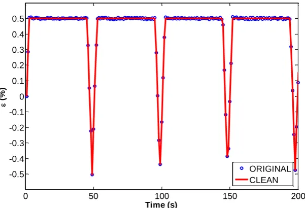
cyclic loops from the strain rate and strain limits. An example of the effects of the cleaning procedure on the strain versus time profile can be seen in Figure 6.

0 50 100 150 200

-0.5 -0.4 -0.3 -0.2 -0.1 0 0.1 0.2 0.3 0.4 0.5

Time (s)



(

%

)

ORIGINAL CLEAN

Figure 6 - Example of the effect of cleaning on the strain profile (note maximum strain is held over hold period in cleaned data).

3.3.2 Effects Compared to Unclean Data

Given the manipulation of the experimental data, it is of paramount importance that no corruption should take place that would otherwise cause unsatisfactory fitting after optimisation. An investigation was therefore conducted on the comparative performance between the use of cleaned and un-cleaned experimental data using the Chaboche model. Using isothermal (600°C) experimental data for a P91 steel, with a strain limit range of ±0.5%, a strain rate of 0.1%/s and a hold time of 2 minutes, optimisation by the two different methods was performed. In the optimisation methods, both cleaned and un-cleaned data were used on the first 49 cycles. Additionally, to illustrate the benefit of the robustness the cleaning procedure can offer, an optimisation procedure was conducted on a greater number of cycles (122) of the cleaned data. Due to the scatter, this number of cycles could not be considered in the optimisation procedure for un-cleaned data. Note that in all cases, the same initial conditions were used (see Table 1).

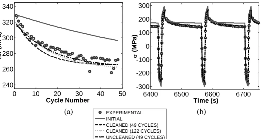
The prediction of the change in stress range during cyclic softening (or hardening) is of importance for industrial applications due to its relation to the change in yield stress of the material (with progressive cycling) and its non-linear nature. The prediction of the changes in stress range for 49 cycles is given in Figure 7 (a), for all three optimisation scenarios. All three optimisation methods give reasonably good approximations of the variations in stress range whether scatter in the experimental data is considered or not.

In addition to the stress range prediction, specific stress magnitude predictions within cycles are also required. To illustrate this, the fitting of the penultimate cycle is provided in Figure 7 (b). It can be seen that, generally, all of the methods give excellent estimation of the stresses generated during tensile, stress relaxation and

compressive branches. The operation of cleaning the data prior to optimisation has not impaired the quality of the overall fit to experimental data. Cleaning will mean automated analysis can be made more robust and will avoid unexpected errors due to incorrect branch definition. For subsequent sections of this paper, the data used will have undergone cleaning first to remove scatter in the strain hold period.

0

10

20

30

40

50

240

260

280

300

320

340

Cycle Number





(

M

P

a

)

6400

6500

6600

6700

-300

-200

-100

0

100

200

300

Time (s)



(

M

P

a

)

EXPERIMENTAL INITIAL

CLEANED (49 CYCLES) CLEANED (122 CYCLES) UNCLEANED (49 CYCLES)

(a)

(b)

Figure 7 – Fitting of (a) stress range variation (indicating primary softening behaviour) and (b) stress values for the final (49th) cycle, by various methods based on an optimisation performed for 49 cycles of P91 data at

600°C.

Table 1 - Material constant values for the original Chaboche model for P91 data at 600 °C using various optimisation methods.

a1 (MPa)

C1 a2 (MPa)

C2 Z (MPa.s1/n)

n b Q (MPa)

k (MPa)

E (MPa) Initial _{52.20 2060.00 67.30 463.00 1750.00 2.70 1.00 -75.40 85.0 1.39E+05}

Un-Cleaned

(49 Cycles) _{73.30 1170.00 49.50 136.00 463.00 9.58 4.23 -57.90 0.51 1.60E+05}

Cleaned (49

Cycles) _{54.60 1080.00 39.90 219.00 501.00 9.70 7.03 -59.40 0.48 1.44E+05}

Cleaned (122

Cycles) 40.00 1280.00 44.30 242.00 477.00 11.20 4.87 -65.80 0.49 1.33E+05

4. Investigation into Performance of Optimisation Program 4.1 Effects of Number of Data Points Chosen per Cycle

By using a greater number of selected experimental data points per cycle, it is expected that the fitting quality of the cyclic stress and relaxation stress values would be marginally improved (given that selected data is

distributed between the beginning and the end of the loading branches). Increasing the number of points selected will increase the number of times that differential equations are evaluated, thus increasing the required

computational effort. Therefore, if optimisation procedures are to be used in practice, an assessment of the minimum number of points that are required for a reasonable fit to the data must be made.

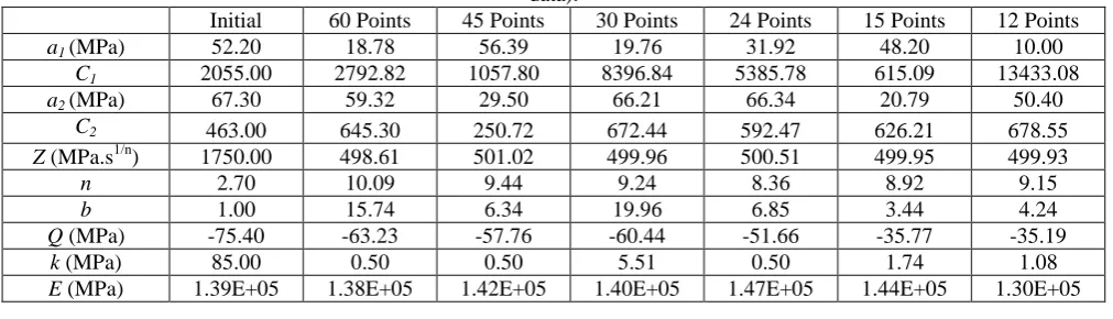
The effect on processing time can be seen in Figure 8, and a summary of the effects that the different number of points selected has on optimised constant values is presented in Table 2. From Figure 8, it is interesting to note that, while in general an increase in the number of points selected per cycle gives rise to an increase in

processing time (as expected), reducing the number of points below approximately 24 points per cycle also has the effect of increasing processing time. As the objective function is formulated by comparing the experimental and theoretical values at these points, a reduction in the number of points considered translates to less available information for the fitting quality to be evaluated by (reduced constraint). It is suspected therefore that, should the objective function tolerance criterion be taken as the preferred termination criterion, a greater number of optimisation iterations may be required in order to give a suitable reduction in the residual value, hence causing an increase in the computing time.

Figure 8 - Processing time (minutes) versus number of points selected per branch (based on an investigation using 49 cycles of data for experiments on a P91 steel at 600°C).

Table 2 - Summary of optimised constants for different numbers of points per cycle (for a P91 steel at 600°C data).

Initial 60 Points 45 Points 30 Points 24 Points 15 Points 12 Points

a1(MPa) 52.20 18.78 56.39 19.76 31.92 48.20 10.00

C1 2055.00 2792.82 1057.80 8396.84 5385.78 615.09 13433.08

a2(MPa) 67.30 59.32 29.50 66.21 66.34 20.79 50.40

C2 463.00 645.30 250.72 672.44 592.47 626.21 678.55

Z (MPa.s1/n) 1750.00 498.61 501.02 499.96 500.51 499.95 499.93

n 2.70 10.09 9.44 9.24 8.36 8.92 9.15

b 1.00 15.74 6.34 19.96 6.85 3.44 4.24

Q (MPa) -75.40 -63.23 -57.76 -60.44 -51.66 -35.77 -35.19

k (MPa) 85.00 0.50 0.50 5.51 0.50 1.74 1.08

E (MPa) 1.39E+05 1.38E+05 1.42E+05 1.40E+05 1.47E+05 1.44E+05 1.30E+05

4.2 Variation of Initial Conditions

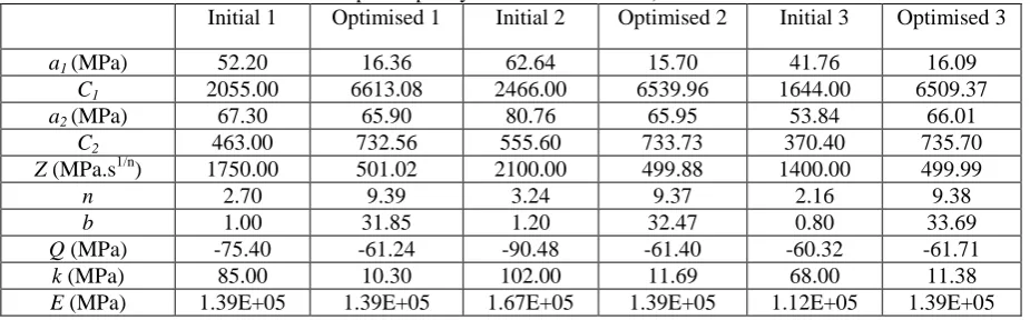
Data for 30 cycles for P91 steel at 600°C was used with the same initial “base” conditions as in section 4.2. A summary of the results of this study is presented in Table 3. An excellent level of agreement was found between constants optimised from the different initial conditions, with an average percentage difference between the base condition case (case 1) and the varied initial condition cases (case 2 for increased initial conditions and case 3 for reduced initial conditions) of approximately 1.2% in both scenarios. A peak percentage different of 13.5% was observed in the initial yield stress (k) value for case 2. Table 4 summarises the percentage differences between optimised material constant sets.

Table 3 - Summary of optimised constants based on different initial conditions (using 30 cycles of data, 30 points per cycle for P91 at 600°C).

Initial 1 Optimised 1 Initial 2 Optimised 2 Initial 3 Optimised 3

a1(MPa) 52.20 16.36 62.64 15.70 41.76 16.09

C1 2055.00 6613.08 2466.00 6539.96 1644.00 6509.37

a2(MPa) 67.30 65.90 80.76 65.95 53.84 66.01

C2 463.00 732.56 555.60 733.73 370.40 735.70

Z (MPa.s1/n) 1750.00 501.02 2100.00 499.88 1400.00 499.99

n 2.70 9.39 3.24 9.37 2.16 9.38

b 1.00 31.85 1.20 32.47 0.80 33.69

Q (MPa) -75.40 -61.24 -90.48 -61.40 -60.32 -61.71

k (MPa) 85.00 10.30 102.00 11.69 68.00 11.38

E (MPa) 1.39E+05 1.39E+05 1.67E+05 1.39E+05 1.12E+05 1.39E+05

Table 4 - Percentage difference between “base” optimised constants (case 1) and varied optimised constants (cases 2 and 3) (using 30 cycles of data, 30 points per cycle for P91 at 600°C).

Percentage difference between optimised 2 and optimised 1

Percentage difference between optimised 3 and optimised 1

a1(MPa) 4.03 1.65

C1 1.11 1.57

a2(MPa) -0.08 -0.17

C2 -0.16 -0.43

Z (MPa.s1/n) 0.024 0.002

n 0.21 0.11

b -1.95 -5.78

Q (MPa) -0.26 -0.77

k (MPa) -13.50 -10.49

E (MPa) 0.00 0.00

5. Behaviour of P91 Steel at 600°C

Experimental data was generated, using an Instron 8862 thermo-mechanical fatigue (TMF) machine. Temperature control is achieved by radio-frequency (RF) induction heating and forced air cooling (delivered through the centre of the specimen). The P91 experimental data presented and analysed in the present work includes isothermal strain controlled cycling tests having a saw tooth strain profile, with strain limits set to ±0.5% and with a 2 minute strain hold period at the end of the tensile branches. Temperature uniformity of the specimen gauge section was such that the entire gauge section was within ±10°C of the testing temperature. Typical experimental variations in gauge length temperature are within ±1°C. Thermocouples were placed along the gauge section, allowing the axial and circumferential temperature gradients to be monitored. The

experimental stress range versus cycle number curve from an isothermal test performed at 600°C is shown in Figure 2, with cyclic softening behaviour being observed [6, 21].

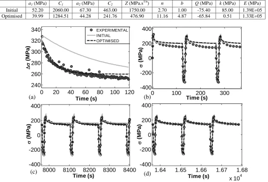
Table 5 - Summary of initial estimates and optimised material constants for the Chaboche model, describing P91 at 600 °C and using 120 cycles of data.

a1 (MPa) C1 a2 (MPa) C2 Z (MPa.s 1/n

) n b Q (MPa) k (MPa) E (MPa) Initial 52.20 2060.00 67.30 463.00 1750.00 2.70 1.00 -75.40 85.00 1.39E+05 Optimised 39.99 1284.51 44.28 241.76 476.90 11.16 4.87 -65.84 0.51 1.33E+05

0

20

40

60

80

100 120

240

260

280

300

320

340

Time (s)





(

M

P

a

)

0

100

200

300

-400

-200

0

200

400

Time (s)



(

M

P

a

)

8000

8100

8200

8300

8400

-400

-200

0

200

400

Time (s)



(

M

P

a

)

1.64

1.65

1.66

1.67

1.68

x 10

-400

-200

0

200

400

Time (s)



(

M

P

a

)

(a)

(b)

(c)

_(d)

Figure 9 – Results of optimisation using 3 objective functions and the Chaboche model for a P91 steel at 600°C (based on 120 cycles of experimental data) showing fitting of (a) stress range, (b) stress values for the first

cycles, (c) stress values for the middle (60th) cycles and (d) stress values for the final cycles.

6. Discussion

The Chaboche model has been implemented in an optimisation procedure using MATLAB [22]. Initial estimates of material constants can be determined from experimental data by making several key assumptions [3]. A reasonable fit to the experimental data can be achieved using these estimates. However, the fitting can be greatly improved using suitable objective functions to compare predicted and experimental data in an optimisation procedure (coefficients of determination increased from 0.9841 to 0.9962 after optimisation for the case considered). The addition of a data cleaning procedure prior to optimisation greatly aids the entire process and makes automated data handling more robust and reliable (as the formation of the objective function relies on accurate dissection of the stress versus time profile). Stress relaxation, which occurs during strain hold periods, can be predicted with far greater accuracy when material constants are optimised using cleaned data (compared to material constants optimised using as received data with experimental scatter). The effect of cleaning on fitting has been assessed against un-cleaned data to verify that cleaning the experimental data has no detrimental effect on the fitting quality.

A reduction in the number of points selected per cycle has been shown to give a reduction in the length required for optimisation up to approximately 24 data points per cycle. The increase in data points necessitates a greater number of times at which the differential equations need to be evaluated, thus requiring a more lengthy

function value, such that a user defined tolerance is exceeded and the optimisation procedure terminates. The optimised constants shown in section 4.2 (Table 2) exhibit a range of values, seemingly dependent on the number of data points selected per cycle. Scatter in the experimental stress data could, when the selection procedure is applied, lead to multiple (slightly different) optimum experimental stress versus time profiles, depending on the specific points selected and rejected. Therefore constants governing the hardening or softening behaviour (such as a1, C1, a2, and C2) could show wide variance as a result of slightly different experimental hardening curves (the tensile and compressive branches) being used for the optimisation, depending on the experimental data points chosen. By comparison, viscous stress constants (Z and n) show remarkable agreement considering the variations which occur in the other values, possibly indicating that stress scatter in the stress relaxation branches (where creep is the dominant mechanism) is far less than that in the hardening data. The selection procedure implemented will always select stress values at the beginning and end of the branches (for use in stress range fitting). At a glance therefore it would be expected that isotropic hardening parameters (b and

Q) would be consistent, regardless of the number of points selected. However in practice, as illustrated in section 2.3, while in the long term hardening effects will be dominated by isotropic behaviour, initially

kinematic effects also may play a key role [8]. Variations therefore in one set of parameters will have inevitable effects on the optimised values of the others. Given some uniform variation, fluctuations in initial condition values do not appear to have an effect on optimised material constant values for a specific optimisation procedure on a given experimental data set.

Optimised constants were used in the prediction of the response of a P91 steel, assuming strain controlled cyclic loading with a hold period to allow for stress relaxation. The stress range is well predicted, as shown in Figure 9, with general stress fitting at specific times being excellent, showing a marked improvement over the initial estimates. Generally, stress relaxation branches are better predicted using the optimised material constants rather than the initial estimates (Figure 9 (c) and (d)), however the stress relaxation in the first cycles of data (Figure 9 (b)) is not accurately predicted by either set. The difficulties in predicting creep behaviour for cyclically loaded specimens have been noted previous by Tong and Vermeulen [13] Zhan and Tong [12, 23]; who suggested that the poor creep prediction may be due to neglecting static/time recovery effects in the Chaboche model [13]. A modification (applied to the kinematic hardening law) was suggested that appeared to address this deficiency [10, 23], however this explanation does not suggest why creep behaviour is well predicted in later cycles in this case. Potentially, the viscous stress term is sufficient to describe the creep response for the hold period

considered in these experiments, however the material has undergone microstructural changes after cycling, therefore the creep response for the first and last cycle cannot be explained by a single set of material constants. A compromise is made in the optimisation procedure to accurately predict the greatest number of stress

relaxation branches, thus sacrificing the quality of the fit of the stress relaxation branches for the initial cycles. Future work will look to address these discrepancies. A divergence can be seen in the stress range prediction (Figure 9 (a)) around the middle of the considered cycle range (approximately 70 cycles). It is possible that the 120 cycles of data used for optimisation in this case comprises of the primary non-linear region and some of the secondary linear region of the stress range profile (see Figure 2).

A source of error that could contribute to discrepancies in stress fitting was proposed by Lin et al. [24, 25] and relates to the cyclic specimen design. It is assumed that the “uniaxial” bar specimens used in cyclic testing are subject to uniaxial stress and strain fields, however this may not be the case. Ridges for the extensometer arms and bending radii at the top of the specimen, together with a short specimen length (used to avoid buckling in reverse loading) have been shown to cause constraint in the specimen which induces multiaxial stress and strain fields [24, 25]. Actual strain levels in regions of the specimen may be ±20% [24] of the value inferred from the extensometer. This phenomenon would cause localised hardening, distorting the stress readings as a result. Such effects should be considered when analysing the fitting quality of results from optimisation procedures.

7. Conclusions

The Chaboche model has the ability to accurately predict the initial non-linear response of a material undergoing isothermal cyclic loading. The predictive capability of the model can be significantly enhanced through the use of an optimisation procedure, which in turn can be aided and made more robust by subjecting experimental data to a cleaning procedure prior to the application of the optimisation process. With this taken into account, fitting is greatly improved and the optimisation procedure can be automated with far more confidence. Using a method to estimate initial values of the material constants for P91 material data at 600°C (subjected to strain controlled cycling of ±0.5%, with 2 minute hold periods at 0.5%), good estimations of the stress response can be obtained. The coefficient of determination (r2) provides a metric with which to gauge fitting quality [16] (in this case comparing experimental results to values predicted by the Chaboche model) and was found to increase from 0.9841 based on the fitting for initial estimates of the material constants to 0.9962 for the optimised values. Future work will focus on the improvement of the fitting, particularly in the prediction of the stress range for materials that do not respond in the same manner as P91, as well as the prediction of the tertiary behaviour region leading to failure, generally thought of to be due to the formation of cavitation damage and cracks [6, 21]. Alternatives to the optimisation procedure or general methodology used will also be analysed. The effects of variations in the viscous law material constants (Z and n) will also be investigated; with a view to improving the stress relaxation fitting quality over a wider cycle range.

8. Acknowledgments

The authors greatly appreciate the support of both E.ON and the EPSRC (case study award number

EP/J50211X/1) through funding this work. Thanks are also extended to Mr Tom Bus and Mr Brian Webster for their assistance in the experimental work.

9. References

[1] J. L. Chaboche and G. Rousselier, "On the Plastic and Viscoplastic Constitutive-Equations .1. Rules Developed with Internal Variable Concept," Journal of Pressure Vessel Technology-Transactions of the Asme, vol. 105, pp. 153-158, 1983.

[2] J. L. Chaboche and G. Rousselier, "On the Plastic and Viscoplastic Constitutive-Equations .2. Application of Internal Variable Concepts to the 316 Stainless-Steel," Journal of Pressure Vessel Technology-Transactions of the Asme, vol. 105, pp. 159-164, 1983.

[3] Y. P. Gong, C. J. Hyde, W. Sun, and T. H. Hyde, "Determination of material properties in the

Chaboche unified viscoplasticity model," Proceedings of the Institution of Mechanical Engineers Part L-Journal of Materials-Design and Applications, vol. 224, pp. 19-29, 2010.

[4] C. Maharaj, J. P. Dear, and A. Morris, "A Review of Methods to Estimate Creep Damage in Low-Alloy Steel Power Station Steam Pipes," Strain, vol. 45, pp. 316-331, Aug 2009.

[5] C. J. Hyde, W. Sun, and S. B. Leen, "Cyclic thermo-mechanical material modelling and testing of 316 stainless steel," International Journal of Pressure Vessels and Piping, vol. 87, pp. 365-372, Jun 2010. [6] N. E. Dowling, Mechanical behavior of materials : engineering methods for deformation, fracture, and

fatigue, 3rd ed. Upper Saddle River, N.J.: Pearson/Prentice Hall, 2007.

[7] G. Bernhart, G. Moulinier, O. Brucelle, and D. Delagnes, "High temperature low cycle fatigue behaviour of a martensitic forging tool steel," International Journal of Fatigue, vol. 21, pp. 179-186, Feb 1999.

[8] J. L. Chaboche, "Time-Independent Constitutive Theories for Cyclic Plasticity," International Journal of Plasticity, vol. 2, pp. 149-188, 1986.

[9] Z. Mroz, "On Description of Anisotropic Workhardening," Journal of the Mechanics and Physics of Solids, vol. 15, pp. 163-&, 1967.

[10] J. L. Chaboche, "A review of some plasticity and viscoplasticity constitutive theories," International Journal of Plasticity, vol. 24, pp. 1642-1693, Oct 2008.

[11] J. Tong, J. L. Zhan, and B. Vermeulen, "Modelling of cyclic plasticity and viscoplasticity of a nickel-based alloy using Chaboche constitutive equations," International Journal of Fatigue, vol. 26, pp. 829-837, Aug 2004.

[12] Z. L. Zhan and J. Tong, "A study of cyclic plasticity and viscoplasticity in a new nickel-based superalloy using unified constitutive equations. Part I: Evaluation and determination of material parameters," Mechanics of Materials, vol. 39, pp. 64-72, Jan 2007.

[14] A. A. Saad, W. Sun, T. H. Hyde, and D. W. J. Tanner, "Cyclic softening behaviour of a P91 steel under low cycle fatigue at high temperature," Procedia Engineering, vol. 10, pp. 1103-1108, 2011.

[15] G. E. Dieter, Mechanical metallurgy, 3rd ed. New York: McGraw-Hill, 1986.

[16] S. C. Chapra and R. P. Canale, Numerical methods for engineers, 6th ed. Boston: McGraw-Hill Higher Education, 2010.

[17] P. Venkataraman, Applied optimization with MATLAB programming, 2nd ed. Hoboken, N.J.: John Wiley & Sons, 2009.

[18] "Optimisation Toolbox TM 4 User's Guide," T. M. Inc2008.

[19] B. Li, J. Lin, and X. Yao, "A novel evolutionary algorithm for determining unified creep damage constitutive equations," International Journal of Mechanical Sciences, vol. 44, pp. 987-1002, May 2002.

[20] M. Abendroth and M. Kuna, "Identification of ductile damage and fracture parameters from the small punch test using neural networks," Engineering Fracture Mechanics, vol. 73, pp. 710-725, Apr 2006. [21] R. I. Stephens and H. O. Fuchs, Metal fatigue in engineering, 2nd ed. New York: Wiley, 2001. [22] "Matlab 7 Mathematics," T. M. Inc2008.

[23] Z. L. Zhan and J. Tong, "A study of cyclic plasticity and viscoplasticity in a new nickel-based superalloy using unified constitutive equations. Part II: Simulation of cyclic stress relaxation,"

Mechanics of Materials, vol. 39, pp. 73-80, Jan 2007.

[24] J. Lin, F. P. E. Dunne, and D. R. Hayhurst, "Aspects of Testpiece Design Responsible for Errors in Cyclic Plasticity Experiments," International Journal of Damage Mechanics, vol. 8, pp. 109-137, April 1, 1999 1999.

[25] J. Lin, D. R. Hayhurst, and F. P. E. Dunne, "Errors in creep-cyclic plasticity testing: their quantification and correction for obtaining accurate constitutive equations," International Journal of Mechanical Sciences, vol. 43, pp. 1387-1403, Jun 2001.