The earliest fragmentation in molecular clouds : and its connection to star formation

(1)

AND ITS CONNECTION TO STAR FORMATION

Rowan Johnston Smith

A Thesis Submitted for the Degree of PhD

at the

University of St. Andrews

2010

Full metadata for this item is available in the St Andrews

Digital Research Repository

at:

https://research-repository.st-andrews.ac.uk/

Please use this identifier to cite or link to this item:

http://hdl.handle.net/10023/929

This item is protected by original copyright

(2)

The Earliest Fragmentation in Molecular

Clouds

and its connection to Star Formation

by

Rowan Johnston Smith

Submitted for the degree of Doctor of Philosophy in Astrophysics

(3)

(4)

Declaration

I, Rowan J. Smith, hereby certify that this thesis, which is approximately 30,000 words in

length, has been written by me, that it is the record of work carried out by me and that it has

not been submitted in any previous application for a higher degree.

Date Signature of candidate

I was admitted as a research student in September 2006 and as a candidate for the degree

of PhD in September 2006; the higher study for which this is a record was carried out in the

University of St Andrews between 2006 and 2009.

I hereby certify that the candidate has fulfilled the conditions of the Resolution and

Regula-tions appropriate for the degree of PhD in the University of St Andrews and that the candidate

is qualified to submit this thesis in application for that degree.

(5)

(6)

Copyright Agreement

In submitting this thesis to the University of St Andrews we understand that we are giving

permission for it to be made available for use in accordance with the regulations of the

Uni-versity Library for the time being in force, subject to any copyright vested in the work not

being affected thereby. We also understand that the title and the abstract will be published,

and that a copy of the work may be made and supplied to any bona fide library or research

worker, that my thesis will be electronically accessible for personal or research use unless

ex-empt by award of an embargo as requested below, and that the library has the right to migrate

my thesis into new electronic forms as required to ensure continued access to the thesis. We

have obtained any third-party copyright permissions that may be required in order to allow

such access and migration, or have requested the appropriate embargo below.

The following is an agreed request by candidate and supervisor regarding the electronic

publication of this thesis: Access to Printed copy and electronic publication of thesis through

the University of St Andrews.

(7)

(8)

Abstract

Stars are born from dense cores of gas within molecular clouds. The exact nature of the

connection between these gas cores and the stars they form is an important issue in the field

of star formation. In this thesis I use numerical simulations of molecular clouds to trace the

evolution of cores into stars.

The CLUMPFIND method, commonly used to identify gas structures is tested. I find that

the core boundaries it yields are unreliable, but in spite of this, the same profile is universally

found for the mass function. To facilitate a more robust definition of a core, a modified

clump-find algorithm which uses gravitational potential instead of density is introduced. This allows

the earliest fragmentation in a simulated molecular cloud to be identified. The first bound

cores have a mass function that closely resembles the stellar IMF, but there is a poor

corre-spondence between individual core masses and the stellar masses formed from them. From

this, it is postulated that environmental factors play a significant part in a core’s evolution.

This is particularly true for massive stars, as massive cores are prone to further

fragmenta-tion. In these simulations, massive stars are formed simultaneously with stellar clusters, and

thus the evolution of one can affect the other. In particular, the global collapse of the forming

cluster aids accretion by the precursors of the massive stars. By tracing the evolution of the

massive stars, I find that most of the material accreted by them comes from diffuse gas, rather

(9)

(10)

Publications

The following chapters have been published in Monthly Notices of the Royal Astronomical

Society.

Chapter 5

‘The Structure of Molecular Clouds and the Universality of the Clump Mass Function ’

Smith, R. J., Clark, P. C. & Bonnell, I. A, 2008

MNRAS,391,1091-1099

Chapter 6

‘Fragmentation in Molecular Clouds and its Connection to the IMF’

Smith, R. J., Clark, P. C. & Bonnell, I. A, 2009

MNRAS, 396, 830-841

Chapter 7

‘The Simultaneous Formation of Massive Stars and Stellar Clusters’

Smith, R. J., Longmore, S. & Bonnell, I. A, 2009

(11)

(12)

Acknowledgements

My thanks must first go to my supervisor Ian Bonnell whose remarkable enthusiasm and

cheerfulness in the face of all obstacles have made this PhD a pleasure. I must also thank

my collaborators; Paul Clark who introduced me to CLUMPFIND then helped me pick up the

pieces afterwards, and Steven Longmore who helped me connect my simulations to actual

observations. I would also like to acknowledge SUPA (The Scottish Universities Physics

Al-liance), who funded the computer that the simulations presented here were carried out on. A

huge thank-you also goes to the staff and students of the St-Andrews Astronomy department

who have provided both useful help, and welcome distractions throughout this PhD.

Finally I must thank my family, without whose support and encouragement this would not

have been possible. Thanks go to my mother, Joanne, my brother, Lewis, and a particularly

(13)

(14)

List of Figures

1.1 The IMF found by Chabrier (2002). . . 10

2.1 An illustration of the binary tree. SPH particles are combined hierarchically into nodes which can be substituted for their constituent particles within the gravitational force calculation. . . 21

3.1 The energy spectrum for a turbulent flow in log-log scales, adapted from a graph from Wilcox (1998) . . . 29

3.2 The velocity dispersion from the centre of the SPH distribution once the veloc-ity field has been applied. The dotted line shows the gradient of the velocveloc-ity dispersion whenβ =0.5 in equation 1.1. In the range 0.1< R <0.5 pc the Larson relation is satisfied. . . 33

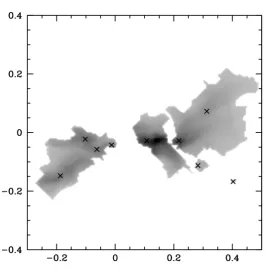
3.3 The positions of a test particle, originally situated at the co-ordinates [0.89 : −0.32]in a uniform flow from left to right with time. . . 34 3.4 The decay of turbulent kinetic energy (in units of initial kinetic energy) in the

absence of driving and self-gravity. . . 35

3.5 The column density after the turbulence has decayed for 1 t_{f f}. The colour scale denotes column densities in the range, 0.001 g cm−2(dark red)to 0.1 g cm−2 (yellow/white). . . 36

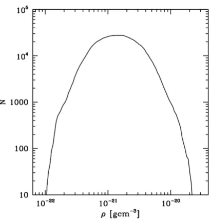
3.6 The PDF of the gas after the turbulence has decayed for 1 t_{f f}. The PDF resem-bles a lognormal as is expected from turbulence in an isothermal gas. . . 36

3.7 The PDF of the gas after 1 t_{f f} when the turbulence was continuously re-imposed throughout its evolution(solid line). When compared to the PDF from decaying turbulence(dotted line)less dense gas had been created. . . 37

3.8 The column density after 1 t_{f f} when the turbulence was continuously re-imposed throughout the evolution. The colour scale denotes column densities in the range, 0.001 g cm−2 (dark red)to 0.1 g cm−2(yellow/white). . . 38

(19)

scheme (solid line). When compared to the PDF from decaying turbulence (dotted line) a greater range of densities have been produced. Note, that N is higher in the driven case merely because this simulation was carried out at higher resolution. . . 40

3.11 The decay of turbulent kinetic energy (in units of the initial kinetic energy) in a collapsing system (solid line). The energy begins to rise again at 1 t_{f f} compared to the case without self-gravity (dotted line when the onset of star formation randomises the velocities. . . 41

3.12 The velocity dispersion from the centre of the molecular cloud as it collapses. The dispersions are shown at 0.25 t_{f f} red, 0.5 t_{f f} green,0.75 t_{f f} blueand 1 t_{f f} black. The dotted line shows the gradient of the velocity dispersion when

β=0.5 in equation 1.1. The velocity dispersion becomes steeper at larger radii due to collapse motions. . . 42

3.13 The PDF of the gas after it has collapsed for 1 t_{f f}. The solid line show the simulation which was initially driven, and the dotted line the simulation which has been allowed to decay. . . 42

4.1 An illustration of the CLUMPFIND algorithm. Four clumps are assigned and they contain material down to the lowest contour. . . 46

4.2 The use of contours to merge and destroy clumps. . . 48

4.3 A cartoon of the potentialclump findingprocess in 1D. For the potential and contours shown, the blue regions contain material which would be assigned to p-cores. . . 50

5.1 The column density of the data file used for the clumpfinding comparison. The density scale is logarithmic and runs from 0.005 gcm−2 (black) to 1 gcm−2 (white). The region shown is 1 pc by 1 pc large and contains 79.5 M. . . 57

5.2 The standard PP clump-find projected in the xy plane, crosses denote the centre of the clumps. This clump-find used data from a 200_×200 grid. The scale is shown in parsecs and the colours represent column densities in the range 0.02 gcm−2 (blue) to 1 gcm−2(yellow) at logarithmic intervals. . . 58

5.3 The intrinsic 3D density profile along the z axes of the material belonging to a typical clump in the standard PP clump-find. About half the material assigned to the clump is truly at high 3D densities but the rest is contamination from material along the line of sight. . . 60

(20)

5.5 Four clumpfinds carried out on the central region where star formation will occur with varying resolution levels.Top leftA 50_×50 grid with a cell width of 4, 125 AU,top righta 100_×100 grid with a cell width of 2, 063 AU,bottom lefta 200×200 grid with a cell width of 1, 031 AU andbottom righta 400×400 grid with a cell width of 516 AU. The scale is shown in parsecs and the grayscale represent column densities in the range 0.02 gcm−2(grey) to 1 gcm−2(black) at logarithmic intervals. Crosses show the centre of the clumps. Note that in some cases a clump will disapear at higher resolution, this is primarily due to the shifting contours meaning that some clumps no longer meet the resolution criteria. . . 63

5.6 The variation of the cumulative number clump mass function with resolution. The clump-finds shown are from thered50×50 grid with a cell width of 4, 125 AU,green100_×100 grid with a cell width of 2, 063 AU, the black200_×200 grid with a cell width of 1, 031 AU and theblue400_×400 grid with a cell width of 516 AU. Error bars depict the uncertainty from Poisson noise. Clumps from each orthogonal projection were included to improve the statistics. . . 64

5.7 The cumulative number clump mass functions found from PP data with three different lower column density limits; solid line0.01 gcm−2, dashed line0.05 gcm−2 anddotted line0.1 gcm−2. Error bars depict the uncertainty from Pois-son noise. . . 65

5.8 Clumpfinds using various data-sets.Top left the standard PP clump-find. Top rightapplied to a data set above an intrinsic 3D density of 104 cm−3. Bottom leftusing the PPV data-set with 16 velocity bins, corresponding to a velocity resolution of 0.33 kms−1. Bottom rightthe 3D clumpfind on the raw SPH data. The scale is shown in parsecs and the grayscale represent column densities in the range 0.02 gcm−2 (grey) to 1 gcm−2 (black) at logarithmic intervals. Crosses show the centre of the clumps. . . 66

5.9 A projection of the real 3D density profile of the clump shown in Fig 5.3 when found using PPV data with 16 velocity bins instead of just PP data. . . 68

5.10 The cumulative number clump mass functions from the previous clumpfinds. Top leftthe standard PP clump-find,top righthigh density PP data,bottom left the PPV clump-find andbottom rightthe PPP (SPH) method. The dashed lines are power law fits whose gradients are shown in Table 5.7. . . 70

6.1 The simulated Giant Molecular Cloud at one dynamical time. The colours rep-resent column densities in the range 0.001gcm−2 (red) to 10 gcm−2 (white). Sink particles are shown as white dots and the cloud is viewed along its long axis. . . 79

(21)

ward from the peak of gravitational potential. There is considerable dispersion due to substructure, but there is a clear trend showing a flattened central peak and density decreasing outwards. . . 84

6.4 Histograms of the masses & sizes of the bound (solid line) and composite (dotted line) p-cores. Panel (a) shows the clump mass function. Masses above 0.2 M are resolved and the Saltpeter slope is denoted by a dashed line. Panel (b) shows the effective radii. Panel (c) shows the best fit values ofnfor the profile

ρ∝ r−n. The p-core mass function resembles the stellar IMF and the p-cores are typically small, centrally concentrated objects. . . 85

6.5 The binding of the composite p-cores. Panel (a) shows a histogram of the energy ratio of the cores, E_{r at} _≥1 are bound, whereE_{r at} =_|E_p_|/E_{ther m}+E_k. Panel (b) shows the p-core masses plotted against energy ratio, blue circles denote cores with a steepn>1.5 density profile, green squares intermediate 1 < n < 1.5 profiles, and red crosses shallow profiles. Panel (c) shows the density exponentnplotted against energy ratio with error bars due to the poor fit from density substructure and non-spherical core shapes; the straight line has a gradient of two. There is no correlation between binding and mass, but there is a link to central concentration. . . 87

6.6 The one dimensional internal velocity dispersions of the p-cores in the bound(solid line) and composite (dotted line) datasets. The sound speed of an isothermal gas at 10K is 0.2 kms−1which means the p-cores are generally subsonic . . . 89

6.7 The cumulative mass functions from snapshots at solid 0.6 t_{d y n}, dotted 0.8

td y n,short dashed1 td y n andlong dashed1.2 td y n. The dot-dashed line shows

the Salpeter slope. The mass function gets steeper with time as the high mass p-cores are formed earlier. . . 90

6.8 The connection between p-core masses at a snapshot in time and their sink mass when the simulation was stopped. The solid line shows a 1-1 correspon-dence. There is a poor correlation between p-core mass and the total sink mass formed from them. . . 91

6.9 The connection between clump mass and sink mass at successive dynamical times. Panel (a) td y n =1, (b) td y n =2, (c) td y n =3, (d) td y n =5. The solid

line shows a 1-1 correspondence. There is now a clear connection between p-core mass and sink mass, but it still shows significant dispersion. . . 93

6.10 The CMF of the p-cores with mass bins denoted by different colours. . . 94

(22)

7.1 The evolution of the centre of clump Alphatop. The snapshots shown are atleft 0.75 t_{d y n} (3.53_×105 yrs),middle1 t_{d y n} (_∼4.7_×105 yrs) andright1.25 t_{d y n} (5.9_×105 yrs) respectively. The colour scale denotes column densities from 0.05 g cm−2to 5 g cm−2. The structure becomes more compact with time, and decreases in substructure. . . 109

7.2 The evolution of the centre of clump Betamiddle. The snapshots shown are at left0.75 t_{d y n} (3.53_×105 yrs),middle1 t_{d y n} (_∼4.7_×105 yrs) andright1.25

t_{d y n} (5.9_×105 yrs) respectively. The colour scale denotes column densities

from 0.05 g cm−2 to 5 g cm−2. The structure becomes more compact with time. 110

7.3 The evolution of the centre of clump Gammabottom. The snapshots shown are atleft0.75 t_{d y n}(3.53_×105yrs),middle1 t_{d y n}(_∼4.7_×105yrs) andright1.25

t_{d y n} (5.9_×105 yrs) respectively. The colour scale denotes column densities

from 0.05 g cm−2 to 5 g cm−2. The structure becomes more compact with time. 111

7.4 The global properties of the mass within 1 pc of the most massive sink for clumps Alpha(solid line), Beta(dotted line)and Gamma(dashed line).Top, the total mass andbottom, the mass weighted dispersion of matter plotted against the simulation dynamical time (t_{d y n}_∼4.7_×105yrs). The clump mass increases with time and becomes more concentrated. . . 112

7.5 The masses and column densities around the central sink in clumps Alphatop, Betamiddleand Gammabottomplotted against the simulation dynamical time

( t_{d y n}_∼4.7_×105yrs). The dashed line shows the sink mass and the solid line

the column density calculated in a 0.15 pc box centered on the sink. . . 114

7.6 The dust continuum emission at 230 GHz from clump Alpha at top 0.75 t_{d y n} (3.53×105yrs), andbottom1.25 t_{d y n}(5.9×105yrs). The colour scale denotes emission from 0.5 mJy (dark blue) to 500 mJy (yellow). As the clump becomes more evolved the emission from its centre, where the massive stars are forming, increases. . . 116

7.7 The observable properties of the mass within 1 pc of the most massive sink calculated from a 2D grid with a size resolution of 0.03 pc, plotted against the simulation dynamical time (t_{d y n} _∼4.7_×105 yrs). The clumps are denoted by the following lines; Alpha(solid line), Beta(dotted line) and Gamma(dashed line). The panels show: top, the total emission from the clump andbottom, the emission weighted dispersion. . . 117

7.8 Simulated interferometry observations of clump Alpha top at the same time intervals as shown in Figure 7.1. . . 119

7.9 Simulated interferometry observations of clump Betamiddleat the same time intervals as shown in Figure 7.2. . . 120

(23)

growth in sink mass over a period of 0.25 t_{d y n} plotted against the average potential in code units of the mass within a pc radius of the sink. The sinks in the deepest potential well grow the most significantly.Bottomthe mass in sinks within regions Alphasolid line, Betadotted lineand Gammadashed lineplotted against their dispersion. The mass in sinks grows as the clump becomes more concentrated. . . 122

7.12 The final fate of the mass within clump Alpha shown at 1 t_{d y n}. The green dots show the positions of gas which will eventually be accreted by the massive sink (red dot). Black dots show the position of sinks and blue dots show the location of material in cores. The gas which will be accreted by the massive sinks is well distributed throughout the clumps, and generally cores within this region will not be disrupted by the massive sink. . . 125

7.13TopThe density distribution of the material which will be accreted by the cen-tral sink in clump A (green), compared to that of the material in cores at

t_{d y n}=1 (blue).BottomThe cumulative density distribution of the entire clump

(24)

List of Tables

1.1 Typical properties of clouds, clumps and cores (adapted from Bergin & Tafalla 2007.) . . . 3

5.1 All the clump-finding presented in this paper were performed on a single SPH simulation. The initial conditions of the simulation are given here. The mass resolution is the minimum mass gravitational forces can be resolved for and is calculated via M_{r es} _∼ 100M_{t ot al}/N_{par t}. The Jeans mass, free-fall time and sound speed are calculated from the average density of the simulation be-fore collapse using the formulae M_J = (4πρ/3)−1/2(5kT/(2Gµ))3/2, t_{f f} =

(3π/(32Gρ))1/2. . . 55 5.2 The parameters used to find the standard PP clumpfind shown in Figure 5.2.

The resolutions grid cells correspond to a physical length of 1, 031 AU. . . 59

5.3 The properties of the clumps found in different orientations. The starred case corresponds to the standard PP clump-find. . . 60

5.4 The recovered clumps at different resolutions for clump-find on PP data in the x-y plane. The * denotes the fiducial case and the resolution is given in grid cells. 62

5.5 The properties of the clumps using the PPV data-set compared to the standard PP clump-find. The 16 velocity bins have a width of 0.33 kms−1 and the 40 velocity bins a width of 0.13 kms−1 . . . 67

5.6 A comparison of the clump-find results. . . 69

5.7 The best fit power law gradients for the cumulative CMF’s shown in Figure 5.10. 71

6.1 Given below are the initial conditions of the simulation analysed in this paper. The mass resolution is the minimum mass gravitational forces can be resolved for and is calculated viaM_{r es}∼100M_{t ot al}/N_{par t}. . . 78

6.2 The average clump properties of the p-cores in the bound and composite datasets.

R_{e f f} is the radius within which 68% of the mass is contained. The density

pro-file is the best fit value of n for the propro-fileρ∝r−n. . . 84

(25)

2007.) . . . 102

7.2 The massive clump properties recorded at the beginning (3.53_×105 yrs) and end (5.9×105yrs) of the analysed period. The first massMis that found within a 1 pc radius of the central sink. The second is that within a cylindrical column of radius 1pc centered on the same sink. The mean gas density is denoted by

¯

ρg, and max. Ms and tot. Ms represent the maximum sink mass within the

clump and the total sink mass respectively. . . 106

(26)

1

Introduction

Since no energy source is inexhaustible, stars cannot exist forever. Instead they are born in

dense nebulae and die in either spectacular supernovae explosions or have a more lingering

death as a planetary nebulae. This thesis will concentrate on the earliest stages of the birth of

stars: their condensation from their parent nebulae.

Considerable work has gone into understanding star formation since the pioneering work

of Jeans (1902), who first derived the criteria for a region of gas to become unstable and

collapse to form a star. We now understand that stars are formed in dense nebulae, known

as molecular clouds. The gas in the region collapses when it becomes gravitationally unstable

and forms a hydrostatic core surrounded by an accretion disk, within which planets may be

formed. The material from this disk is accreted by the actual star, which powers energetic jets.

However, there are many facets of this process as which are as yet unknown. The

distribu-tion of stars formed has a characteristic profile common to all regions of star formadistribu-tion. There

(27)

ther-modynamics, but a definitive answer has not yet been reached. Moreover, the nature of the

link between the dense cores of gas within molecular clouds and the stars which form from

them is still unclear. An additional challenge is understanding massive star formation, since

the typical fragmentation mass within molecular clouds is an order of magnitude smaller than

the largest stars, and feedback from the star could prevent very high masses being reached.

At the level of individual stars the mechanism for transferring angular momentum from the

disk into the jet is still uncertain.

This thesis seeks to address the connection between the earliest self-gravitating fragments

in molecular clouds, and the stars which form from them. Particular emphasis will be placed

on the role of gravity in a clustered environment. In this introduction to the topic I will first

describe the environment of molecular clouds and how they are observed in Section 1.1. Then

in Section 1.2 the major processes in star formation will be outlined. Finally, in Section 1.3

the dense cores which are the progenitors of stars are described, and the similarities between

the clump mass function and the stellar initial mass function discussed.

1.1 The Properties of Molecular Clouds

1.1.1 Observations

Since the first observations by Bok of dark nebulae or ‘Molecular Clouds’, they have been

recognised as the birth places of stars (Bok & Reilly, 1947). Due to the very low densities

of space (typically less than one atom per cubic centimeter), the self-gravity of gas is largely

negligible. It is only in the clouds of gas where large density enhancements are seen that

gravity can become a significant enough force to induce collapse. Molecular clouds are

pre-dominately situated in the spiral arms of our galaxy, and get their name from the molecular

hydrogen which is their chief constituent, although they also contain dust and traces of other

molecular species.

Since the discovery of molecular clouds (MC’s) considerable effort has gone into

deter-mining their properties. This process is complicated by the fact that the main constituent of

MC’s, (molecular hydrogen) is effectively unobservable at low temperatures, due to its lack of

dipole moment. However, several observational methods have been developed which cleverly

get around this obstacle. A fruitful approach is to observe dust within MC’s rather than the

(28)

1.1. The Properties of Molecular Clouds

Table 1.1:Typical properties of clouds, clumps and cores (adapted from Bergin & Tafalla 2007.)

Cloud Clump Core

Size (pc) 2−15 0.3−3 0.03−0.2

Mass (M) 103₋104 50₋500 0.5₋5

Mean density (cm−3) 50₋500 103₋104 104₋105 Velocity Extent (kms−1) 2−5 0.3−3 0.1−0.3

Gas Temperature (K) _∼10 10₋20 8₋12

the mean observed value of 100 is used as the gas to dust ratio, however Lilley (1955) found

a range of values between 35 to 250, therefore this assumption is likely to introduce at least

some error. The peak in thermal emission from dust particles is situated in the sub-mm regime

allowing the dust continuum to be mapped using mm bolometer arrays such as SCUBA and

MAMBO (e.g. Motte et al., 1998; Johnstone et al., 2000; Enoch et al., 2006). Another method

which uses the dust component is extinction mapping. This takes advantage of the fact that

the dust absorbs optical and near-IR light from the background stars. By measuring the colour

excess of the background the extinction can be deduced, since short wavelengths will be

pref-erentially absorbed. This is known as the Near Infrared Colour Excess (NICE) method (Lada

et al., 1994), and also comes in an improved NICER (NICE Revisited) variant (Lombardi &

Alves, 2001).

Alternatively, line emission from one of many trace molecular species can be used to trace

the gas. Carbon monoxide and its isotopologues are commonly used tracers of the more

diffuse gas (Pineda et al., 2008) but as CO freezes out onto dust grains above densities of

3_×104 g cm−3, nitrogen bearing molecules such as NH₃ are used to trace the dense regions.

1.1.2 Structure and Velocity Distribution

Molecular Cloud structure appears clumpy and filamentary (Williams et al., 2000), and in

many ways its hierarchical structure appears scale free, which has lead some authors to use

fractal models to describe it (e.g. Elmegreen, 2002). However, it is more common

observa-tionally to split the structure up into ‘clouds’, ‘clumps’ and ‘cores’, which can be defined as

shown in Table 7.1 by Williams et al. (2000). These approaches are not incompatible:

ef-fectively clumps and cores are equivalent to the high density peaks of a fractal distribution.

Unfortunately making these divisions can often be quite arbitrary.

Most of the mass in molecular clouds actually resides at low densities, for example

(29)

Pipe Nebula hasAk>10. Similarly, in continuum emission from Ophiuchus, Johnstone et al.

(2004) found that sub-millimetre objects represented only 2.5% of the cloud mass. Indeed,

Table 7.1 shows that the range of gas densities seen in Molecular Clouds is extremely wide.

Gas densities are well described by a lognormal distribution (e.g. Ridge et al., 2006), which

is a characteristic of structure formed by turbulence in an adiabatic gas (Vazquez-Semadeni,

1994; Scalo et al., 1998).

Supersonic linewidths observed from Molecular Clouds have long been interpreted as

ev-idence for said turbulence. These were described by Larson (1981) who related the velocity

dispersionσ(v)of a cloud to its size Las shown in Equation 1.1

σ(v)_∝Lβ (1.1)

where a value of β _≈ 0.4_±0.1 is typically observed. Larson (1981) developed this

rela-tion by analogy to classical subsonic Kolmogorov turbulence, but turbulence in MC’s actually

has a closer resemblance to Burgers turbulence (Brunt & Mac Low, 2004). Burgers

turbu-lence is supersonic, compressible and most of its energy is dissipated by shocks, which causes

large density enhancements. In an isothermal gas the density across a shock increases as the

square of the Mach number, and therefore as Mach numbers of up to 10 are observed,

den-sity enhancements of at least two orders of magnitude are obtainable. This mechanism could

produce the cores discussed above. However, as Ballesteros-Paredes (2004) point out, the

majority of structures produced by turbulence should be transient.

Turbulence can also influence the lifetime of molecular clouds. The kinetic energy in

tur-bulence is observed to be roughly equal to the cloud’s self-gravity, and so turtur-bulence could

provide a supporting force against collapse. However, Mac Low (1999) showed that

turbu-lence decays in about a crossing time in all cases. Therefore, if turbuturbu-lence is the dominant

support in clouds, they must either have a short lifetime, or the turbulence must be

contin-uously driven. At small scales, turbulence cannot entirely prevent collapse, as it becomes

subsonic, which increases the likelihood of gravity becoming the dominant force (Goodman

et al., 1998).

Thermal motions are rarely a dominant contribution to the energy balance of molecular

clouds, due to their extremely low temperatures. The dust and gas temperatures are set by the

(30)

1.1. The Properties of Molecular Clouds

and cooled by the emission of thermal energy from the dust grains (Mathis et al., 1983). As the

densities of molecular clouds are high, cooling is efficient and temperatures are low (15−20 K

in the cloud and 10₋12 K in cores, Ward-Thompson et al. 2002). The gas is heated by cosmic

rays and cooled by molecular line emission, particularly from CO (McKee et al., 1982). At

high densities, such as those seen in cores, CO freezes onto dust grains. However, at these

densities the dust and the gas become well thermally coupled due to collisions, which allow

the gas to be efficiently cooled by the dust (Larson, 1973b). This allows molecular clouds to

maintain a temperature of around 10 K across a wide range of densities (Goldsmith & Langer,

1978). This isothermal behaviour continues until the cloud becomes optically thick to dust

emission atn(H2)>1010cm−3(Tohline, 1982).

1.1.3 Cloud Lifetimes & Magnetic Support

It is important to know the lifetimes of molecular clouds when studying star formation as this

determines whether star formation is a quick or slow process. Two useful timescales in MC’s

are the free fall time and the sound crossing time.

tf f =

₃π 32Gρ

1/2

(1.2)

tc r=L/cs (1.3)

The free fall time is defined as the time a uniform gas sphere will take to collapse from rest to

an infinite density in the absence of pressure gradients. Typical free fall times for molecular

clouds are of the order of 105 -106 yrs. The sound crossing time is simply the time a sound

wave travelling at the sound speedc_s will take to cross the distance, L, across the cloud.

There is considerable debate as to the dynamic state of molecular clouds. Some propose

that MC’s are long lived equilibrium structures which evolve quasi-statically to form stars

(Blitz & Shu, 1980; Tan et al., 2006). Others hold the view that MC’s are short lived dynamic

structures (Ballesteros-Paredes et al., 1999a; Elmegreen, 2000).

The quasistatic view was originally motivated by the low star formation rate observed in

the Galaxy: for example McKee & Williams (1997) find a value of only 4 M/y r. This lead to

the conclusion that star formation must be an inefficient process which takes place over long

(31)

only a few percent of the mass in MC’s was converted to stars. Molecular clouds, therefore,

would need to be supported against gravitational collapse throughout their lifetimes(about 10

Myr). Turbulence decays over a crossing time (Mac Low et al., 1998) so there would need to

be some mechanism adding energy to sustain it. Magnetic fields could also stabilise molecular

clouds due to conservation of magnetic flux. In a magnetically supported long-lived MC it is

proposed that stars would condense slowly out of the surrounding medium (Shu, 1977).

Zeeman splitting can be used to measure the magnitude of the magnetic field, although

this requires very high signal-to-noise observations. Using this method Crutcher et al. (1993)

found the typical cloud total field strength was 16µG. In a later survey they determined

that static fields alone were not sufficient to balance gravity (Crutcher, 1999). However, if a

contribution from MHD turbulence was included this could be enough to support the cloud

(although as mentioned previously, the turbulence would soon decay). Recently Crutcher

et al. (2009) measured the ratio of the mass-to-magnetic flux between four molecular cloud

cores and their envelopes. The ratio was less than 1 in all cases. This was too low for them to

have formed by magnetic ambipolar diffusion. Observations by Bourke et al. (2001) confirm

that observed magnetic fields would be insufficient to support spherical clouds, although they

may be able to support flattened sheets. Therefore at present, it is unclear whether magnetic

fields are a dominant force in MC’s.

In the alternative dynamic scenario, clouds are not in virial equilibrium but simply a rough

energy equipartition. Molecular clouds can be thought of as transient features of the turbulent

flow in the ISM, with lifetimes of between 3₋5 Myrs (Ballesteros-Paredes et al., 1999a). No

additional support is needed, as it is not necessary for the cloud to achieve virial equilibrium.

Moreover, if the proposal of Elmegreen (2000) that all star formation occurs within a single

crossing time is true, then turbulence need not be driven. Despite this rapid star formation,

overall star formation rates remain low in agreement with observations, since only a small

fraction of the total GMC mass is actively involved in star formation. Effectively, the short MC

(32)

1.2. Major Processes in Star Formation

1.2 Major Processes in Star Formation

1.2.1 Fragmentation & Collapse

The idea of star formation occurring through the gravitational fragmentation of Molecular

Cloud structure is an old one. In 1902, Jeans showed that gravity can amplify small

perturba-tions in a uniform medium. Short wavelength perturbaperturba-tions are pressure-dominated and will

re-expand due to their internal thermal energy. However beyond some critical wavelength,

λJ, gravity dominates and the density perturbation will grow exponentially. For a uniform

isothermal region the Jeans Length is expressed as

λJ =π1/2cs(Gρ)−1/2. (1.4)

where ρ is the density and the isothermal sound speed, c_s, is given by the expression c =

(kT/m)1/2 wheremis the average particle mass. The Jeans Mass is

MJ =

₅_kT 2Gµ

3/2₄πρ 3

−1/2

, (1.5)

where k is the Boltzman constant, T is temperature, andµ is the mean atomic mass. For a

typical molecular cloud with an average density around 10−19 g cm−3, the Jeans Mass is of the

order of one solar mass. At this point it should be noted that Jeans analysis is in some respects

flawed, as he did not take into account the effects of the background material in which the

perturbation resides (Binney & Tremaine, 1987). Nonetheless, the Jeans mass remains a valid

approximation regardless of geometry (Larson, 2003).

The idealised case of a pressure bounded spherical perturbation in a self-gravitating

isother-mal medium was independently derived by Bonnor (1956) and Ebert (1955) who found that

it would collapse if its mass exceeded,

MBE=2.1

_T 20K

2 _P/_k 106K cm−3

−1/2

M (1.6)

where T is the internal temperature and P the boundary pressure, but otherwise it would

remain in equilibrium. Bonnor-Ebert spheres are often used as models for the initial core

stage of star formation (eg. Johnstone et al., 2000). They have a flat inner density core with

(33)

core can be expressed in termsρ_cas

r_c=

4πGρ_c

c_s2

1/2

, (1.7)

and this core length can be used as a normalisation length for the entire core, ξ_e = r_e/r_c, where re is the outer radius of the Bonnor-Ebert sphere. The outer radius, re of the sphere

is determined from the balance of internal and external pressure. For example, an increase

in external pressure will cause the core to shrink and increase the importance of self gravity.

However, there exist no equilibrium models aboveξ_e=6.3, so all Bonnor-Ebert spheres which exceed this value are unstable and will collapse.

The collapse of isothermal density spheres has been extensively studied by Larson (1969)

and Penston (1969), who showed that during the collapse there is runaway growth of a central

peak, which leads to the density profile approaching that of an isolated isothermal sphere,

ρ∝r−2. As the sphere begins to collapse, there is initially no net pressure support, since the

interior and exterior pressures are balanced, and so collapse can proceed freely. However, as

the inner densities increase and the outer densities decrease, an outward pressure gradient is

generated, which impedes collapse in the outer regions of the sphere. Additionally, as the free

fall time increases with density, inner dense radii collapse more rapidly than the less dense

radii outside them, which causes the central collapse to accelerate. The centre of the core

reaches the densities where a protostar can be formed in advance of the rest of the envelope,

so this must be subsequently accreted.

In the Larson-Penston self similarity solution describing the collapse of an isothermal

sphere, in-fall velocities are supersonic and initially approach a value of ₋3.3c_s before the

central proto-star is formed. Hunter (1977) extended this model past the formation of the

proto-star, and found that it would have a constant accretion rate of 46.9c3/G. However,

when Hunter (1977) compared the predicted collapse to that shown from numerical

simula-tions, he found that a self-similarity solution was only approached in a small central region,

and that the accretion rate would actually decrease rapidly with time. A similar result was

found by Foster & Chevalier (1993). Moreover, if the initial density profile of the sphere is

flattened at the centre and then decreases outward (as in the case of Bonnor-Ebert spheres

or Plummer spheres) this also leads to an initially high accretion rate while the central core

(34)

Ward-1.2. Major Processes in Star Formation

Thompson, 2001)

1.2.2 The Phases of Star Formation

The stages of star formation between cores and stars are now very briefly detailed (for a full

treatment see Shu et al. 1987 or Andre et al. 2000). In the prestellar stage of star

forma-tion a core collapses under gravity until its centre becomes optically thick (Tohline, 1982). A

hydrostatic core develops when all the molecules within it have dissociated. This core is the

protostar. In the Class 0 phase the protostar accretes mass from the original core envelope,

partly through direct in-fall, but mainly through a disk formed by the higher angular

momen-tum material. In addition to accreting gas, the protostar also launches outflows. In the Class

I phase, these outflows clear out the envelope along the rotational axis and accretion

contin-ues. When the class II phase is reached, the envelope has dispersed and accretion is almost

negligible, although a tenuous disk remains. The protostar will now start contracting towards

the main sequence. Objects in this phase are called T Tauri stars. In the Class III stage, the

protostar has almost reached the main sequence and all that remains is a debris disk (and

possibly some planets). In the subsequent simulations presented in this thesis, star formation

can only be followed down to the resolution scale, which is typically a few thousand AU (see

Section 2).

1.2.3 The Initial Mass Function

The initial mass function (IMF) of stars in our galaxy was first measured by Salpeter (1955)

who showed that the number of starsξ(m)d mwhich have masses between mandm+d m can be approximately represented by the power law,

ξ(m)d m≈m−αd m (1.8)

where α _≈ 2.35 for stars with mass 0.4 _≤ m ≤ 10 M. However this approach is slightly

simplistic, and a lognormal form has been found to be a more accurate representation (Miller

& Scalo, 1979; Chabrier, 2002). The most common approach when modelling the IMF

(35)

Figure 1.1:The IMF found by Chabrier (2002).

ξ(m) =     

0.26m−0.3 0.01_≤m<0.08

0.035m−1.3 0.08≤m<0.5

0.019m−2.3 0.5_≤m<∞

(1.9)

The basic shape of the IMF is shown in Figure 1.1 in a log scale (note, that in this form the

exponents of Eq. 1.9 become 0.3, -0.3 and -1.3 respectively.) The IMF appears to be common

to all regions of star-formation, and therefore its shape must be explained by any theory

involving the statistics of star formation.

1.3 The Clump Mass Function

So far in this Introduction we have considered the physics of molecular clouds and star

forma-tion. The dense cores of gas seen in molecular clouds are the link between these two topics.

Cores represent the densest peaks of the hierarchical density distribution within molecular

clouds, and it is within them that stars are formed. Further, observations of the core mass

function have shown it strongly resembles the IMF (Motte et al., 1998), leading many to

pro-pose a direct link between them (eg. Alves et al., 2007). Firstly let us consider the properties

of the

cores:-1.3.1

Observations of Cores

As the sites of star formation, cores have been studied in great detail; recent surveys include

(36)

1.3. The Clump Mass Function

Nutter & Ward-Thompson (2007); Ward-Thompson et al. (2007); Enoch et al. (2008). From

these an understanding of the key features of cores is beginning to develop.

Cores are generally sub-classified into two types. Cores containing stars already have an

infrared source at their centre, meaning they are actively forming proto-stars, and so are

often referred to as proto-stellar cores. Star-less cores show no evidence of a proto-star at

their centre and are usually referred to as pre-stellar cores.

As regards the structure of cores, Ward-Thompson et al. (1994) found that while the

densities of the outer regions of cores can be well fit by the power lawρ∝r−2, the profile is

flattened at the centre. This resembles the density profile of a Bonor-Ebert sphere which was

discussed in Section 1.2.1. Observations of pre-stellar cores are generally well fit by this model

(e.g. Johnstone et al., 2000). Bonnor-Ebert spheres are hydrostatic and pressure confined, so

does this mean that cores also share these properties?

Lada et al. (2008) make the case that the core population of the Pipe Nebula could be

pressure confined. However this may not always be the case, as Tafalla et al. (2004) have

observed cores within which the thermal pressure is insufficient to balance self-gravity. More

worryingly, Ballesteros-Paredes et al. (2003) have shown that dynamically collapsing cores

can be well fit by stable Bonnor-Ebert spheres, therefore the usefulness of this method in

determining the evolutionary state of cores is as yet uncertain. Moreover, even the simple

assumption of sphericity is not entirely valid. Myers et al. (1991) found cores to be elongated

structures better represented as prolate or oblate spheroids, as a consequence of which their

internal energy equilibrium must be imperfect.

Pre-stellar cores have temperatures of around 10K, similar to their parent molecular clouds.

Temperatures will only rise above this if the core becomes unstable and begins to collapse.

When densities become so high that the gas is opaque to its own cooling radiation the core

will be heated. Larson (2005) proposed a simple polytropic heating and cooling law to model

gas temperatures during the early stages of star formation. This will be discussed further in

Chapter 2.

Unlike the velocities of the larger cloud, core velocities are generally close to thermal

(Myers, 1983; Goodman et al., 1998). These largely sonic motions seem chiefly due to

tur-bulence, as the contribution from rotation seems small (Goodman et al., 1993). Additionally

(37)

inward velocities of 0.05₋0.1 kms−1 in a sample of 220 starless cores. At least some cores,

therefore, must be in a state of dynamic collapse.

1.3.2 The Core Mass Function

Since the seminal observations of Motte et al. (1998) a clear resemblance has been recognised

between the core (and clump) mass functions and the stellar initial mass function (IMF).

Motte et al. (1998) have shown that the core mass function (CMF) inρOph can be described

by a similar power-law fit as the IMF. Above∼0.5 Mthey find d n/d m∝m−αis well-fitted

by an exponent value ofα=2.5, while at lower masses they see a turn-over that can be fitted withα = 1.5. These values forα are broadly consistent with the usual fits to the (Kroupa, 2002) IMF shown in Section 1.2. Similar results have been confirmed by a number of authors

for a variety of nearby star-forming regions, although the range of core masses found and

the break mass of the power law fit can vary (Johnstone et al., 2000, 2006; Nutter &

Ward-Thompson, 2007; Alves et al., 2007; Testi & Sargent, 1998). Clumps and cores appear to

have slightly different mass functions. Larger clump measurements using CO tend to find

a shallower value of the exponent α = 1.4−1.8 (Blitz, 1993; Kramer et al., 1998). This is perhaps due to gravity steepening the slope on smaller scales where structures are more

bound. A more detailed account of the clump/core mass distribution can be found in

Ward-Thompson et al. (2007).

There are various theories as to how a power-law CMF could be formed. Gravity, causing

successive fragmentation in a collapsing gas cloud will naturally lead to a power law

dis-tribution (Larson, 1973a; Elmegreen & Mathieu, 1983). Alternatively, as discussed earlier,

supersonic turbulence produces a clumpy, hierarchical density structure, the density peaks of

which are cores. Padoan & Nordlund (2002) have argued that a CMF with a power law

resem-bling that of the IMF is a natural consequence of turbulence with a power spectrum consistent

with the Larson velocity dispersion law. Recently, Hennebelle & Chabrier (2008) proposed

that the CMF is a combination of a power law caused by turbulence, and a lognormal cutoff

centered around the characteristic mass of gravitational mass for gravitational collapse. The

Jeans mass (Jeans, 1902) at the point of fragmentation has been shown to be only weakly

de-pendent on temperature, density, metallicity and radiation field in the environments in which

stars form (Larson, 2005; Elmegreen et al., 2008), which means that the characteristic mass

(38)

1.4. Outline of Thesis

The similarity of the CMF and IMF naturally leads to the conclusion that they are linked.

However, it is unclear how best to get to the IMF from the clump mass function. Many assume

a direct 1₋1 link between the masses (Motte et al., 1998; Padoan & Nordlund, 2002), while

others include the effects of multiplicity (Goodwin et al., 2008). Alves et al. (2007) find

that an efficiency of one third is needed for there to be a direct correspondence between

core masses and stellar system masses in the Pipe nebula. Simpson et al. (2008) find that

an efficiency factor of 0.2 would be needed in Ophiuchus to obtain the IMF from the CMF if

every core formed a single star. However, when they used the multiplicity model of Goodwin

et al. (2008) an efficiency of 0.4 was required.

It is worth noting that there are many complicating factors during core collapse, such

as feedback from winds and outflows (Shu et al., 1988; Silk, 1995; Myers, 2008; Dale &

Bonnell, 2008), supporting magnetic fields (Heitsch et al., 2001; Tilley & Pudritz, 2007) and

competitive accretion (Zinnecker, 1982; Bonnell et al., 1997, 2001). All of these processes

may be involved in the collapse of a fragment to a star, and all could vary locally. Additionally,

Swift & Williams (2008) have shown that when a core mass function is evolved into a stellar

IMF, a Salpeter like distribution was found regardless of whether the core-to-star efficiency

was constant, variable or included multiplicity. Clark et al. (2007) have argued that since

lower mass cores should have higher densities, they will collapse more rapidly, and hence if

there was an exact correspondence between cores and stars, a steeper IMF would be produced

than that observed. Hatchell & Fuller (2008) on the other hand, have shown that the fraction

of proto-stellar cores increases with mass. They suggest this can be explained if massive cores

actually have short evolutionary time-scales and there is continuing accretion onto the core

during the evolution.

Moreover, under the competitive accretion theory of star formation there is no need for a

direct correlation between core masses and stellar masses at all, since the cores can be thought

of as ‘seeds’ from which accretion will build up the future IMF (Clark & Bonnell, 2005). The

evolution of a core mass function into a stellar population will be a major topic of this thesis.

1.4 Outline of Thesis

In Chapter 2 I will review the SPH method which is used to simulate the MC’s, and in Chapter

(39)

discussed in Chapter 4, and a new method of using gravitational potential to find cores is

introduced. Chapter 5 investigates the reliability of clump-finding algorithms, and finds

evi-dence that the core-mass function profile is universal. In Chapter 6 the first bound structures

in a simulated molecular cloud are identified using the potential clump-finding routine, and

their properties compared to observations. Following this, the cores are linked to the stellar

mass formed from them in order to probe the connection between the core mass function

and the IMF. Penultimately, in Chapter 7 the effect of the wider environment upon subsequent

accretion is investigated, with particular reference to massive stars. Chapter 8 outlines my

(40)

2

Smoothed Particle Hydrodynamics

This begins the first of three chapters on methodology. This chapter will focus on the Smoothed

Particle Hydrodynamics (SPH) Method. Chapter 3 will outline the implementation of

Turbu-lence into the simulations and finally Chapter 4 focuses on the Clumpfinding Method.

SPH is a Lagrangian hydrodynamics code. It is particle based and therefore requires no

grids. This proves to be both the main advantage and disadvantage of the method. Unlike

many grid codes, which must specify in advance where high resolution will be required, SPH

will automatically vary its spatial resolution so that high density regions are resolved, as this

is where the particles concentrate. This makes the method extremely flexible. Moreover, the

simplicity of the algorithm means it is easier to implement than grid codes and generally

requires less computational resources. For the work presented in this thesis the Lagrangian

nature of SPH is particularly useful, as it allows the gas involved in star-formation to be

directly traced.

(41)

such as shocks, as will be discussed in this chapter. Also Agertz et al. (2007) showed that

some dynamical instabilities such as the Kelvin-Helmholtz and Rayleigh-Taylor instabilities

are poorly represented in SPH, although recently Price (2008) has presented a method of

correcting this for the Kelvin-Helmholtz case.

The SPH method was first proposed by Lucy (1977) and has been utilised in many

appli-cations since. Notable contributions to its development include Gingold & Monaghan (1977);

Larson (1978); Bate et al. (1995) The code used in this work was originally created by Benz

(1990) but has since been considerably updated since (Bate & Bonnell, 2005). In recent years

magnetic fields and radiative transfer have begun to be implemented into SPH codes

(Sta-matellos et al., 2007; Price & Bate, 2008; Bate, 2009), but these are outside the scope of this

work.

2.1 The SPH Method

The basic concept of Smoothed Particle Hydrodynamics is that each particle represents a

smoothed distribution of density which allows the fluid equations to be applied in a

discre-tised form. A function, f(r), defined over a space,V(r), is smoothed via a kernel ,W(r,h), as shown below.

< f(r)>=

Z

V

f(r0)W(r₋r0,h)dr0 (2.1) where the kernel is parameterised by the smoothing lengthhand satisfies

Z

V

W(r,h)dr0=1 and (2.2)

W(r₋r0,h)_→δ(r₋r0) as h_→0. (2.3) Typically a sharply peaked function such as a Gaussian is used as the kernel. In this version

of the code a spline kernel is used (Monaghan & Lattanzio, 1985), Eq. 2.4. This kernel has

several advantages. Firstly, it is spherically symmetric, which is necessary for calculating the

gravitational and pressure forces. Secondly, it is continuous up to its second derivative which

(42)

2.1. The SPH Method

r/h>2 which limits the number of particles which contribute to local properties.

W(r,h) = σ hν

1−3

2q

2₊3

4q

3

if 0≤q=r/h≤1 (2.4)

= σ

hν ₁

4(2−q)

3

if 1_≤q=r/h_≤2 (2.5)

=0 otherwise. (2.6)

As the kernel is strongly peaked and spherical, the function f(r)can be Taylor expanded to show that

< f(r)>= f(r) +c(_∇2f)h2+O(h3) (2.7) which means that< f(r)>can be replaced with f(r)with the same accuracy as the smooth-ing length. This means the identity below must be true.

_A(_r) B(r)

= <A(r)>

<B(r)>+O(h

2₎ _(2.8)

The function f(r)is only known at N discrete points which are distributed as

n(r) =

N

X

j=1

δ(r₋r_j). (2.9)

Equation 2.1 can then be multiplied byn(r0)/ <n(r0)>using Eq. 2.8, and then integrated to derive

< f(r)>=

N

X

j=1

f(r_j)

<n(r0₎_>W(r−rj,h). (2.10)

By noting that the number density is

<n(r_j)>=ρ(rj)

m_j (2.11)

whereρ(rj)is the density of the j’th particle andmj is its mass, equation 2.10 becomes

< f(r)>=

N

X

j=1

mj

< ρ(r0₎_>f(rj)W(r−rj,h). (2.12)

(43)

be

< ρ(r)>=

N

X

j=1

mjW(r−rj,h). (2.13)

This is the mathematical expression of the basic concept of SPH discussed earlier. It also

satisfies the hydrodynamic continuity equation, provided the particle mass remains constant.

The gradient of a quantity can also be formulated in a smoothed manner by differentiating

Eq. 2.1 by parts and neglecting surface terms to give

<∇f(r)>=

Z

f(r0)_∇W(r₋r0,h)d r0 (2.14) which, when discretised becomes

<∇f(r)>=

N

X

j=1

m_j

ρ(r0₎f(rj)∇W(r−rj,h). (2.15)

Equation 2.15 has the advantage that for any given quantity, it is only the kernel which ever

needs to be differentiated, and so these values can be tabulated to save computer time.

2.2 The Fluid Equations

In the SPH method the mass distribution is treated as a fluid, and each SPH particle represents

a fluid element within the flow. Therefore the fluid equations form the basis of the SPH

equations. The fluid equations can be formulated in two ways. In the Eulerian form the fluid

properties are expressed at a fixed position, whereas in the Lagrangian form the position can

vary. In effect the Eulerian form details the conditions at a spatial position and the Lagrangian

form gives the conditions within an individual fluid element. Hydrodynamic grid codes are

Eulerian but SPH is Lagrangian. To convert between these two formulations the relationship

below can be used.

dQ d t =

∂Q

∂t +u.∇Q (2.16)

The first fluid equation in Eulerian form is conservation of mass.

∂ ρ

(44)

2.3. The SPH Equations

This is automatically included in the SPH formalism as shown in Eq. 2.13. It is easy to satisfy

this condition within SPH as each particle represents a fixed amount of mass, and as long as

no particles are added or removed from the simulation mass is conserved. The momentum

equation is

∂v

∂t + (v.∇)v=− ∇P

ρ (2.18)

and the energy equation for an adiabatic equation of state is

∂u

∂t + (v.∇)u=− P

ρ∇.v. (2.19)

2.3 The SPH Equations

2.3.1 Momentum Equation

The expression for conservation of mass has been derived in Eq. 2.13, and so the momentum

will be found next. The momentum equation can be found by applying Eq. 2.1 to the

Eule-rian momentum equation and then placing the result into a discrete form, as shown in Benz

(1990), to get

d v_i d t =−

N

X

j=1

mj

P_i

ρ2 i

+ Pj

ρ2 j

+ Πi j

!

∇iWri jhi j (2.20)

for a particle pairiandj, wherePis the pressure andΠis the artificial viscosity . The equation is formulated in this symmetrical manner so that the momentum is explicitly conserved for

every pair of particles.

2.3.2 Equation of State

The equation of state used here is occasionally the simple isothermal equation

P=c_s2ρ (2.21)

wherecs is the sound speed of the gas, but more commonly a more complex barotropic

equa-tion is used to mimic the behaviour of gas in a molecular cloud (Larson, 2005). This equaequa-tion

of state ensures that the Jeans mass at the point of fragmentation in a molecular cloud matches

the characteristic stellar mass.

(45)

where k is a constant set by the entropy of the gas andγis given by

γ=0.75 : ρ_≤ρ1 line cooling

γ=1.0 : ρ1≤ρ≤ρ2 dust cooling

γ=1.4 : ρ2_≤ρ_≤ρ3 optically thick to IR

γ=1.0 : ρ≥ρ3 allow sink formation

(2.23)

whereρ1=5.5_×10−19gcm−3,ρ2=5.5_×10−15gcm−3andρ3=2_×10−13gcm−3.

This equation of state mimics the effects of line cooling (Larson, 2005; Jappsen et al.,

2005) and then dust cooling when the dust is coupled to the gas (Masunaga & Inutsuka,

2000). When the gas becomes optically thick to IR radiation the gas will heat again. This

heating is invoked at a somewhat earlier stage in the collapse than is typically the case to

ensure the Jeans mass of a fragment is always resolved.

2.3.3 Artificial Viscosity

The treatment of shocks is one of the major challenges in SPH. In the SPH equations no

dis-sipative term to model the conversion of kinetic energy to thermal energy in shocks has been

included. This allows particle penetration, which occurs when streams of colliding particles

are unable to dissipate their energy quickly enough, leading to an excess of kinetic energy

allowing them to continue through each other. Additionally, as shocks are abrupt

discontinu-ities, they are generally smaller than a smoothing length, and hence not resolved. To avoid

this an artificial viscosity term is introduced which acts like a pressure term, and smoothes the

shock over 3h, allowing the shock to be resolved and the energy dissipated. The two artificial

viscosity terms are

P_α= Π_αρ2=₋αρl c_s_∇.v, (2.24)

and

P_β = Π_βρ2=βρl2(∇.v)2, (2.25) wherelrepresents the typical length scale over which the shock is spread andαandβcontrol

the strengths of the shocks. Eq. 2.24 is a bulk velocity term for the subsonic regime and Eq.

2.25 is a second-order von Neumann-Richtmyer viscosity for the supersonic case. The free

The earliest fragmentation in molecular clouds : and its connection to star formation

AND ITS CONNECTION TO STAR FORMATION

Rowan Johnston Smith

A Thesis Submitted for the Degree of PhD

at the

University of St. Andrews

2010

Full metadata for this item is available in the St Andrews

Digital Research Repository

at:

https://research-repository.st-andrews.ac.uk/

Please use this identifier to cite or link to this item:

http://hdl.handle.net/10023/929

This item is protected by original copyright

The Earliest Fragmentation in Molecular

Clouds

and its connection to Star Formation

Rowan Johnston Smith

Submitted for the degree of Doctor of Philosophy in Astrophysics

Declaration

Copyright Agreement

Abstract

Publications

Acknowledgements

Contents

List of Figures

List of Tables

1

Introduction

1.1

The Properties of Molecular Clouds

1.1.1

Observations

1.1.2

Structure and Velocity Distribution

1.1.3

Cloud Lifetimes & Magnetic Support

1.2

Major Processes in Star Formation

1.2.1

Fragmentation & Collapse

1.2.2

The Phases of Star Formation

1.2.3

The Initial Mass Function

1.3

The Clump Mass Function

cores:-1.3.1

Observations of Cores

1.3.2

The Core Mass Function

1.4

Outline of Thesis

2

Smoothed Particle Hydrodynamics

2.1

The SPH Method

2.2

The Fluid Equations

2.3

The SPH Equations

2.3.1

Momentum Equation

2.3.2

Equation of State

2.3.3

Artificial Viscosity