The Proof of the Riemann Hypothesis and an Application to Physics

(1)

ISSN Online: 2152-7393 ISSN Print: 2152-7385

DOI: 10.4236/am.2019.1011068 Nov. 20, 2019 967 Applied Mathematics

The Proof of the Riemann Hypothesis and an

Application to Physics

Rensley Meulens

Faculty of Engineering, University of Curaçao, Curaçao, Dutch Caribbean

Abstract

In this manuscript, a proof for the age-old Riemann hypothesis is delivered, interpreting the Riemann Zeta function as an analytical signal, and using a signal analyzing affine model used in radar technology to match the warped Riemann Zeta function on the time domain with its conjugate pair on the warped frequency domain (a Dirichlet series), through a scale invariant composite Mellin transform. As an application of above, since the Navier Stokes system solution’s Dirichlet transforms are also Dirichlet series, a mi-nimal general solution of the 3d Navier Stokes differential equation for viscid incompressible flows is constructed through a fractional derivative Fourier transform of the found begin-solutions preserving the geometric properties of the 2d version assuming that the solution is an analytic solution that suffices the Laplace equation in cylindrical coordinates, which is the momentum equation for both the 2d and the 3d Navier Stokes systems of differential equations.

Keywords

Riemann Hypothesis, Applied Mathematics, 3d Navier Stokes, Mathematical Physics, Dirichlet Transform

1. Introduction

The age-old Riemann Hypothesis is a conjecture that the Riemann Zeta function has its zeros only at the negative even integers and complex numbers with real part 1

2 and is firstly stated in the essay by Bernard Riemann [1].

The fact that the (warped) Riemann Zeta function 1 2 iv

ζ_ + _

  under certain conditions will arise as the solution of a second order ordinary differential equa-tion on the time domain while the Riemann Zeta funcequa-tion

ζ

(

1−v

)

_{may arise} as the same solution but on the warped frequency domain (domain of the

Di-How to cite this paper: Meulens, R. (2019) The Proof of the Riemann Hypothesis and an Application to Physics. Applied Mathe-matics, 10, 967-988.

https://doi.org/10.4236/am.2019.1011068

Received: September 17, 2019 Accepted: November 17, 2019 Published: November 20, 2019

http://creativecommons.org/licenses/by/4.0/

(2)

DOI: 10.4236/am.2019.1011068 968 Applied Mathematics richlet transform (93) image functions defined originally on a time domain) gave rise to possible presumptions that the two mentioned functions may be a Di-richlet Transform of each other. Since the extended form of the Riemann Zeta function is found to be an eigenfunction of the Fourier Transform operator, a composite Mellin Transform is found that projects 1 2

2 iv

ζ_ + π _

  into

ζ

(

1−v

)

preserving scale properties and is de facto a line-invariant transform between

1 2 2 iv

ζ_ + π _

  and

ζ

( )

v , since there exists a well-known functional relationship between

ζ

(

1−v

)

_and

ζ

( )

v _{, the so-called functional equation of the extended} Riemann Zeta function

( )

₂ 1_sin

(

₁

) (

₁

)

2

s s s

s s s

ς _{= π}− π _{Γ −} ς ₋

 

  (1)

A fact that confirms the age-old conjecture of Bernard Riemann.

The C∞_{-form of the eigenfunctions of the Fourier transform and the Dilation}

operator are thoroughly studied in [2]. The discrete and collapsed forms of these hyperbolic (eigen)functions are used as analytical input signals in [3] [4] [5] [6] [7] for an analytical signal analyzing affine model.

In this manuscript, the discrete super-position of the mentioned (warped) ei-genfunctions are used to find a new eigenfunction of the Fourier Transform and to build solutions of the known and studied second order Ordinary Differential Equations (ODEs) on both time and warped frequency domain.

The solutions of the momentum equation of the Navier Stokes for both 2d and 3d versions are related to Dirichlet series (95), on the warped frequency domain. An appropriate inverse Dirichlet transform may be used to retrieve the solution on the time domain.

A general solution of the Navier Stokes 3d equation for the viscid incompres-sible flows is constructed from the begin conditions in the warped frequency domain, using geometric properties of the 2d version. This solution is called a minimal solution to the 3d Navier Stokes equation for the viscid incompressible flows. Those types of functions may contain domain singularities, which will cause the blow-up time when the numerical pivots strike a singularity. Please do see Appendix A for a study of the Navier Stokes d.e.

2. The Euler Differential Equation and a Think Experiment

Consider the solutions for the Euler differential equation

2 _at ₀

t y′′+ y by′+ = ₍₂₎

that may be deducted from the second order polynomial characteristic equation

(

)

2 ₁ ₀

r + a− r+ =b ₍₃₎

[With substitution of d d

d d

y y

t

t = x to eliminate the non-constant terms does

2 _at ₀

(3)

subs-DOI: 10.4236/am.2019.1011068 969 Applied Mathematics titution of _{y t}

( )

₌erx_{delivers the found characteristic polynomial Equation}

(3).]

The solutions of the Euler differential equation [8] is given by

(

)

(

)

(

)

1 2

for 0

ln for 0

cos ln sin ln for 0

r r

c t c t D

y c c t t D

c t c t t D

α

β β

 ₊ _>



=_ + =



 +  <

 



(4)

With

(

)

1 1 2 1 2

a

D

α

β

 = −

   = 

(5)

and D the discriminant equivalent with

(

)

2

1 4

a− − b (6)

If we think the variable t as restricted to the set of natural numbers , and

1

c and c2 as constants and equal to one and take improper super-position of

all identified solutions, then the Riemann Zeta Function will arise as the family bundle of solutions of (2) as follows:

(

)

(

)

( )

(

)

1 2

for 0 for 0 for 0

c c D

y c c D

i D

ζ α β ζ α β

ζ α ζ β

ζ α β

− − + − + >

 

′

=_ − − − =

 − + <



(7)

with the zeros of the characteristic polynomial (3) defined as r1,2 = ±α β for

0

D≥ ₍₈₎

and as r1,2= ±α iβ when

0

D< ₍₉₎

In our think experiment we have got both the Riemann Zeta function

(

)

ζ α β

− − _{and the warped Riemann Zeta function}

ζ α β

(

− +i

)

_{and the} de-rivative of the Riemann Zeta function

ζ

′ −

( )

β

_{as solutions to the Equation (2).} The Riemann Zeta function arises also as a special case of the super-position of the general solutions (see Table B1 for examples in Appendix B) of other second order ordinary differential equations like the confluent hyper geometric differential equation called hyper geometric function of the first and second kinds, generalized Laguerre d.e., the Bessel d.e. etc. and the incompressible Navier-stokes equation

(

)

d

dt + ⋅∇ − ∆ = ∇ +ν

u _u _u _u _{p g}

(10)

[9], but in the warped frequency domain. We would have expected then that the Riemann Zeta functions ζ_1₂+iv_

(4)

DOI: 10.4236/am.2019.1011068 970 Applied Mathematics time-frequency transformation these types of functions can co-exist both on the time and warped frequency domain as we are going to see next. Therefore it was very important for us to analyze the behavior of such functions on the warped frequency domain. Appendix B consists of a study of the relationship between discrete solutions of selected 2nd_{order ODEs and the Riemann Zeta Function.}

Eigenfunctions of the Fourier Transform and the Dilation operators are tho-roughly discussed in the thesis of Garas in [2] and the denomination “warped frequency domain” that is used in this manuscript is adapted from [2].

The Mellin transform operator [10] [11] does consist of the warping operator

x

U , [2] p. 122 and further, followed by a Fourier transform. Its image will therefore reside on the warped frequency domain, when the initial function does reside on the time domain.

3. The Extended Riemann Zeta Function as an Eigenfunction

of the Fourier Transform

Consider the monomial represented by xα and its defined unitary Fourier transform (with ordinary frequency) _2sin

(

₁

)

₂ 1

2

α

α _α _υ− −

π

 

− _ _Γ + π

  . If we take

the improper sum of both xα and its Fourier Transform, a procedure also known as the Poisson Summation formula, then will the extended form of the Riemann Zeta function in the complex plane emerge as follows,

(

)

1

( )

1 1 2sin ₂ 1 2

x x x

α υ α

υ

α _α _υ− − _{ς α}

=∞ =∞

= =

π

 

= − _ _Γ + π = −

 

∑

 (11)

using the functional equation for the extended Riemann Zeta function (1). In other words the extended Riemann Zeta function is invariant under the Fourier Transform.

This is a very important find because we can now derive a general formula for the Mellin Transform with fractional derivatives of the Fourier Transform and use it to calculate the Mellin Transform of the Riemann Zeta function.

Hence

[ ]( )

( )

2 2

( )

2 2

0 e d e d

i f i r i f i r

f f f f f f f

ξ _β ∞ πξ π +β ∞ πξ π +β

−∞

=

_∫

=

_∫

    (12)

[6] if all frequency components of 

( )

f are positive (or if 

( )

f is an analytical signal), can be seen as a Fourier Transform with transform variable

ξ

− _{and with}

[ ]

( )

( ) ( )

0

f f f

ξ= _β ₌ _ _ _β

 

    (13)

Then is

[ ]

( )

[ ]

( )

2

f

f iµ µ

ξ

µ

ξ

β

ξ

− ₌ ∂

π _∂

 

  (14)

with

[ ]( )( )

_f

_ξ

∞

( )

_f _e− π2 i fξ _d_f −∞

=

_∫

   (15)

(5)

DOI: 10.4236/am.2019.1011068 971 Applied Mathematics Fourier integrable function f,

( )( )

[ ]

f t

( )( )

t f t i

µ

µ µ

µ ξ ξ

ξ ∂ =

∂



 (16)

with i the imaginary unit and µ ∈ extended from the set of natural numbers  to the set of complex numbers  and with

2 i r

µ= π +β (17)

If we take the Riemann Zeta function as the analytical signal

( )

f ₁ f

f =∞ f −α

=

∑

 (18)

will above formula yield for

[ ]

( )

(

)

( )

(

)

( )

(

)

dilative effect

2 2

1

scaling effect

1

e d

2

f i f i r

f f

f f f f

f f

f f f

f i

f

i

α

ξ ξ β

α µ

µ

α µ

µ

µ µ α

µ β

ξ ξ

ξ

µ α ξ α µ α

ς µ α α

∞ =∞ −

− − π π +

= −∞

− =∞ =

=∞ − − −

=

− =

∂ =

π ∂

∂ =

π ∂

Γ +

= π

Γ

Γ +

= π +

Γ

∑

∫

∑

 



(19)

with µ= π +2 iβ r using the fact that the fractional derivative of

(

)

( )

1

x _x

x

µ α

α µ µ

µ

µ α α −

− +

Γ +

∂ _{= −}

Γ

∂ (20)

for α ≥0_and ξ ≥0 [7]. The identified scaling and dilative effect (or Doppler effect) makes this transform ideal for analytical signal reconstruction and signal analysis purposes applied in radar technology.

4. The Proof of the Age-Old Riemann Hypothesis

For normalization purposes and to be coherent with the used Fourier transform we will use ζ_1 2₂+ πiv_

  instead of 1 2 iv

ζ_ + _  . An affine or a line-preserving map between 1 2

2 iv

ζ_ + π _

  and

ζ

(

1−s

)

may be formed by the composite Mellin transform operator  v n, with

( )

2 e n en nf U fn f

−

= =

   (21)

and Un the warping operator on variable n and  the Fourier transform.

(n, similarly with the discrete Mellin Transform used in [6], entails a

mani-pulation with the summation index variable to calculate the result). Using the found composite Mellin transform on ζ_1 2₂+ πiv_

(6)

DOI: 10.4236/am.2019.1011068 972 Applied Mathematics

( )

(

)

(

)

2 log e 2

1

2

1 1

1 2 2

1 ₂ _e e

2 _e

e 1

n

v n

iv n n

v n v n _n

n ivn n

v n v n

iv

U iv

v n s

ζ

δ ζ

−

− π − =∞

= ₋

=∞ π =∞

= =

 _{+ π} 

 

 

 

= _ + π _=

 

= = − = −

∑

 

   

  

(22)

Q.e.d. The “quod erat demonstrandum” abbreviation refers to the confirma-tion of the age-old Riemann Hypothesis, knowing that there exists a funcconfirma-tional equation between

ζ

(

1−s

)

and

ζ

( )

s .

The popularized expression for the Riemann Zeta function in the complex plane on the so-called critical line, ζ_1₂+is_

 , is also a solution of higher order ODEs when the pair of complex conjugate solutions of the corresponding cha-racteristic polynomials are repeating as we have seen in our thought experiment. Its warped version (thus warping of a warped function with _2_{) can be}

represented as an even characteristic polynomial, since the Riemann Zeta func-tion is an eigenfuncfunc-tion of the Fourier transform. Hence

(

)

{

}

(

)

(

)

(

)

(

)

using (22) 1

1

2 1

2 2 2 2

1 2 1 2 cos 2

2

2 cos 2 lim c

1

os 1

v

n s v

v

v v v

v

v v

iv s v x

T x U

x x

a a a

ζ − ζ =∞

=

=∞

→∞ =

− −

 _{+ π}  ₌ ₋ ₌ _π

 

 

= π = π −

= + + + −

∑

 

(23)

and with x=cosπx, with a2v defined as in the On-Line Encyclopedia of

In-teger Sequences as OAEIS A053117 [13], that is comparable with a characteristic polynomial of a higher order ODE for some v→ ∞_{. Here are}T_v and respec-tively Uv the Chebyshev polynomials of resp. the first and second kinds [14].

Since the index v has to be taken even in the cumulative Uv polynomial gives

the opportunity to form repeating pairs of conjugate complex roots as the re-sulting characteristic polynomial may then be decomposed in product of lower order parabolic expressions which is a conditio sine qua non for the warped Riemann Zeta function to exist as a solution of the discussed ODE.

The expression −2

∑

v_v=∞₌₁cos 2

(

πxv

)

is equivalent with the Fourier series of the zero-th Bernoulli polynomials,

( )

! ₀e2 2 ! _{/ 0}_{{ }}cos 2 2

2 2

ivx

n n v n v n

n xv n

B x n

i v v

π

≠ ∈

π

 _{π −} 

 

 

= = −

π

∑

 π (24)

The last definition can be found in the public accessible on-line Wikipedia. If we do interchange the variable x and n with each other, a logic way to cal-culate the Dirichlet Transform of an Ordinary Generating Function resulting in a Dirichlet series, yields:

( )

1

[

]

1

2 ! sin 1 4

2 v

x x x

x v

B n − − x =∞k− vn x

=

π

 

= − π _ − + _

 

∑

for

(7)

DOI: 10.4236/am.2019.1011068 973 Applied Mathematics what equivalent is with −

ζ

(

1−s

)

for n=0_{and is called the Hurwitz formula}

for the generalized extended zeta function

ζ

( )

x n, _{and with}n∈__{the well-}

known functional equation for the Riemann Zeta function will emerge.

The extended generalized zeta function is invariant under the Dirichlet Transform (and so under the Mellin Transform), when transforming only the domain of its arguments will undergo a variable swap as we have seen. The Hurwitz Zeta function is therefore an eigenfunction under both the Dirichlet and the Mellin transforms.

(

)

(

)

(

)

2 2 0

2 1

1?

1 2 2 cos 2 lim cos 1

2

x

v v v

v

v v v

v

a x

iv T y U y

ζ

>

=∞

→∞ =

=∑ −

 _{+ π} _→ _π _≡ _{π −}

 

 

∑



(26)

(

)

(

)

(

)

(

)

basic Dirichlet series with negative argument

2 1

2 cos 2 lim cos 1 1

y

v

v v v

v T y U y ζ s

=∞

→∞

= π ≡ π − → −

∑



(27)

( ) ( ) 1

( )

0 ₁

0 0

OGF Dirichlet series 1

Dirichlet Transform s e z d (93) used in combinatorics theory

s

x

v s

v v

D f x z f x z s

a x a v

∞ − −

=

−

> >

= Γ ∫

→

∑

(28)

[15] p. 177.

5. Conclusions and Future Work

Using the fact that the extended Riemann Zeta function is an eigenfunction un-der the Fourier Transform, it is proved that there exists a line-invariant compo-site Mellin transform operator that projects 1 2

2 ix

ζ_ + π _

  into

ζ

(

1−s

)

namely

(

)

1 2 1

2

x nζ + πix=ζ −s

 

  (29)

what confirms the validation of the age-old Riemann Hypothesis, knowing that there exists a well-known functional equation between

ζ

(

1−s

)

_and

ζ

( )

s .

De facto they are conjugate pairs of each other using repetitively a fractional derivative Fourier Transform operator or the so-called Mellin Transform opera-tor fξ (12). The Mellin transform will expand the transform variable for

n

 from the set of natural numbers  to the set of real numbers and

x

 will expand the transform variable from the set of real numbers to the set of (negative) complex numbers .

Our future work will entail the study of the full spectrum of the eigenspaces belonging to the (fractional derivative) Fourier Transform operator and the be-havior of the so-called conjugate pairs on their respectively domains with regard to known solution procedures for partial differential equations.

Conflicts of Interest

(8)

References

[1] Riemann, B. (1859) Ueber die Anzahl der Primzahlen Unter einen gegebenen Gröss. Monatsberichte der Berliner Akademie, 1-9.

[2] Garas, J. (1999) Adaptive 3D Sound Systems. Thesis, Technische Universiteit Eind-hoven, Eindhoven.https://doi.org/10.1007/978-1-4419-8776-1

[3] Bertrand, J., Bertrand, P. and Ovarlez, J.P. (1990) Discrete Mellin Transform for Signal Analysis. Proceedings of ICASSP, Vol. 3, 1603-1606.

[4] Bertrand, J., Bertrand, P. and Ovarlez, J. (1989) Compression d’Impulsion en large bande. XIIieme Colloque sur le traitement du signal et des images, Paris, Vol. 12, 21-24.

[5] Ovarlez, J.P. (1991) Calcul des Fonctions D’ámbiguie Large Bande Par Transformee de Mellin. Proceedings of XIIIemeColl. GRESTI, Chatilon Cedex.

[6] Ovarlez, J.P. (1994) La Transformation de Mellin Transform et L’analyse des sig-naux Large Bande. Coll. Temps-Frequence, Ondelettes et Multiresolution: Theorie, Modeles et Applications, Vol. 9, 1-8.

[7] Bertrand, J. and Bertrand, P. (1969) Wavelets Time Frequency Methods and Phase- Space. Springer-Verlag, Berlin, 164-171.

[8] Wikipedia Contributors (2006) Cauchy-Euler Equation.

https://en.wikipedia.org/wiki/Cauchy%E2%80%93Euler_equation [9] Powell, A. (2010) The Navier-Stokes Equations.

ftp://texmex.mit.edu/pub/emanuel/CLASS/12.340/navier-stokes(2).pdf

[10] Poularikas, E. (1999) The Handbook of Formulas and Tables for Signal Processing. CRC Press, Boca Raton.https://doi.org/10.1201/9781420049701

[11] Poularikas, E. (2010) Transforms and Application Handbook. Third Edition, CRC Press, Boca Raton.https://doi.org/10.1201/9781420066531

[12] Wikipedia Contributors (2018) Fractional Calculus. https://en.wikipedia.org/wiki/Fractional_calculus

[13] OEIS A053117 (1964) The Online Encyclopedia of Integer Sequences. https://oeis.org/A053117

[14] Wikipedia Contributors (2017) Chebyshev Polynomials. http://en.wikipedia.org/wiki/Chebyshev_polynomials

[15] Melzak, Z.A. (2012) Companion to Concrete Mathematics. Dover Publications, In-corporated, ‎Mineola.

[16] Wikipedia Contributors (2015) Heaviside Step Function. https://e.wikipedia.org/wiki/Heaviside_step_function [17] Wikipedia Contributors (2008) Euler Product.

https://en.wikipedia.org/wiki/euler_product

[18] Srinivasan, G.K. (2012) A Unified Approach to the Integrals of Mellin-Barnes- Hecke Type. https://arxiv.org/pdf/1208.6079.pdf

[19] Wikipedia Contributors (2018) Confluent Hypergeometric Function.

https://en.wikipedia.org/w/index.php?title=Confluent_hypergeometric_function&ol did=865747301

[20] Vojta, V. (2013) An Interconnection between Cayley-Eisenstein-Pólya and Landau Probability Distributions. Acta Polytechnica, 53, 63-69.

(9)

[22] Wikipedia Contributors (2010) Bessel Polynomials.

https://en.wikipedia.org/w/index.php?title=Bessel_polynomials&oldid=882389474 [23] The Online Encyclopedia of Integer Sequences (1964) The Online Encyclopedia of

(10)

Appendix A

Minimal solution for the 3d viscid incompressible Navier Stokes equation: an application to physics

The solution of the Laplace equation in cylindrical coordinates is of para-mount importance in many applications and this is not an exception for finding a minimal solution of the 3d Navier Stokes equations for the viscid incompressi-ble media. The viscid flow arises when the viscous forces are prominent present in the equations. The solution is called minimal because a 2d geometric solution is extended to the 3d case, where domain singularities might be inherited.

If we extend the solutions to the complex space and take the super-positioned result of all positive discretized solutions will yield a polynomial or hyperbolic progression, which is not surprising as we are going to see.

Hence all second order ordinary differential equations that we have studied in this manuscript do have a polynomial progression as a solution as we are going the see in the next paragraphs.

The solution of the Mellin Transformed Laplace equation in cylindrical coor-dinates on the radius variable

2

2 2

2

0

1 d 1 ₀

d 0

rr r

r f rf rf

f f

r

r r r r

F s F

θθ

θ

 + + =



∂ ∂

  _{ +} ₌

 _∂   _∂

 



 ₊ ₌



(30)

is A s

( ) ( )

cos

θ

s B s+

( ) ( )

sin

θ

s ₍₃₁₎ If we discretize θ = ∈n _{, then take the superposition of all discrete} solu-tions, is still a general solution of above equation, namely

( )

1

( ) ( )

2

( ) ( )

1 F s n, 1C s cos sn C s sin sn

∞ ∞

= +

∑

(32)

and using 2πs_{instead of s and taking} A s

( )

=1_and B s

( )

= −i_{(to simplify} the expression), then will the solution become

{ }

1 2

1 2 ₂

/ 0 e ₀

in n ins

n

s n _n x

π − =∞

− − π

=−∞

∈ =

∑

_≠

∑

 (33)

since _{/ 0}_{{ }}

e

2ins n

− π ∈

∑

is invariant under the Fourier Transform or 1

2 2

in x x

π −

∑

(34) if we would have taken summation over the variable x.

If we take now the Dirichlet Transform of the solution (33) for n>0_{, will}

this result in

ϕ

( )

s with

( )

4

( )

1 2

n s s n

n

s f s a n i

ϕ =∞ − −

=

= =

∑

π if we would have

used a general term an [15]. Please note that

( )

4

( )

1 2

( )

n s s n

n

s f s a n i s

ϕ =∞ − −

=

= =

∑

π Γ for an=1, yields

( ) ( )

2

(

1

)

1

(

)

(

)

2 1 1 tan

2 2 2

cos 2 s

s

i _s

i s

i s s s s

s

ς

ς ς ς

−

− − π 

π Γ = = − − − _ _

π

   

 

(11)

(

1

)

1 tan

( ) (

1

)

2 2 2

i s

s is s

ς  π  θ ς

= − _ − _ __≅ − −

 

with

θ

( )

s the Heaviside step function [16].

Above, the so-called functional equation of the Riemann Zeta function (1) is used, and

( ) (

)

_{( )}

( )

1 sin 1

sin cos sin

2 2 2

1 for

1 1_tanh 1 _for ₀

2 2 2 2

0 for s s s s s s s s s s s θ π Γ Γ − =

 _π



 _{π =} π  π 

           → ∞   

 __π _ _

≅ + = =  _ _     _ → −∞  (35)

The Mellin Transform of (32), for C s1

( )

= f s

( )

and C s2

( )

=if s

( )

, may be

represented as

( ) ( )

( )

1 , 1e

n i n x

x F x n µ x f µ

∞ ∞

− _ _ ₌ −



∑



∑

  (36)

( )( )

( )

1e 1 0 e d

i n x i n x

x f x µ f x x xµ

∞

∞ − ₌ ∞ −

∑

∑ ∫

 (37)

( )

0

taylor series expansion:

1 _d

2

U_ζ ix f x x xµ

∞   = _ + _  

∫

( )

_{( )}

0 0

1 ₀ _d

2 !

k

k k

k

x

U ix x f x

k µ ζ ∞ =∞ =   = _ + _  

∑ ∫

( ) ( )

_{( )}

0 0, _{1 :} 0 0

Unitary Fourier Transform with ordinary frequency

0 1 _d

! 2 r x n k k k k U k f

U ix x x

k µ µ ζ ∞ =∞ + =   + −     = _ + _  

∑

∫

  ( )

_{( )}

2 0 0

0 _e 1 _d

! 2

k

k in k

k

f

ix x x

k

µ_ζ µ

∞

=∞ − π +

=  ₊     = 

∑

∫

( )

_{( )}

0 0 1

2 ! 2

k k k k k k f i _ix k n µ µ µ ζ + + =∞ + = ∂   = _ + _

π ∂  

∑

 (38)

( )

_{( )}

0

0 1

2 ! 2

k k k k k k f i _ix k n µ µ µ ζ + + =∞ + = ∂   = _ + _

π ∂  

∑

( )

_{( )}

(

)

0 1 1 2 2 0 1 2 1 2

k k k k

ix k

i f ix k

k ix µ µ ζ µ =∞ − − =  

Γ_ + + + _{ }



 

= π _ + + + _

   

Γ + Γ_ + _

 

∑

with ₀ ( )

( )

0 ! k k f x k ∞

∑

(39)

(12)

DOI: 10.4236/am.2019.1011068 978 Applied Mathematics When the begin conditions differ per independent solution legs, the same method may be applied but now instead of using e−i n x_{, its real part (with}

re-gard to the term with C s1

( )

) must be used and respectively its imaginary part

(with regard to the term with C s2

( )

) must be used to calculate (38).

The time domain equivalent of (38) may be calculated by the inverse Dirichlet transform and is defined by

( )

_{( )}

(

)

(

) ( ) ( )

( 2 )

1 0

2

2 0

1

n k k k n k

n k

n k

i f x

k n n

µ

=∞ =∞ − − − −

= =

Γ +

π

Γ + Γ Γ

∑ ∑

(40)

taking 1

2 ix

µ = + ₍₄₁₎

The Dirichlet Transform of a function f is defined as

( )

{ }

( )

[ ]

( )

2

1 _e e 1

2

i x

x i

f ξ f µ µ µ_µ f µ ξ

µ µ µ _ξ

− π _∂

= =

Γ  Γ  Γ _{π ∂}  (42)

what is equivalent with

( )

1 x f x

( )( )

ξ _µ

µ −

Γ  (43)

The above solution (38) can also be used for the reconstruction of the general solution (for the velocity profile, and thus also for the pressure warped frequency distribution) of the incompressible 2d-Navier Stokes equation in cylinder coor-dinates, taking

n

θ = ₍₄₄₎

and r s= (45) since the Laplace equation in cylindrical coordinates is congruent with the 2d momentum equation for an incompressible flow. The solution for the (warped) velocity distribution function is therefore:

( )

_{( )}

(

)

0

1

1 2

2 0

1 2

1

2

k k k k

ix k

u i f ix k

k ix

µ

µ =∞ − − ζ µ

=

 

Γ_ + + + _{ }



 

= π _ + + + _

   

Γ + Γ_ + _

 

∑

(46)

With the begin function f equivalent with 1 does Equation (46) yield the Di-richlet series 2 i µ

( )

_{( ) ( )}

2µ _{ς µ}2

µ

− Γ

π

Γ taking

1 2 ix

µ = + _:

( )

( ) ( )

(

)

( )

( ) ( )

2 3

(

)

1

2 ₂

2 2 1

2 2

2 2 warped frequency domain see Figure A1

2 2

2 , time domain see Figure A2

2 2

n n n

n

ix

i

n i

i x x

n n

x i

x x

µ µ

µ ς µ µ −

=∞ − −

=  = +  

Γ  π

 Γ



 Γ π

π = − >



Γ Γ π

 __{π +} _

 _ _

  



∑

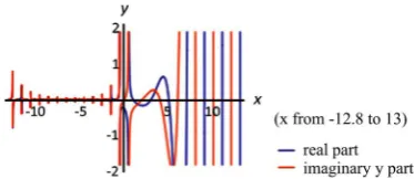
[image:12.595.207.540.164.322.2]

(47)

(13)

[image:13.595.278.465.71.152.2]

Figure A1. u

( )

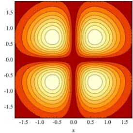
µ warped frequency domain.

Figure A2. u x

( )

time domain.

The 3d Navier Stokes system of equations for the incompressible viscid flow [9] is reducible to an extent that its general and exact solutions are determined by the (general and exact) solutions of the 2d Laplace equation in cylindrical coordinates (as above) as follows. We will call this solution a minimal solution.

Consider the NVS 3d systems of equations for the incompressible viscid flow:

(

)

2

t

ρ∂ +ρ ⋅∇ − ∇ = −∇ +µ ρ

∂

u _u _u _u _p _g₍₄₈₎

and µ_ρ=₌_{medium density}viscid constant

 (49)

Equation (48) per directional component in cylindrical coordinates:

2

2 2

2 2 2 2 2

1 1 2

r r r r

r z

r r r r

r

u u

u _u u u _u u

t r r r z

u

u u u u

g r

r r r r r r r z

θ θ

θ ρ

θ

ρ µ

θ θ

∂ ∂ ∂ ∂ 

+ + − +

 _∂ _∂ _∂ _∂ 

 

 ∂ ∂ ∂ ∂ 

∂ ∂  

= − + + _ _ _− + − + _

∂  ∂  ∂  ∂ ∂ ∂ 

P (50)

2 2

2 2 2 2 2

1 1 2

r

r z

r

u u u u u u u

u u

t r r r z

u u u u u

g r

r r r r r r z

θ θ θ θ θ θ

θ θ θ θ

θ ρ

θ

ρ µ

θ θ θ

∂ ∂ ∂ ∂

 ₊ ₊ ₊ ₊ 

 _∂ _∂ _∂ _∂ 

 

 ∂ ∂ ∂ ∂ 

∂ ∂  

= −_∂ + +  _∂ _ _∂ _− + _∂ + _∂ + _∂ 

 

P (51)

2 2

2 2 2

1 1

z z z z

r z

z z z

z

u

u _u u u _u u

t r r z

u u u

g r

z r r r r z

θ ρ

θ

ρ µ

θ

∂ ∂ ∂ ∂

 ₊ ₊ ₊ 

 _∂ _∂ _∂ _∂ 

 

 ∂ ∂ ∂ 

∂ ∂  

= − + + _ _ _+ + _

∂  ∂  ∂  ∂ ∂ 

[image:13.595.247.503.184.327.2]

(14)

DOI: 10.4236/am.2019.1011068 980 Applied Mathematics To solve the above 3d NVS system of equation we will have to reduce the r.h.s. of each equation to the sum of the pressure term and the external force and equating the Laplace expression in cylindrical coordinates to zero (solve up the Laplacian to get the velocity distribution), and then expand this using time con-volution to u

( )

x,t with the appropriate Gaussian diffusion Green’s function to solve the enclosed diffusion equation

2

t

ρ∂ = ∇µ

∂

u _u

(53)

and then use it to calculate the pressure distribution as follows

(

)

ρ

∇ =p g− u⋅∇ u (54)

To simplify this we will expand the super-position of discrete solutions Equa-tion (32) over the whole set of integers , then

( )

( ) (

)

( )

( ) ( )

( )

th

2

Green s function of diffusion eq. Taylor term of around

integrand of eq.(37) 1

2 ₄

0 0

e

convolution integral

1

, 2 e d

! 4

i ky k k

k f a

x y k k

k t

k

y a f a

u x t y t y

k t µ

δ θ

µ

π =∞ =−∞

− −

∞ =∞

=

∑

−

= π

π

∑

∫

’

(55)

( )

( ) ( )

( )

_{( )}

2 2

4 4

0

1 1

1 e e e

2 ! 2

x k k x

k t t a Df a

k

a f a

t t

t µ k t µ

ρ θ θ

µ µ

− −

=∞ −

=

−

π π

= =

∑

= ₍₅₆₎

The last function is rescaled along both axes compared to its time-domain version, and is called a “compressed” eigenfunction of the Mellin Transform op-erator, the corresponding transform pair on the time domain is equivalent with

( )

_{( )}

2

1 e e 4

t x a Df a _t

t

µ _θ

µ − π

π (57)

In two dimensions it will be congruent with

(

2 2

)

( 1) ( 2) 2

_{( )}

e e e

4

t x y _{a Df a} _{a Df a} t t

µ

θ µ

+ ₋ ₋

π ₍₅₈₎

The interested reader may try to derived it, the warped frequency 3d pressure distribution in Cartesian coordinates would be then, taking

0

g= (59) out of Equation (54) and disregarding the terms e−a Df a( )j _for _j₌_1,2,3_and the Heaviside time restriction in the different directions,

2 2 2 2

1 1 1 1

2 2 2 2

2 2

1 1 2 2

2 2

1 _Erf _exp _exp 1 _Erf _exp _exp ₍₆₀₎

2 4 4 2 2 4 2 2

1 _Erf _exp _exp

2 4 4 2

x y z

y x y z z x y z

k j

t t t t

t t

P

x y z x

P k

t t

P t

µ µ µ µ

µ µ

ρ

µ µ

µ

       

   

π π

−  − − −  − 

   

           

           

  _ _ _ _

π

 _{= −} _ _ _₋ _ ₋

     

     

 

2 2

1 1 2 2

2 2

2 2 2 2

1 1 1 1

2 2 2 2

1 _Erf _exp _exp ₍₆₁₎

2 4 4 2

1 _Erf _exp _exp 1 _Erf _exp _exp

2 4 4 2 2 4 2 4

z y z x

i

t _t t t t

x z x y y z x y

j i

t t t t

t t

µ _µ µ µ µ

µ µ µ µ

µ µ

  π      

 + _ _ −  − 

  _ _    

     

       

   

π π

−  − − −  −

   

          

            (62)

 

 

  



 

(15)

DOI: 10.4236/am.2019.1011068 981 Applied Mathematics using

(

)

(

)

2 2

, , exp exp ,

4 4

, , exp exp etc

4 4

k

i

x y

k u x y t

t t t

y z

i u y z t

t t t

µ µ µ

   

   

= − −

   

   

   

   

= − −

   

   

(63)

based on an i, j, k indexed classical Hamilton’ian unit vectors with magnitude

1

− _where _i2₌ _j2 ₌_k2₌_ijk_{= −}₁ _and

ij k= _, jk i= _, ki j= _, ij= −ji_, jk= −kj_,

ki

= −

ik

and where Erf(x) the Error function is, defined as

( )

2

0

2

Erf _z ₌ ze d−t _t

π

∫

(64) On the edge of the domain the following is true for the normal vectors

(

) ( )

0

k

u

u _{u x k u x}

n z

∂

∂ ₌ _≅ ₊ ₋ ₌

∂ ∂ etc. (65)

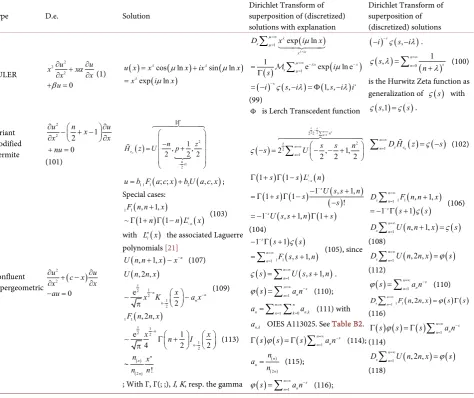
Please do see Figure A3. Figure A3 does show the contour graph of the warped frequency distribution in 3 dimensions.

The total energy of each wave system is equal on both the time and frequency domain [6] [7]. In symbols,

( )

2

( )

2 ₂

,

P t f t f f f x t t

∞ ∞ ∞

−∞ ∂ ∂ = −∞ ∂ = −∞ ∂ =

∫∫

∫



∫

 (66)

with above the expression for the Wigner-Ville Distribution function ( a class of dual energy distributions), and below, the integrand [is equivalent to the Ambi-guity Function] as defined in [3] [6] [7]

( )

_, _e2 2 2 e2 * e2 _d

2sinh 2sinh 2sinh

2 2 2

u u

r

iuft u fu fu

P t f f _u _u _u u

− +

− π

   

   

=    

   

   

∫

  (67)

( )

f

 is the analytical signal on the frequency domain and its Fourier Transform inverse x t

( )

on the time domain and _2_{the total (kinetic)}

ener-gy of the system and r is a warp parameter that may be set 1

2

− _{to yield a factor}

2 e e 1

u u

u

− (68)

in the integrand and what may be calculated with the Residue theorem. Expres-sion (65) will yield an unbounded wave energy-level of 2 ∞ _u

( )

_µ

2

_µ

−∞ ∂

=

_∫

 for

every component with

ζ

( )

1 = ∞_.

The Wigner-Ville time-frequency distribution function is a unitary affine function that suffices the following equation

( )

₂

( )

2

0

d , rd

f

t P t f t f f

f

ξ β

δ ξ β

∞ ∞

−∞

 

− − =

 

 

∫

  (69)

with

[ ]( )

( )

2 2

0 e d

i f i r

f f f f

ξ _β ₌ ∞ πξ π +β

∫

   (12).

(16)

[image:16.595.306.444.71.209.2]

Figure A3. Contour of 3d warped pressure distribution.

makes it also unbounded.

The last maximum value of the total energy is also supported by the fact that the Wigner-Ville Distribution function definition also does have a factor of the hyperbolic cosecant with half argument in its integrand (defined on

{

}

(

\ 2

)

C∞ _π _{, with poles at}

{

₂

{ }

}

k

i k _∈

π what may lead to variants of the improper Riemann contour integral [1]

( ) ( ) ( )

( )

1

( )

1

2sin d d

e 1 e 1

s s

x x

s s ς s i x i x

− −

∞ ∞

− −

π Γ = =

− −

∫

(70)

Below schematically, the application of the presented formulas for solving up the Laplace equation in cylindrical coordinates in an analytic signal analyzing model used by [6]. The constructed transformation is scale invariance:

An analytic signal analyzing model

( )f :



1 2

2 1

1 2

2

x i

x

i x α

ζ α =∞ π −

=

_{− π +} ₌

 

 

∑

,r_: x

Uξ →

( ) 2 ( )1 _{( )}

,r r1_e i a f _: f

Uξ f ₌a+ − πξ− af

 

2 1e

x i x

x

α =∞ − π =

∑

↓ (warping operator,

1 2

r= − , ξ =0,

ex

a₌ −

; 0,r 12

x x

Uξ = =− U

= )

↓

( ) ,r ( ) _:

f f Un f

ξ_ _₌ ξ _ _

   

   

(

)

2

1e 1

x i x x

x x x

α _δ _α

=∞ − π =∞

= = = −

∑



with  the Fourier Transform with ordinary unitary frequency

x

→ 

( )

[ ]

( )

(

)

( )

,

1 2 2

1 0

1 1

0

e d

d 1

r f x

x i x i

f x

x x U

a x x

x x x

ξ ξ

µ β β ξ

µ

β

µ

δ β

ζ µ

∞ =∞ − π −

− π

=

∞ =∞ −

=

 

 

= ⋅

= −

∑

∫

∑

∫

 

The result is equivalent with 1µ µi

(

µ α

_{( ) (}

)

_{ς µ α β},

)

α

− Γ +

− +

Γ for

0

ξ ≠ , µ= π + 2 iβ r, _a₌e−x_{and initial input}_{ς α}( )_{. Hence the}

factor _a− π2iβ_{may be moved to the integrand of the found Fourier}

Transform

( )

{

( )

}

2 1

1

e d

2

2 ,

f i f

f f f f

i

α ξ β µ

ξ µ α

µ ξ

µ α µ

µ α _{ξ β} α µ α

ς µ α β β α

∞ =∞ − − π + =

−∞

=∞ − −

− =

− − −

Γ +

= π +

Γ

Γ +

= π + −

Γ

∑

∫

(71),

(17)

DOI: 10.4236/am.2019.1011068 983 Applied Mathematics Out of the general solution is it clear that the distribution functions for u x

( )

and p x

( )

on the warped frequency domain do inherit the known singularities of the Dirichlet series, naturally depending on the begin-conditions which may cause shifts in singularities at

{ }

1 , removable singularities at

( )

log 2

log log

a p i

p p

π

− + ₍₇₂₎

with p a prime number as a consequence of the Euler denomination of the Di-richlet series (a

( )

+ ₌1_{for the Riemann Zeta function) in the form of the}

product formula

( )

_{( )}

1 prime

1 1

n s

s n a n n p _{a p p}

=∞ −

−

= = ₋

∑

∏

(73)

only for a n

( )

is totally multiplicative [17]. Solving up the zeros of the deno-minator in the last expression

( )

2

eπi₋_{a p p}−s₌0₍₇₄₎

does result in the mentioned complex removable singularities. So may be said that the distribution functions u x

( )

and p x

( )

are defined on C∞

(

\

{ }

)

for each component.

The begin-conditions may also dictate the periodicity of the general solution. There exists no general solution that is independent of the begin-solutions, since the solution is constructed out of the begin-conditions. The begin-conditions may cause singularities or may annihilate them, depending on the initial prob-lem and its basic solution. The basic solution of the Laplace equation in cylindrical coordinates, which is the solution core for both the velocity and pressure frequen-cy distributions (in the incompressible case) for the Navier Stokes equations in 2d and to certain extent also for the 3d version, does contain and consequently inhe-rits the singularities observed in the cited improper Riemann contour integral in particular or from the Dirichlet series in general. The input signal

( )

f ₁∞ fα

=

∑

 (75)

of the used model may manifest or cause singularities on both time and warped frequency domains with both the summation parameter indexed by f (hyperbo-las) and by α (polynomials). On the time domain the signal may experience singularities due to the vast powers that are used that may be unpractical for most commercial available micro-processors to compute [for example when f is chosen as the series of orthogonal polynomials like the Hermite polynomials or due to the known singularities of the Zeta function. On the warped frequency domain the singularities are due to the properties of the formed Dirichlet series output signals for both cases.

Interesting to note is that the so-called blow-up time within the numeric schemes may manifest whenever the numerical pivoting method strikes a known singularity of the general solution.

(18)

so-DOI: 10.4236/am.2019.1011068 984 Applied Mathematics lutions of the Laplace equation (read the momentum equation) are allowed, the motion solution of the 3d Navier Stokes equations for the viscid incompressible flow will become a (multi-dimensional) Gaussian function with no singularities on neither the time domain nor the warped frequency domain.

Appendix B

The Riemann Zeta Function represented as a Dirichlet Transform of discrete super-position of second order ODEs solutions.

The confluent hyper geometric functions are solutions to the Weber differen-tial equations, obtained after separation of variables when decomposing the Laplacian in cylindrical coordinates;

(

)

(

)

2

2 2 2

2

2 2 2

0

u _{c k x u} x

v _{c k x v} y

∂ _{− +} ₌

 ∂  _∂

 _{− −} ₌

∂ 

(76)

The substitution exp 2 4

x u w= ⋅ _− _

  converts the weber equation to

2

2 0

w _x w _w x

x υ

∂ ₋ ∂ ₊ ₌

∂

∂ (77)

with solution

( )

exp 2

4

x u H xυ

 

= ⋅ − 

 , where H xυ

( )

is the Hermite polynomial. In general the solutions of the second order ordinary confluent hypergeome-tric d.e.

(

)

2

2 0

w w

x c x aw

x x

∂ _{+ −} ∂ ₋ ₌

∂

∂ (78)

are of the form

(

)

(

)

1 2

1

1 ; ; , ,

w b F a c x b U a c x= + ₍₇₉₎

and are called the confluent hypergeometric function of the first and second kind respectively. The first kind version is also denoted as M a c x

(

, ,

)

or

(

a c x; ;

)

Φ _with

(

)

( )

1 1 ; ; 0 _!

n n n n

n

a z F a c x

c n

=∞ =

=

∑

₍₈₀₎

and a_{( )}n the Pochhammer symbol defined as

( )n

(

_{( )}

)

(

1

) (

1

)

a n

a a a a n

a Γ +

= = + + −

Γ (81).

An integral representation for U a b z

(

, ,

)

is

(

)

_{( )}

1

(

)

1

0

1

, , e z t a 1 b a d

U a b z t t t

a

∞ − ⋅ − − −

= +

Γ

∫

(82)

(19)

DOI: 10.4236/am.2019.1011068 985 Applied Mathematics The confluent hypergeometric function of the second kind, can be transposed to the improper contour integral

( )

1

d e 1

s

x x

i x

− −

−

∫

by choosing

b a

= +

1

_{, and} a s= _{. Namely}

(

)

_{( )}

1

0

1

, 1, en t s d

U s s n t t

s

∞ − ⋅ −

+ =

Γ

∫

(

, 1,

)

s

U s s₊ n ₌n− ₍₈₃₎

Taking an infinitely summation at both sides of the latter expression and substituting for n n*n and for s ₂s will

ς

( )

s _{emerge as super-position of the} solutions, namely

( )

2

1 _{2 2}, 1,

n n

s s

U n ς s

=∞ =

 ₊ ₌

 

 

∑

(84)

If we take 2

2

n _{instead of}_n2_{both sides as argument then the following}

ex-pression will arise

( )

2

1 _{2 2}, 1, ₂ 2

s n

n

s s n

U ς s

=∞ =

 

+ =

 

 

∑

(85)

( )

_{2 exp}2 2 1 _, 1_, 2

4 2 2 2

z z

D zυ υ U υ p

   

= −  − + 

    is a solution to the Weber d.e.

with p an integer and equal to null. D− −υ 1

( )

i z⋅ is the other linear independent

solution of Weber d.e.

( )

2

2 2

1 1 ₀

2 4

y _{z y z}

z υ

∂ ₊ _{+ −}  ₌

 

∂   (86)

With substitution

2

4

e x

y u= − _{converts the Weber d.e. to} u₂2 x u u 0

x

x υ

∂ ∂

+ − =

∂ ∂

with solution

( )

2

4 e x

y H zυ

−

= _.

( )

_{2 exp}2 2 _exp 2

( )

4 2 4 n

n

n z n z z e

D z = − _− _H _ _= _− _H z

 

    with

( )

₂ _, 1_, 2

2 2

n

n n

H z = U_− p+ z _

  (87)

the Hermite polynomial and H zen

( )

the modified Hermite polynomial. The modified Hermite polynomial is defined as

( )

₂2 ₂2 _, 1_, 2

2 2 2

2 n

n n

e n z n z

H z = − H _ _= U_− p+ _

    (88)

If we denote 1

2

p+ _by – 1 2

n₊ _{and compare it to the found expression of}

( )

s

(20)

( )

2 2

1

2 , 1,

2 2 2

s n n

s s n

s U

ς + =∞

=

 

= _ + _

 

∑

(89)

and substituting s by -s yields,

( )

1

2 2

1

2 , 1,

2 2 2

s n n n

s n n

s s n

s U

ς

=∞ =

− =∞

=

∑

 

− = _− − + _

 

∑

(90)

( )

2 2

1 2

1

2 , ,

2 2 2

n

n e

n z

H z U p

− +

 

 

−

 

= _ + _

 

 

(91)

If we interchange the parameters z and n with each other for H ze_n

( )

, and

su-perposition all the elements H ne_n

( )

with each other will the expression of

ς

( )

−s

emerge as above. The generalized Laguerre polynomials can be represented by

( ) ( )

_{( ) (}

1 , 1,

)

!

n a

n

u L x U n a x

n

−

= = +

− (92)

and are related to the Riemann Zeta function as described above. A known transform operator [12] that can transpose polynomial expressions into Dirich-let series is the DirichDirich-let transform

( )

_{( )}

1

( )

0

1 s _e z _d

s

D f x z f x z

s

∞ ₋ ₋

=

Γ

∫

(93)

that transforms the ordinary generating functions

( )

1 1

n n n n

f x =∞a x

=

∑

₍₉₄₎

(OGF) to 4

( )

1

n x n n

f x =∞a n− =

=

∑

(95) This transform is discussed in the chapter of combinatorics of [15] p. 177 and deals primarily with size conditions of x X≅ = ∈n of the permutations

( )

_k

( )

,

f x =

∑

f x k with auxiliary parameter variable k. The Dirichlet series with

( )

4 s 1 _x₁

f s =D f x ₌ (96)

where it may be used in conjunction with the Laplace-Borel Transform first, as intermediary aid, to first convert the Exponential Generating Functions (EGF)