C
2013. The American Astronomical Society. All rights reserved. Printed in the U.S.A.
TESTING HOMOGENEITY WITH GALAXY STAR FORMATION HISTORIES
Ben Hoyle1, Rita Tojeiro2, Raul Jimenez1,3,4, Alan Heavens5, Chris Clarkson6, and Roy Maartens2,7
1Institut de Ciences del Cosmos (ICC), Universitat de Barcelona (IEEC-UB), Marti i Franques 1, E-08024 Barcelona, Spain 2Institute of Cosmology & Gravitation, University of Portsmouth, Dennis Sciama Building, Portsmouth PO1 3FX, UK
3ICREA, Institucio Catalana de Recerca i Estudis Avancats, E-08010 Barcelona, Spain;http://www.icrea.es 4Theory Group, Physics Department, CERN, CH-1211 Geneva 23, Switzerland
5Imperial Centre for Inference and Cosmology, Astrophysics Group, Imperial College London,
Blackett Laboratory, Prince Consort Road, London SW7 2AZ, UK
6Astrophysics, Cosmology & Gravity Centre, and Department of Mathematics & Applied Mathematics,
University of Cape Town, Rondebosch 7701, South Africa
7Department of Physics, University of Western Cape, Cape Town 7535, South Africa Received 2012 September 27; accepted 2012 November 25; published 2012 December 12
ABSTRACT
Observationally confirming spatial homogeneity on sufficiently large cosmological scales is of importance to test one of the underpinning assumptions of cosmology, and is also imperative for correctly interpreting dark energy. A challenging aspect of this is that homogeneity must be probed inside our past light cone, while observations take place on the light cone. The star formation history (SFH) in the galaxy fossil record provides a novel way to do this. We calculate the SFH of stacked luminous red galaxy (LRG) spectra obtained from the Sloan Digital Sky Survey. We divide the LRG sample into 12 equal-area contiguous sky patches and 10 redshift slices (0.2 < z < 0.5), which correspond to 120 blocks of volume∼0.04 Gpc3. Using the SFH in a time period that samples the history of the universe between look-back times 11.5 and 13.4 Gyr as a proxy for homogeneity, we calculate the posterior distribution for the excess large-scale variance due to inhomogeneity, and find that the most likely solution is no extra variance at all. At 95% credibility, there is no evidence of deviations larger than 5.8%.
Key words: cosmology: theory – early universe – large-scale structure of universe Online-only material:color figures
1. INTRODUCTION
TheΛCDM concordance model is extremely successful, as it can fit most cosmological observations with just six free parameters (Komatsu et al.2011). Testing the assumptions that go into this model is vital, but it is often neglected. In particular, the model rests on the assumption of spatial homogeneity and isotropy on sufficiently large scales (for a review, see Clarkson & Maartens2010; Maartens2011; Clarkson2012). It is therefore appropriate and timely to devise observational tests that allow us to probe the homogeneity and isotropy assumptions. We know the isotropy assumption is well supported by detailed observations of the cosmic microwave background (CMB), which has shown that temperature variations are only one part in 105 across the sky. However, homogeneity is much
more difficult to probe. Homogeneity is not established by observations of the CMB and the galaxy distribution: we cannot directly observe homogeneity, since we observe down our past light cone, recording properties on two spheres of constant redshift and not on spatial surfaces that intersect that light cone. What these observations can directly probe is isotropy. In order to link isotropy to homogeneity, we have to assume the Copernican principle, i.e., that we are not at a special position in the universe. The Copernican principle is not observationally based; it is an expression of the intrinsic limitation of observing from one spacetime location.
The importance of testing the homogeneity assumption has been highlighted by the development of inhomogeneous “void” models which can potentially explain apparent acceleration without any exotic physics. By changing the mean density and expansion rate radially away from us, observations such as SNIa can be accommodated without any dark energy (see, e.g., Biswas
et al.2010; Marra & Notari2011; Clarkson2012for reviews.). However, it is difficult to fit all observations—in particular the combination ofH0and the CMB—without requiring significant
inhomogeneity or other departures from the standard model at early times as well (Nadathur & Sarkar2011; Bull et al.2012; Clarkson & Regis2011; de Putter et al.2012).
This implies that tests for homogeneity must be made throughout the history of the universe. Consistency tests which could uncover deviations from homogeneity can be used to probe consistency of observables on our past light cone (Clarkson et al.2008). Testing for the transition to homogene-ity in the galaxy distribution on the light cone, while assuming a Friedmann background, is another consistency test (Scrim-geour et al.2012). Probing inside our past light cone is harder, however, because we cannot observe it directly. One method is to use the Sunyaev–Zel’dovich (SZ) effect to observe CMB anisotropies from distant clusters (Goodman1995; Caldwell & Stebbins2008; Maartens2011). Another is to probe the thermal history in widely separated regions of the universe (Bonnor & Ellis1986), as it should, of course, be the same in the standard model.
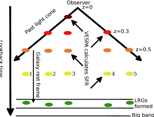
Figure 1.Illustration of the test of homogeneity. We assume that LRGs form at a similar cosmic time and have similar stellar formation rate histories (SFHs), which we illustrate by the galaxies’ changing color. VESPA recovers the SFH for each galaxy in the galaxies’ rest frame. We rebin the SFH to the common look-back time and compare the local star formation rate, for example, locations 1, 2,. . ., 5, to probe homogeneity. Galaxy worldlines are shown in comoving coordinates.
(A color version of this figure is available in the online journal.)
which encodes information about the histories of the component stellar populations, dust, and star formation. Various tools have been developed to extract this information (e.g., Heavens et al.
2000; Cid Fernandes et al.2005; Ocvirk et al.2006; Vincoletto et al.2012), of which we use the VErsatile SPectral Analysis8
(hereafter VESPA; see Tojeiro et al. 2007, 2009 for more details). These approaches rely on the assumption that the evolution of the stellar populations is well understood and that the current modeling of stellar population is accurate. We use VESPA to obtain the SFH within the time bin 11.5–13.4 Gyr of stacked luminous red galaxy (LRG) spectra located at different positions on the sky and at different redshifts. We compare the histories of different patches of the universe, using the local star formation rate as a proxy for homogeneity.
This Letter is organized as follows: in Section2 we briefly describe the applicability of the VESPA routine as a test of homogeneity, and then describe the data, star formation simulated data, and our method in Section 3. We present the results in Section4and conclude in Section5.
To calculate distances and to map from redshift to time, we assume a fiducial flat ΛCDM with best-fit WMAP7 (Komatsu et al. 2011) cosmological parameter values (ΩΛ,Ωm,Ωb, σ8, ns, H0 =0.729, 0.271, 0.045, 0.809, 0.966,
70.3 km s−1Mpc−1). Since we are looking for deviations from
homogeneity, it is conservative to assume this relation, which may be different in inhomogeneous universes (Heavens et al.
2011). Any viable dark energy or modified gravity model will have a background redshift–time relation that is close to the concordance model.
2. VESPA AND HOMOGENEITY
An illustrative diagram of our method is shown in Figure1. Here, for illustration only, we assume that LRGs form at a similar cosmic time and have similar SFHs, which we illustrate by the galaxies’ changing color. VESPA recovers the SFH for
8 http://www-wfau.roe.ac.uk/vespa/
Table 1
The Redshift Identifier and Range of the Redshift Slices, the Number of SDSS LRGs within Each Slice, and the Approximate Total Volume in Gpc3
Contained by the Redshift Slice
Redshift ID Range Ngals Total Volume
(Gpc3)
1 0.200< z <0.279 7874 0.90 2 0.280< z <0.308 9352 0.46 3 0.309< z <0.327 8532 0.34 4 0.328< z <0.342 8594 0.29 5 0.343< z <0.359 9181 0.36 6 0.360< z <0.376 8202 0.39 7 0.377< z <0.398 8754 0.55 8 0.399< z <0.424 8277 0.71 9 0.425< z <0.457 8272 1.00 10 0.458< z <0.537 8065 2.91
each galaxy along its own worldline (vertical lines in Figure1), allowing us to compare the SFH at different distances but at the same cosmic time, e.g., at positions 1, 2,. . . , 5. In practice, there is scatter in the SFH, due to sample variance on small scales and measurement error. We will consider these later, and seek additional variance from large-scale inhomogeneity.
3. DATA AND METHOD
Data. All of the galaxies used in this study were drawn from the Sloan Digital Sky Survey (see York et al.2000; Gunn et al.
2006; Smith et al.2002and references therein) Data Release 7 (SDSS DR7; Abazajian et al.2009). We use 8.5×10⁴galaxies
between the redshift range of 0.25 < z <0.55, selected to be LRGs (Eisenstein et al.2001) drawn from the VESPA database. We divide the SDSS survey footprint into 12 equal-area sky patches using HealPix9 (G´orski et al. 2005), and Nz =
10 redshift slices, whose widths are shown in Table1, together with the total number of galaxies, and the approximate volume of the SDSS survey in each redshift slice. We hereafter refer to the galaxies in each sky patch at each redshift slice as a “block” (B) of galaxies. We randomly select galaxies in each block into sub-samples of approximately 200 galaxies and stack the SDSS galaxy spectra for all galaxies in each sub-sample following the method presented in Tojeiro et al. (2011). Stacking the LRG spectra (as opposed to averaging the SFHs of individual galaxies in a block) allows us to recover the average SFH of a block with higher resolution in look-back time (see discussion in Sections 3.2 and 3.3 of Tojeiro et al.2011). We use VESPA to interpret the stacked spectrum in terms of a star formation and enforce VESPA to recover measurements in 16 time bins, τ. The time bins are in the rest frame of the stacked spectra, or alternatively the rest frame of the galaxy blockTB, and we refer
to these quantities as the star formation histories, SFH(TB, τ).
Additionally, we enforce VESPA to only allow star formation in bins whose starting times are after the start of the universe, calculated assuming our fiducial cosmology.
Methodology.We next add the age of the universe, calculated using our fiducial cosmology, at the average redshift of the galaxy blockTB, to the ages of the recovered VESPA bins for
the stacked spectra. We map the values of the SFH(TB, τ) to
a common frame SFH(0, τ) with bins denoted by τ, the look-back time with respect to the current epoch, and have chosen the lowest bin to be att =0. When we map the VESPA time binsτto the common time binτ, we choose to maintain the bin
[image:2.612.316.569.93.226.2]Figure 2.Start and end positions of the rest-frame (τ in the text) VESPA bins in look-back time, for each redshift slice. The continuous solid black lines show the locations of the common frame (τ) bins. We concentrate our test of homogeneity within the final bin between 11.5 and 13.4 Gyr.
(A color version of this figure is available in the online journal.)
widths to avoid overbinning the data. Figure2shows the start and end times of the rest-frameτ VESPA bins in look-back time (horizontal axis), for each redshift slice (vertical axis). The continuous solid black lines show the locations of the common frameτ bins with start times greater than 2 Gyr. LRGs form most of their stars vary early on, and so we concentrate our test of homogeneity within the greatest time binτ =15, which corresponds to a look-back time between 11.5 and 13.4 Gyr. The reason for this is that all stacks have considerably (almost two orders of magnitude) more star formation in this time bin than others, and have smaller fractional errors (see below for the error assignment). The distribution of a large number of random variables (recall each stack has ∼200 LRGs spectra) can be modeled as a Gaussian, following the central limit theorem. For lowerτ < 15 bins, some stacks have zero estimated star formation and larger fractional errors, skewing the distribution, which can no longer be modeled by a Gaussian, so we are unable to define a robust likelihood function.
The redshift slices of the blocks (recall that a block is a redshift slice/sky patch) are chosen to containNs 3 stacked spectra,
which are constructed from the (Ns) galaxy sub-samples within
the block. For each blockB, we calculate the averageAB, and
estimate the standard deviation of the block SFH,σB, from the
sub-samples. We determine the mean valueμofAB, and further
calculate the average value ofABfor all blocks at fixed redshiftz,
Az, and the standard deviation ofAzacross theNz=10 redshift
slices, which we denote asσz=σ(Az).
The dispersionσzis scatter arising from the rebinning of
solu-tions SFHB,i(TB, τ) of blocks at different redshifts to the
com-mon frame SFHB,i(0, τ). Note that block-to-block
[image:3.612.48.289.51.300.2]inhomogene-ity would contribute to this, but only at the level of one-twelfth of the variance, so it will affect our conclusions on the rms inho-mogeneity by only 4%. We will, however, make this correction.
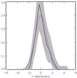
Figure 3.Studentt-distribution for the SDSS SFH data, assuming that the variance is due to a combination of small-scale (sub-block) sample variance, measurement error, and scatter due to rebinning from the galaxy rest frame to the present epoch. The vertical axis shows normalized frequency. The gray region gives the 95% spread of Gaussian random samples from the data and errors. We overplot the theoreticalts-distribution (dashed line).
(A color version of this figure is available in the online journal.)
We compute the Studentt-distributiontsfor all blocks:
ts =
AB−μ
σ2
B+σz2
, (1)
which determines the number of “combined error” σ ≡
√
σ2
B+σz2, or the departure the measurement AB, is from the
mean or notional value for the entire sample at each timeτ. For illustration, we compare the probability density function obtained by the above analysis, with the theoretical probability density function f(t) of the t-distribution with η = 10× 12 degrees of freedom, which has the analytic form given by
f(t)= √ 1 ηB(1/2, η/2)
1 + t
2
η
−(η+1)/2
, (2)
whereB(1/2, η/2) is the Beta function. We see in Figure3that the distribution oftsfollows the expected distribution reasonably
well. The gray shaded area shows the 95% range fortsstatistics
from 4000 Gaussian random samples of the SFH and errors. We now more formally model the data as having a Gaussian distribution but with the possibility of an extra frac-tional varianceVarising from inhomogeneity, i.e., we assume homogeneity and check for consistency using the likelihood of the data given by
PB(V)=
1
√
2π σV
exp−(AB−μ)2/2σV2
, (3)
σV2 =σB2+σz2+V μ2. (4)
If we assume a uniform prior forV, thenP(V)=ΠBPB(V) is
Figure 4.Ensemble probability that the dispersion seen in the values ofABis
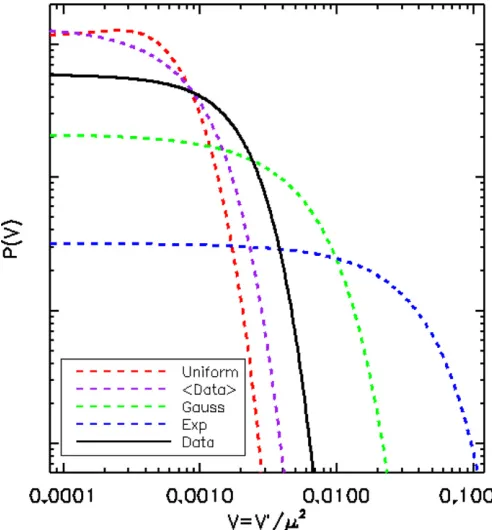
drawn from a Gaussian distribution aroundμ, as a function of an additional error componentV, which is scaled byμ2. The colored dashed lines show the probability for each simulated SFH and the black solid line shows the data. (A color version of this figure is available in the online journal.)
we showP(V) in Figure4for simulated data sets (sub-blocks) with variance NsσB2 for different SFHs: a continuous SFH, a
Gaussian SFH with mean 10 and standard deviation√2 Gyr, an exponential SFH with a scale length of 0.5 Gyr, and an SFH equal to the mean of the data. SFHs are rebinned to the common frame. We see in all cases that the posterior is correctly maximized at zero, and an upper limit dependent on the SFH.
4. RESULTS
In Figure 4, we show with the solid line the posterior distribution for the additional fractional varianceVin the SFH of the blocks. The most probable variance due to inhomogeneity is zero, and 95% of the posterior probability lies withinV < 0.0032. Hence the 95% credibility interval for the additional fractional inhomogeneity rms,√V (assuming a uniform prior on V), is 5.6%, or 5.8% if we include a correction for the rebinning. The colored lines show the different sets of simulated data. We see that only the uniform SFH has a peak that is not atV = 0; however, it is consistent with 0 at the<95% confidence level. We note that by artificially reducing the additional variance on each blockσB, the peak moves closer
toV =0.
5. CONCLUSIONS
Modern cosmology is built upon the assumption of homo-geneity which is inferred through the observation of isotropy (e.g., by the CMB radiation) and the Copernican principle, stat-ing that we do not occupy a preferred location.
Deviations from homogeneity, in particular, an inhomoge-neous background, e.g., Lemaitre-Tolman-Bordi (LTB) models in which massive void exist, can potentially explain the dimming
of distant supernovae without invoking dark energy. Testing ho-mogeneity is therefore an active area of research, and many tests have been devised, e.g., kinematic SZ effect.
In this Letter, we have performed a new observational test of homogeneity (Heavens et al. 2011) by examining the estimated SFHs in old stars from stacked spectra of SDSS LRGs (Eisenstein et al.2001) using VESPA. The data are blocks in 10 redshift intervals 0.025 < z < 0.55, with 12 equal-area angular bins.
We estimate the sample variance and measurement error aris-ing from small-scale (sub-block) variations by computaris-ing the error on the mean of the sub-blocks. Additionally, we include the scatter arising from rebinning to the present-day look-back time, and then perform a Bayesian analysis of any additional variance which may exist on large scales. Our test assumes ho-mogeneity and checks for consistency, and we find no evidence for extra variance, and a 95% upper limit to the credibility inter-val of a fractional variation of 5.8% in SFH between 11.5 and 13.4 Gyr. The typical block size is about 0.04 Gpc3.
The main uncertainty is in the stellar populations models employed by VESPA. However, this result can be easily ex-tended and improved upon with future spectroscopic surveys, e.g., BOSS (Dawson et al.2012), and as our knowledge of stel-lar population models increases. Although this is not a complete test of homogeneity, which would require investigation of the metric tensor itself, this limit on homogeneity is the first to come from within the past light cone, rather than being restricted to our past light cone. As such it is genuinely testing homogeneity rather than isotropy.
B.H. thanks Aday Robiana and Roland dePutter for use-ful discussions, the University of Cape Town for hospitality, and acknowledges grant No. FP7-PEOPLE- 2007- 4-3-IRG n 20218. C.C. and R.M. were supported by the South African NRF and by a UK Royal Society/NRF exchange grant. R.M. was supported by the SA SKA Project and the UK STFC (grant ST/H002774/1). Funding for the SDSS and SDSS-II has been provided by the Alfred P. Sloan Foundation, the Par-ticipating Institutions, the National Science Foundation, the US Department of Energy, the National Aeronautics and Space Ad-ministration, the Japanese Monbukagakusho, the Max Planck Society, and the Higher Education Funding Council for Eng-land. The SDSS Web Site ishttp://www.sdss.org/.
REFERENCES
Abazajian, K. N., Adelman-McCarthy, J. K., Ag¨ueros, M. A., et al. 2009,ApJS, 182, 543
Biswas, T., Notari, A., & Valkenburg, W. 2010,JCAP,11, 30 Bonnor, W. B., & Ellis, G. F. R. 1986, MNRAS,218, 605 Bull, P., Clifton, T., & Ferreira, P. G. 2012,PhRvD,85, 024002 Caldwell, R. R., & Stebbins, A. 2008,PhRvL,100, 191302
Cid Fernandes, R., Mateus, A., Sodr´e, L., Stasi´nska, G., & Gomes, J. M. 2005,MNRAS,358, 363
Clarkson, C. 2012,CRPhy,13, 682
Clarkson, C., Bassett, B., & Lu, T. H.-C. 2008,PhRvL,101, 011301 Clarkson, C., & Maartens, R. 2010,CQGra,27, 124008
Clarkson, C., & Regis, M. 2011,JCAP,2, 13
Dawson, K. S., Schlegel, D. J., Ahn, C. P., et al. 2012,AJ,145, 10 de Putter, R., Verde, L., & Jimenez, R. 2012, arXiv:1208.4534 Eisenstein, D. J., Annis, J., Gunn, J. E., et al. 2001,AJ,122, 2267 Goodman, J. 1995,PhRvD,52, 1821
Maartens, R. 2011,RSPTA,369, 5115
Marra, V., & Notari, A. 2011,CQGra,28, 164004 Nadathur, S., & Sarkar, S. 2011,PhRvD,83, 063506
Ocvirk, P., Pichon, C., Lan¸con, A., & Thi´ebaut, E. 2006,MNRAS,365, 46 Scrimgeour, M. I., Davis, T., Blake, C., et al. 2012,MNRAS,425, 116 Smith, J. A., Tucker, D. L., Kent, S., et al. 2002,AJ,123, 2121
Tojeiro, R., Heavens, A. F., Jimenez, R., & Panter, B. 2007,MNRAS,381, 1252
Tojeiro, R., Percival, W. J., Heavens, A. F., & Jimenez, R. 2011,MNRAS, 413, 434
Tojeiro, R., Wilkins, S., Heavens, A. F., Panter, B., & Jimenez, R. 2009,ApJS, 185, 1
Vincoletto, L., Matteucci, F., Calura, F., Silva, L., & Granato, G. 2012,MNRAS, 421, 3116