Applications of dynamical theory of X ray diffraction by perfect crystals to reciprocal space mapping

Received 14 May 2017 Accepted 7 July 2017

Edited by V. Holy´, Charles University, Prague, Czech Republic

Keywords:X-ray dynamical diffraction theory; reciprocal space maps; transversely restricted wavefronts; instrumental functions.

Supporting information:this article has supporting information at journals.iucr.org/j

Applications of dynamical theory of X-ray

diffraction by perfect crystals to reciprocal

space mapping

Vasily I. Punegov,a,b* Konstantin M. Pavlov,c,dAndrey V. Karpovaand Nikolai N. Faleeve

a_{Komi Research Center, Ural Division, Russian Academy of Sciences, Syktyvkar, 167982, Russian Federation,}b_Syktyvkar

State University, Syktyvkar, 167001, Russian Federation,c_{School of Science and Technology, University of New England,}

NSW 2351, Australia,d_{School of Physics and Astronomy, Monash University, VIC 3800, Australia, and}e_{Ira Fulton}

School, School of ECEE, Solar Power Laboratory, Arizona State University, 7700 South River Parkway, Tempe, AZ 85284, USA. *Correspondence e-mail: [email protected]

The classical dynamical theory of X-ray diffraction is expanded to the special case of transversely restricted wavefronts of the incident and reflected waves. This approach allows one to simulate the two-dimensional coherently scattered intensity distribution centred around a particular reciprocal lattice vector in the so-called triple-crystal diffraction scheme. The effect of the diffractometer’s instrumental function on X-ray diffraction data was studied.

1. Introduction

Recently, triple-crystal X-ray diffraction (Iida & Kohra, 1979; Zaumseil & Winter, 1982) has been successfully applied to investigate a variety of crystalline structures (Bhagavannar-ayana & Zaumseil, 1997; Kazimirov et al., 1990; Faleevet al., 2013; Lomov et al., 2014; Punegov, 2015) and X-ray optical elements (Jergelet al., 1999; Irzhaket al., 2015). Despite the fact that diffracted waves contain both coherent and diffuse scattered components, typically only the latter, caused by scattering on defects, is analysed, often only qualitatively. However, if one wants to quantitatively analyse the scattered intensity distribution (i.e.reciprocal space map) near a parti-cular reciprocal lattice vector where the coherent scattering is strong, some approximations of coherent scattering (Punegov, 2012) have to be used. These approximations are used because the current dynamical diffraction approach (Authier, 2001) assumes that the incident wave is a plane wave. Such an assumption results in the Dirac delta function intensity distribution (Kaganeret al., 1997) for the coherent scattering component, which makes impossible quantitative analysis of a diffraction pattern near the particular reciprocal lattice vector (Fig. 1).

It should be noted that quantitative analysis of coherently scattered waves was recently performed for crystals having a finite length in the lateral direction (Punegovet al., 2014, 2016; Pavlovet al., 2017). In this case the limited lateral size of such crystals restricts the illuminated area and, therefore, the diffracted intensity distribution is not a Dirac delta function anymore.

The diffraction of transversely restricted X-ray beams was considered (Berenson, 1989; Bushuev, 1998; Bushuev & Oreshko, 2007) in the case of the so-called double-crystal diffraction scheme. In particular, an approach using Green

ISSN 1600-5767

functions was employed by Bushuev (1998) and Bushuev & Oreshko (2007) to describe the spatially inhomogeneous Bragg diffraction by an ideal crystal. However, the results of Bushuev (1998) and Bushuev & Oreshko (2007) cannot be directly applied for the triple-crystal diffraction scheme because their approach integrates the angular distribution of the reflected wave, which can be resolved in the triple-crystal diffraction scheme because of the presence of the analyser crystal.

This paper aims to provide a quantitative analysis of two-dimensional diffraction intensity distributions of coherently scattered waves within the framework of dynamical diffraction theory in the case of transversely restricted wavefronts of the incident and diffracted waves.

2. Diffraction theory for transversely restricted X-ray waves

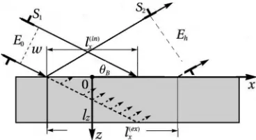
Let us consider dynamical X-ray diffraction by a perfect crystal in a Cartesian system of coordinates where thexandy axes are parallel to the top crystal surface, and thez axis is directed inside the crystal (Fig. 2). Thus, thexOzplane is the plane of diffraction. The angle between the wavevector of an incident monochromatic plane wave (of unit intensity) and the positive x direction is ¼Bþ!, where ! is the angular

deviation from the Bragg diffraction angle B (Fig. 2). The

entrance slit S1 determines the wave’s transverse width w.

Thus, the illuminated area of the top surface of the crystal is lðinÞ

x ’w=sinB. The transverse size of the reflected (scattered)

wave is limited by the exit slitS2, which defines a lateral size of

lðexÞ

x (Fig. 2) at the crystal surface. We also assume that the propagation distance between the particular slit and the crystal surface is small enough to satisfy the geometrical optics approximation.

For the sake of simplicity, we consider a symmetrical diffraction case in Bragg geometry (Fig. 2). The dynamical diffraction by an ideal crystal can be described by Takagi’s equations (Takagi, 1962) as follows:

cotB @ @xþ

@ @z

E0ð;x;zÞ ¼ia0E0ð;x;zÞ

þia_hEhð;x;zÞ; cotB

@ @x

@ @z

Ehð;x;zÞ ¼iða0þÞEhð;x;zÞ

þiahE0ð;x;zÞ; 8

> > > > > > < > > > > > > :

ð1Þ

where E0;hð;x;zÞ are the complex amplitudes of the trans-mitted and reflected electric field waves, respectively, ¼4cosB!= is the angular parameter used in the

double-crystal diffraction in the!–2mode, a0¼0=ð0Þ,

a_h;h¼C_h;h=ðh;0Þ,is the X-ray wavelength in a vacuum, 0;h¼sinB, C is the polarization factor, and g¼

r0 2_F

g=ðVcÞ are the Fourier components of polarizability,

with g¼0, h, h. Here Vc is the volume of the unit cell,

r0¼e

2_=ðmc2_{Þis the classical electron radius,eandmare the}

electric charge and mass of an electron,cis the speed of light, andFgis the structure factor. More information about Taka-gi’s equations and approximations used in them is given by Authier (2001) and Ha¨rtwig (2001).

Equation (1) can be simplified if both the incident plane wave and the crystal are homogeneous in thex direction, in which case there is no dependency on thexcoordinate:

@

@zE0ð;zÞ ¼ia0E0ð;zÞ þiahEhð;zÞ;

@

@zEhð;zÞ ¼iða0þÞEhð;zÞ þiahE0ð;zÞ; 8

> < > :

ð2Þ

which solution is well known in the case of Bragg geometry for an ideal crystal of thicknesslz(seee.g.Punegov, 1993; Punegov et al., 2010). Taking into account the boundary conditions at the top [E0ð;z¼0Þ ¼1] and the bottom [Ehð;z¼lzÞ ¼0] surfaces of the crystal, the amplitude transmission coefficient TðÞ ¼E0ð;z¼lzÞ and the amplitude reflection coefficient RðÞ ¼Ehð;z¼0Þare as follows:

TðÞ ¼exp½iða0þ1Þlzð=QÞ; ð3Þ

RðÞ ¼ah ½expðilzÞ 1=Q; ð4Þ

where ¼ ð 2_4a

hahÞ

1=2

, 1;2¼ ð Þ=2, Q¼ 1expðilzÞ 2and ¼þ2a0.

However, if the incident wave is transversely restricted, then one cannot use equation (2) and has to employ the more

Figure 2

A diffraction scheme for the case of dynamical diffraction by a crystal of thicknesslzwhen the incident and the diffracted waves are transversely limited by slitsS1andS2, respectively.

Figure 1

general equation (1), because the wave amplitudes will be functions of thexcoordinate.

We will use the following definitions of the inverse and direct Fourier transforms:

E0;hð;x;zÞ ¼ 1 2

Zþ1

1

dexpðixÞEE^0;hð; ;zÞ; ð5Þ

^ E

E0;hð; ;zÞ ¼ Z þ1

1

dxexpðixÞE0;hð;x;zÞ; ð6Þ

whereis the coordinate in Fourier space which corresponds to thexcoordinate in real space. If we substitute equations (5) and (6) into equation (1), we obtain

@EE^0ð; ;zÞ

@z ¼iða0cotBÞ ^ E

E0ð; ;zÞ þiahEhE^ ð; ;zÞ;

@

^ E

Ehð; ;zÞ

@z ¼iða0þcotBÞ ^ E

Ehð; ;zÞ þiahEE^0ð; ;zÞ:

8 > > > > < > > > > :

ð7Þ

Fourier transforms of the wave amplitudes in equation (7) allows us to transform the two-dimensional system of equa-tions (1) to the one-dimensional system of equaequa-tions (7) in real space, which has analytical solutions. Note that the structure of equation (7) is similar to that of equation (2), exclusive of different coefficients.

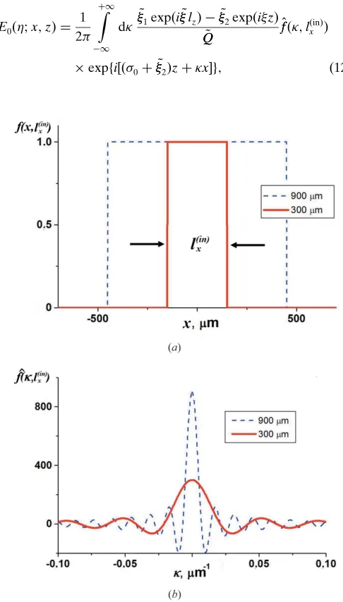
To solve equations (7) we need to define their boundary conditions. Let us assume that the amplitude of the restricted incident wave at the top crystal surface is defined by

fðx;lðinÞ

x Þ ¼

1 lðinÞ

x =2xl

ðinÞ x =2; 0 otherwise:

ð8Þ

This function is shown in Fig. 3(a), where lðinÞ

x is 300 and 900mm. The function fðx;lðinÞ

x Þ can be also represented as a Fourier integral:

fðx;lxðinÞÞ ¼ 1 2

Z1

1

^

ffð;lðxinÞÞexpðixÞd: ð9Þ

In Fourier space this function has the following analytical expression:

^ ff ;lðxinÞ

¼sinðl

ðinÞ x =2Þ

=2 : ð10Þ

The functionff^ð;lðinÞ

x Þfor 300 and 900mm widths of the inci-dent beam on the crystal surface is shown in Fig. 3(b).

If the amplitude of the incident wave at the crystal surface is described by equation (8), this corresponds to the following boundary condition in real space: E0ð;x;0Þ ¼fðx;l

ðinÞ x Þ. Using equations (6) and (10), we can also define the boundary condition for the mixed representationEE^0ð; ;0Þ ¼ff^ð;l

ðinÞ

x Þ

at the top crystal surface (z= 0). The boundary condition for the diffracted wave (in the mixed representation) at the bottom surface of the crystal (z=lz) isEE^hð; ;lzÞ ¼0.

Using these boundary conditions, we can write down analytical solutions to the system of equations (7) in the mixed (in real and Fourier space coordinates) form for 0 <z<lz:

^ E

E0ð; ;zÞ ¼

~

1expði~lzÞ ~2expði~zÞ

~ Q Q

^ ffð;lxðinÞÞ

exp½ið₀þ~₂Þz;

^ E

Ehð; ;zÞ ¼ah

expði~lzÞ expði~zÞ ~

Q Q

^ ffð;lðinÞ

x Þ

exp½ið₀þ~₂Þz;

ð11Þ

where 0¼ ða0cotBÞ, QQ~ ¼~1expði~lzÞ ~2, ~1;2¼

ð~~Þ=2,~¼ ð~24ahahÞ

1=2

and ~¼þ2a02cotB.

This mixed form solution (11) can be used to obtain [after substitution into equation (5)] the amplitudes of the reflected and transmitted waves as functions of thexandzcoordinates and the angular parameter:

E0ð;x;zÞ ¼

1 2

Z þ1

1

d~1expði~lzÞ ~2expðizÞ

~ Q Q

^ ffð;lðxinÞÞ

expfi½ð0þ~2Þzþxg; ð12Þ

Figure 3

Ehð;x;zÞ ¼ ah 2

Z þ1

1

dexpði

~

lzÞ expði~zÞ

~ Q Q

^ ffð;lðxinÞÞ

expfi½ð0þ~2Þzþxg: ð13Þ

These integral solutions (12) and (13) to Takagi’s equations (1) were obtained for particular boundary conditions (8) and (10). At the bottom of the crystal (z = lz) the amplitude of the transmitted wave can be obtained from equation (12) as a function of thexcoordinate and the angular parameter:

Tð;xÞ ¼ 1

2 Zþ1

1 d

~

~ Q Q ^

ffð;lðxinÞÞexpfi½ð0þ~1Þlzþxg:

ð14Þ

By substitutingz= 0 in equation (13) we obtain the amplitude of the reflected wave at the top surface of the crystal:

Rð;xÞ ¼ah

2 Z þ1

1

dexpði

~

lzÞ 1 ~ Q Q

^

ffð;lðxinÞÞexpðixÞ: ð15Þ

The wider the incident X-ray wave, the narrower the function ^

ffð;lðinÞ

x Þis in Fourier space (Fig. 3). In the case of the incident plane wave the function ff^ð;lðinÞ

x Þ transforms into the Dirac delta function [see equations 21.9-18c and 21.9-11 of Korn & Korn (1968) and also Weiet al.(2002)]:

lim lxðinÞ!1

^ ff ;lðxinÞ

¼ lim lðinÞx !1

sinðlðinÞ x =2Þ

=2 ¼2 ðÞ: ð16Þ

Then, in the case of the plane incident wave [see equation (16)], solutions (14) and (15) transform into the well known amplitude transmission [equation (3)] and reflection [equation (4)] coefficients, respectively.

3. Reflection and transmission X-ray intensity distribution maps inside a crystal

Let us consider an incident plane monochromatic X-ray wave havingpolarization and unit intensity. This wave illuminates a crystal, and the angle between the wavevector of the incident wave and the X axis is 0¼Bþ!0. Then the transmitted

ITð0;x;zÞ and reflected IRð0;x;zÞ intensities inside the

crystal are defined as follows:

ITð0;x;zÞ ¼ jE0ð0;x;zÞj 2

;

IRð0;x;zÞ ¼ jEhð0;x;zÞj 2

; ð17Þ

where the amplitudesE0;hð0;x;zÞare given in equations (12)

and (13),0¼4cosB!0=, and!¼!0is a small deviation

from the exact Bragg angle.

The numerical modelling is performed for a transversely restricted X-ray wave having the wavelength¼0:154056 nm (CuK1radiation) in the case of an Si(111) reflection. The

angular position was corrected on the refraction shift proportional to the real component ofa0in equation (1). The

Fourier components of polarizability, g, where, g¼0;h;h, were obtained from Sergey Stepanov’s X-Ray Server

(Stepanov & Forrest, 2008). The primary Bragg extinction length (Authier, 2001) for the Si(111) reflection is lðextzÞ ¼jsinBj=ðCjhjÞ= 1.51mm. The Bragg angle for this reflection is 14.221 _{and the interplanar distance} d111¼3:1355 A˚ . The thickness of the crystal islz= 100mm.

Fig. 4 shows the reflection and transmission X-ray intensity distribution maps at different 0 inside a crystal for l

ðinÞ

x =

300mm. These maps were calculated using equations (12), (13) and (17). The contours of equal intensity are shown on a logarithmic scale with a step size of 0.58 for intensity. Note that, although the thickness of the silicon crystal is 100mm, Fig. 4 shows only the upper part of the crystal, for the z coordinate varying from 0 to 5mm. At the larger depth both the transmitted and reflected intensities become negligible (in the vicinity of the Bragg diffraction angle) owing to primary extinction effects (Authier, 2001).

If the angle of incidence is exactly the Bragg angle (i.e. ₀¼!₀¼0, ₀¼_B), then the intensity of the transmitted and reflected waves exponentially decreases with the crystal depth: IT;Rð0;x;zÞ /expð2z=l

ðzÞ

extÞ (Authier, 2001) due to

primary extinction. Some intensity oscillations are observed on the left side of the transmission and reflection intensity distribution maps in Figs. 4(a) and 4(b). There the area of the maximum transmitted intensity corresponds to the area of the minimum reflected intensity. These oscillations can be described as pseudo-Pendello¨sungoscillations, well known for the Laue diffraction case (Authier, 2001). Evidently, the transverse limitation of the incident beam shapes the area of the crystal where the diffraction occurs.

Figure 4

The transmission (a), (c) and reflection (b), (d) X-ray intensity distribution maps (on a logarithmic scale with a step size of 0.58 for intensity, where red and blue correspond to the highest and lowest intensity, respectively) at!0= 0 (a), (b) and!0= 0.30 0 (c), (d) inside a

crystal for the case of the illuminated arealðinÞ

To the left of the line AC (Fig. 5) the lattice planes do not participate in the X-ray diffraction. Therefore, the scattering crystal volume is limited by the top surface ABY and bottom surface CDY planes as well as by the ACY plane. Conse-quently, along the line AC, for example, at the point L (see Fig. 5, where T is the transmitted wave and R is the reflected wave), the X-ray wave is incident to the scattering atomic planes in Laue geometry.

Note that the intensity of the transmitted wave decreases with depth (i.e.in the positivezdirection) owing to primary extinction. The period of the pseudo-Pendello¨sungoscillations (in the x direction) is lðextxÞ ¼jcosBj=ðCjhjÞ ¼l

ðzÞ extcotB.

Bushuev (1998) introduced a longitudinal extinction length _x¼lextðzÞcotB, which differs only by a coefficientfrom the

period of the pseudo-Pendello¨sungoscillations shown above. Moving to the right from the line AC in the positive x

direction, X-ray diffraction predominantly transfers into the Bragg diffraction case, and, hence, the amplitude of the pseudo-Pendello¨sung oscillations reduces (Fig. 4). This physical phenomenon resembles the Bragg–Laue diffraction case in lateral (having a finite length in the lateral direction) crystals (Punegovet al., 2016).

For the angular deviation !0 = 0.300 (Figs. 4c and 4d) the

extinction length increases, while the intensity of the trans-mitted and reflected waves now decreases with the depth more slowly:IT;Rð0;x;zÞ /exp½2zð1

2 0=4ahahÞ

1=2 =lðextzÞ.

Whereas the left boundary (AC) of the transmitted and reflected waves is well defined, the right boundary (near the BD line) is more blurred owing to the dynamic interaction of X-ray waves inside the crystal (Fig. 4). This effect becomes more evident with the increase of the angular deviation from the exact Bragg condition (Figs. 4cand 4d), which is consistent with the conclusions of Berenson (1989).

Thus, a transversely limited incident X-ray wave ‘cuts’ in a plane parallel crystal slab a laterally limited volume with a cross section shaped as a parallelogram, the right-hand side of which is diffused.

4. The triple-crystal diffraction scheme

The triple-crystal X-ray diffraction scheme allows one to register two-dimensional maps of the diffracted intensity distribution in reciprocal space. These two-dimensional maps are dependent on two angular parameters, ! and ", which specify the angular positions of the investigated sample and the analyser crystal (Iida & Kohra, 1979), respectively. In the symmetrical Bragg geometry these two angular parameters are related to the projections qx;y of the deviation of the diffraction vector from the reciprocal lattice point:

qx¼ksinBð2!"Þ;

qz¼ kcosB";

ð18Þ

where k¼2=. In the case of the triple-crystal diffraction scheme [the detailed geometry of this scheme is shown by Nesterets & Punegov (2000)] the angular variable can be written as

¼qxcotBqz: ð19Þ

To proceed from the double-crystal to the triple-crystal diffraction scheme in the case of spatially restricted waves, the amplitudes E0;hð;x;zÞ in equations (12) and (13) must be Fourier transformed with respect to theqxvariable. Then, the intensity of the reflected X-ray wave at the top surface of the crystal is written as

IRðqx;qzÞ ¼

1 lnorm

Z lðexÞx =2

lðexÞx =2

dxexpðiqxxÞEhð;x;0Þ

2

: ð20Þ

In equation (20) we took into account that the X-ray wave reflected by the sample is incident on the analyser crystal (or a two-dimensional detector) as a transversely restricted wave with a lateral width oflðexÞ

x . After some algebra, equation (20) can be represented in the following (cross-correlation) form:

IRðqx;qzÞ ¼

ah 2lnorm

Z þ1

1

expði~lzÞ 1 ~ Q Q

^

ffð;lðxinÞÞff^ðqx;l ðexÞ x Þd

2

: ð21Þ

Here lnorm is equal to the smaller of l ðinÞ

x and l

ðexÞ x ; ~

¼ ð~24ahahÞ

1=2

, ~¼2a0qzþ ðqx2ÞcotB and

^

ffðqx;l ðexÞ

x Þ ¼sin½ðqxÞl ðexÞ

x =2=½ðqxÞ=2. Now we consider some special cases.

4.1. Unrestricted reflected X-ray wave (absence of slitS2)

Consider the case where slitS2is absent, and the analyser

crystal and detector collect the entire reflected wave. Mathe-matically, this means that lðexÞ

x ! 1. Then, the function ^

ffðqx;l ðexÞ

x Þ ¼2 ðqxÞ, which can be substituted into equation (21) to obtain the solution for the reflected wave intensity distribution in reciprocal space:

Figure 5

IRðqx;qzÞ ¼ ah

expðilzÞ 1 Q sincðqxl

ðinÞ x =2Þ

2

; ð22Þ

where ¼ ð 24ahahÞ

1=2

, _1;2¼ ð Þ=2, Q¼

₁expðilzÞ 2, ¼2a0qxcotBqz and sincðxÞ ¼ sinðxÞ=x.

Note that in the expression for the termqxcotBis taken

with a minus sign. The intensity in equation (22) depends on the lateral sizelðinÞ

x of the incident X ray wave. In the case of an !–2 scan (an analogy of the double-crystal diffraction scheme) the result shown in equation (22) coincides with the conclusions of Bushuev (1998) and Bushuev & Oreshko (2007) obtained for the double-crystal diffraction scheme.

Fig. 6 demonstrates how the reciprocal space maps (RSMs) near the Si(111) reciprocal lattice vector depend (in the absence of slit S2) on the lateral width, lxðinÞ, of the incident X-ray wave, defined by slit S1. In the case of a wide

(lðinÞ

x ¼900mm) incident beam, an inclined oscillating streak, related to the width of the incident beam, and a narrow vertical streak of the so-called main peak (see Fig. 6a) appear on the RSM. The angle between the main streak and the oscillating streak is equal to the Bragg angle. In the triple-crystal diffraction scheme this oscillating streak is usually called the analyser pseudo-peak. The length and width of this inclined oscillating streak increase while the lateral width of the incident wave decreases (Fig. 6band 6c).

4.2. Unrestricted incident plane wave (absence of slitS1)

Consider the case when a laterally unrestricted plane X-ray wave is incident on the top surface of the crystal. This means that lðinÞ

x ! 1 and, as shown above [see equation (16)], ^

ffð;lðinÞ

x Þ ¼2 ðÞ, which can be substituted into equation (21):

IRðqx;qzÞ ¼ ah

expðilzÞ 1 Q sincðqxl

ðexÞ x =2Þ

2

; ð23Þ

where ¼ ð 24ahahÞ

1=2

, 1;2¼ ð Þ=2, Q¼ 1expðilzÞ 2and ¼2a0þqxcotBqz.

Equation (23) demonstrates that the intensity of the reflected (scattered) wave depends on the lateral widthlðexÞ

x . In addition, the termqxcotB, present in equation (23) through

the angular parameter , has a positive sign in contrast to equation (22). Also note that expressions (22) and (23) have a very similar form. The difference is only in parameters lðinÞ

x $l

ðexÞ

x in the sinc function andqxcotB$qxcotBin .

Fig. 7 demonstrates the calculated RSMs for the laterally unrestricted incident X-ray wave while the lateral size of the reflected wave is either 900 or 300 or 30mm. Comparison of Figs. 6 and 7 shows that the RSMs for the same size of the incident and reflected beams have a mirror symmetry with respect to the vertical axis. This directly follows from

Figure 6

Calculated RSMs (on a logarithmic scale with a step size of 0.18 for intensity, where red and blue correspond to the highest and lowest intensity, respectively) near the Si(111) reciprocal space vector for different lateral widths,lðinÞ

x , of the incident wave: (a) 900mm, (b) 300mm, (c) 30mm. The lateral width of the reflected wave is unrestricted.

Figure 7

Calculated RSMs (on a logarithmic scale with a step size of 0.18 for intensity, where red and blue correspond to the highest and lowest intensity, respectively) near the Si(111) reciprocal space vector for different lateral widths,lðexÞ

equations (22) and (23), where the terms qxcotB in the

expressions for the angular parameter have opposite signs. If in equation (23) the lateral width of the reflected wave lðexÞ

x ! 1, then ff^ðqx;lxðexÞÞ ¼2 ðqxÞ and the reflected wave intensity (in the case of unrestricted incident and reflected X-ray waves) is

IRðqx;qzÞ ¼ 2 ðqxÞah

expðilzÞ 1 Q

2

: ð24Þ

4.3. Formation of RSMs in the general case of the transversely restricted incident and reflected X-ray waves

In the general case when both the incident and reflected waves are transversely restricted (by slitsS1andS2), the RSMs

can be calculated using equation (21), which provides a general solution for transversely restricted waves. Fig. 8 shows simulations of RSMs near the Si(111) reciprocal space vector for a crystal having a thicknesslz= 100mm for three different lateral sizes of the incident wave, lðinÞ

x , namely 900, 300 and 30mm, while the lateral size of the reflected wave, lðexÞ

x =

300mm, is still unchanged.

If both waves (transmitted and reflected) are spatially restricted, a mirror symmetry of inclined streaks (with respect to the vertical axis) is observed in the RSMs. The length of these streaks depends on the size of slits S1 and S2: the

narrower the slit, the wider and longer the intensity streak in the RSM. The direction of the streaks in reciprocal space coincides with the direction of the monochromator and analyser pseudo-peaks in the triple-crystal diffraction scheme. If the lateral dimensions of the incident and diffracted beams are equal, the RSM has a symmetrical shape (Fig. 8b). If one of the slits, for instance, S1, is significantly narrower than the

other slit, S2, changes in the shape and size of the intensity

streaks are evident (Fig. 8c).

4.4. Cross-sectional analysis of RSMs

First we consider the situation when slitS2is absent. Then

the RSMs’ cross sections can be calculated using equation (22), which may be represented as a product of two functions:

IRðqx;qzÞ ¼ jR1ðqx;qzÞR2ðqxÞj

2

, where R1ðqx;qzÞ ¼ah

½expðilzÞ 1=Q and R2ðqxÞ ¼sinðqxl ðinÞ x =2Þ=ðqxl

ðinÞ

x =2Þ. The first function,R1ðqx;qzÞ, coincides (in its form) with the

clas-sical solution (4) and depends on the thickness of the crystallz. The second function,R2ðqxÞ, which squared equals the Laue

Figure 8

Calculated RSMs (on a logarithmic scale with a step size of 0.18 for intensity, where red and blue correspond to the highest and lowest intensity, respectively) near the Si(111) reciprocal space vector for different lateral widths of the incident beam: (a) 900mm, (b) 300mm, (c) 30mm. The lateral size of the reflected beam is 300mm.

Figure 9

interference function, is determined by the width of the top crystal surface illuminated by the incident X-ray wave.

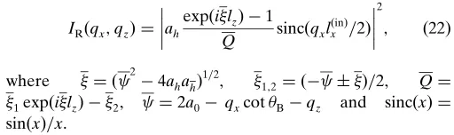
Fig. 9 shows cross sections (along theqxandqzaxes) of the simulated RSMs near a (111) reciprocal space vector of a perfect Si(111) crystal for three different lateral widths of the incident beam. The!–2diffraction curves or, in other words, the qz cross section of the RSMs at qx = 0 for all three presented RSMs are identical and represent the Darwin curve (Fig. 9a). Thus, for a thick perfect crystal the lateral width of the incident beam does not affect the profile of theqzcross section of the RSM. The rocking curves (!curves) or, in other words, theqxcross sections of Si(111) RSMs atqz= 0 show dependency on the lateral width of the incident beam (see Fig. 9b): the smaller the lateral width of the incident beam, the wider the rocking curve.

Often the cross sections of experimental RSMs are presented as functions of the angular deviation,!, from the exact Bragg position. In the!–2scanning mode or in theqz cross-sectional scan, when for all angular positions !¼"=2 (i.e. qx = 0), one obtains that ¼2a0þ2kcosB!. Taking

into account thatR2ðqx¼0Þ ¼1, the resulting expression for the reflected intensity isIRðqx¼0; !Þ ¼ jah½expðilzÞ 1=Qj

2

, where ¼ ½ð2a0þ2kcosB!Þ

2

4ahah

1=2

. This expression shows that the cross section in the!–2scanning mode does not depend on the lateral width of the incident X-ray beam.

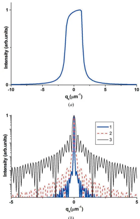
Fig. 10(a) shows a Darwin curve in the vicinity of the 111 reflection for a 100mm thick Si(111) perfect crystal as a function of the angular deviation !. The full width at half-maximum (FWHM) of the diffraction curve is about 700_.

In the !-scan mode (qz= 0, qx¼2ksinB!, ¼2a0

2kcosB!), the reflected intensity can be written as

IRð!;qz¼0Þ ¼ jR1ð!;qz¼0Þj

2

½R2ð!Þ 2

. Unlike the !–2 scan, the reflected intensity depends on the product of two functions. The first,jR1ð!;qz¼0Þj

2

¼ jah½expðilzÞ 1=Qj

2

, represents the!–2diffraction curve, while the second one,

½R2ð!Þ 2

¼ f½sinðksin_B!lðinÞ

x Þ=ðksinB!l ðinÞ x Þg

2

, depends on the lateral width of the incident X-ray wave and is a narrow function of the angle ! (see Fig. 10b, curve 2), where ¼ ½ð2a02kcosB!Þ

2

4ahah

1=2

. Note thatjR1ð!;qz¼0Þj 2

¼ jR1ðqx¼0;!Þj

2

, that is the!scans of the Darwin curves for the vertical [jR1ðqx¼0;!Þj

2

] and lateral [jR1ð!;qz¼0Þj 2

] cross sections of the RSMs are mirrored.

Fig. 10(b) shows an!scan (blue curve 1) for a 100mm thick Si crystal in the vicinity of the 111 reflection, where the lateral width of the incident X-ray beam lðinÞ

x ¼300mm. This ! rocking curve (blue curve, 1) is a product of the narrow Laue interference function (red curve, 2) and a broad Darwin curve (black curve, 3). Thus the narrow curve ½R2ð!Þ

2

determines the narrow shape of the ! scan, having an FWHM of less than 100_.

5. Instrumental function

To analyse real experimental data, the analytical results obtained in previous sections should be complemented by an instrumental function, which contains information about the monochromator and analyser crystals used in the experiment. There are numerous theoretical and experimental analyses of instrumental functions for different types of diffractometers (Zaumseil & Winter, 1982; Holy´ & Mikulı´k, 1996; Fewster, 1989; Gartsteinet al., 2001; Boulleet al., 2002; Mikhalychevet al., 2015). The first theoretical description of how different configurations of collimator/monochromator and analyser crystals in the triple-crystal diffractometer affect the regis-tered intensity was published by Zaumseil & Winter (1982). Recent modelling of instrumental functions based on semi-analytical backward ray tracing for high-resolution X-ray diffractometers was reported by Mikhalychevet al.(2015). If the main X-ray optical elements (e.g. collimators/mono-chromators and analyser crystals) employ multiple reflections (Mikhalychevet al., 2015), the intensity of the monochromator and analyser pseudo-peaks is significantly reduced and is sometimes totally suppressed (Fewster, 1989). Therefore, an investigation of the effects of the instrumental function on RSM distortions is essential for the correct interpretation of experimental RSMs.

Figure 10

(a) The !–2diffraction curve IRðqx¼0; !Þ ¼ jR1ðqx¼0; !Þj

2

in the vicinity of the 111 reflection for a 100mm thick Si(111) crystal as a function of the angular parameter!. (b) The blue curve 1 is the rocking curve IRð!;0Þ ¼ jR1ð!Þj

2_½R 2ð!Þ

2

for an incident X-ray beam with the lateral widthlðinÞ

x ¼300mm; the red curve 2 is the function½R2ð!Þ 2

In our analysis we suppose that the scattered intensity is already integrated along theqydirection. In addition, we will also neglect non-monochromaticity of the incident radiation, because its impact is much smaller than that caused by the resolution functions of the monochromator and analyser crystals (Mikhalychev et al., 2015). Let us now consider the angular distribution of the scattered intensityIðRinsÞðqx;qzÞthat

is recorded in the triple-crystal diffraction scheme with slitsS1

andS2, which spatially restrict the incident and the reflected

waves, respectively.

In the case of symmetrical diffraction the angular deviation of the sample, !, and the analyser crystal,", are connected with projectionsqx;z(Nesterets & Punegov, 2000):

!¼qxcosBqzsinB

hcosB

; "¼ qz

kcosB

; ð25Þ

where his the vector of the reciprocal lattice. In the experi-ment the angular deviation of the investigated sample, !, is related to the angular deviation of the monochromator crystal by =!and to the angular deviation of the analyser crystal by = !". The appropriate reflection coefficients of the

monochromator and analyser crystals are then RM_{ð!Þ and}

RA_{ð!"Þ, respectively.}

Thus, the normalized diffracted intensity distribution in reciprocal space, corrected by the instrumental function, can be represented in the following form:

IRðinsÞðqx;qzÞ ¼ R

þ1

1 R þ1

1 dq0

xdq 0 zR

M

ðq0 x;q

0 zÞR

A

ðq0 x;q

0

zÞIRðqxq 0 x;qzq

0 zÞ R

þ1

1 R þ1

1 dq0

xdq 0 zR

M_ðq0 x;q

0 zÞR

A_ðq0 x;q

0 zÞ

;ð26Þ

where

RMðq0x;q 0 zÞ ¼R

M

q

0

xcosBq 0 zsinB

hcos_B

;

RAðq0x;q 0 zÞ ¼R

A q 0

xcosBq 0 zsinB

hcosB

þ qz

kcosB

ð27Þ

are the reflection coefficients for the monochromator and analyser crystals, respectively; IRðqx;qzÞ is the scattering intensity, calculated using equation (22).

We can use for the functionsRM;A_{ð!Þ ¼ jrð!Þj}2

the reflec-tion coefficients for semi-infinite perfect crystals, where the amplitude reflection coefficient,rð!Þ, is the well known func-tion (Authier, 2001)

rð!Þ ¼ a

M;A

h =

M;A

1 ð!Þ if Im½

M;A_ð!Þ<0;

aMh;A=

M;A

2 ð!Þ if Im½ M;A

ð!Þ>0:

ð28Þ

The coefficients M;A_{ð!Þ and} M;A

1;2 ð!Þ depend on the

para-meters of the X-ray radiation, as well as on the structural

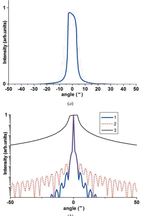
Figure 11

(a) Rocking curves for the Ge(220) collimator/monochromator crystal in the case of a single reflection (curve 1), a triple-bounce design (curve 2) and a four-bounce design (curve 3). (b) RSM (on a logarithmic scale with a step size of 0.18 for intensity, where red and blue correspond to the highest and lowest intensity, respectively) of the instrumental function for a four-bounce Ge(220) monochromator and a three-bounce Ge(220) analyser crystal. M and A are the monochromator and analyser pseudo-peaks, respectively.

Figure 12

The simulated RSMs (on a logarithmic scale with a step size of 0.18 for intensity, where red and blue correspond to the highest and lowest intensity, respectively) with the impact of the instrumental function for differentlðinÞ

parameters of the monochromator (M) and analyser (A) crystals: M;A_{ð!Þ ¼ ½ð2a}M;A

0 þÞ 2

4aMh;Aa

M;A h

1=2

, M;A 1;2 ð!Þ ¼

½M;A_{ð!Þ=2 and ¼4cos}M;A

B !=. Here ! is the

angular deviation from the appropriate Bragg angular posi-tion, the coefficients aM;A

0;h;h are equivalent to the coefficients a0;h;h in equation (1), and

M;A

B are the Bragg angles for the

monochromator and the analyser crystals, respectively. Using equation (26) we can analyse the impact of the instrumental function on the formation of RSMs. In our simulations we use a Ge(220) four-bounce monochromator crystal and a Ge(220) triple-bounce analyser crystal. The rocking curves for the Ge(220) triple-bounce and four-bounce crystals and the RSM of the instrumental function are shown in Fig. 11.

Fig. 12 shows RSMs, simulated with the impact of the instrumental function, for the different lateral sizes of the incident beam lðinÞ

x on the top surface of the investigated crystal. Fig. 6 shows these RSMs simulated without the impact of the instrumental function. The small lateral size of the

incident beam (Fig. 12a) causes a blurred intensity distribution in the RSM.

An increase of the lateral width of the X-ray illuminated area narrows the diffraction pattern (Figs. 12band 12c). The inclined strips on the RSMs are the result of the superposition of two effects: the finite width of the incident beam (see Fig. 6) and the analyser pseudo-peak. The four-bounce mono-chromator pseudo-peak is practically non-observable on the RSMs.

Fig. 12(d) shows the RSM simulated with the impact of the instrumental function in the case of an indefinitely wide X-ray incident beam. Short streaks of the monochromator and analyser crystal pseudo-peaks are observed, due to the effect of the instrumental function. Without the instrumental func-tion effects, only the main peak would be observable (Punegov et al., 2016).

The qx andqz cross sections of RSMs calculated for the different lðinÞ

x while accounting for the instrumental function are shown in Fig. 13.

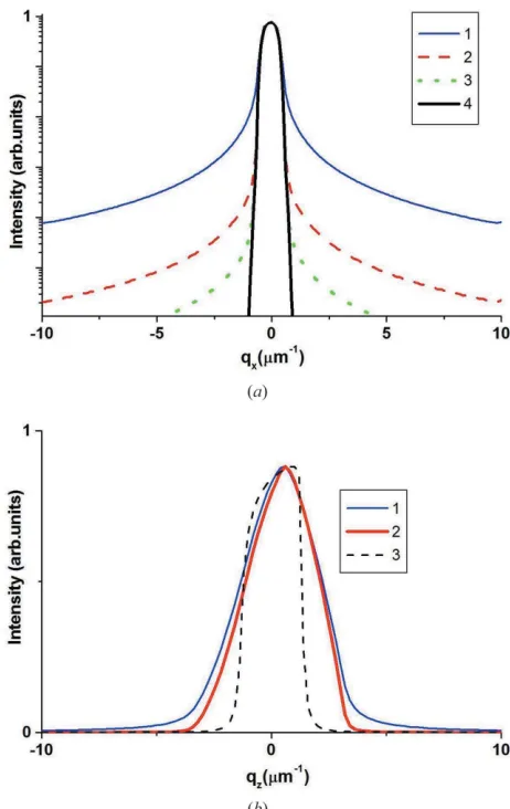
The extent and intensity of the qx cross-section ‘tails’ depend on the lateral width of the incident radiation: the wider the incident beam, the weaker the intensity of the ‘tails’. In the case of the unrestricted plane incident wave the ‘tails’ are absent (Fig. 13a, curve 4). The instrumental function extends theqzcross section and changes its shape [compare in Fig. 13(b) curves 1 and 2 and the Darwin curve 3). Unlike the qxcross section, the width of the incident beam does not affect the shape of the qz cross section, with hardly noticeable distinctions existing for the spatially unrestricted plane inci-dent X-ray wave (Fig. 13b, curve 2).

6. Concluding remarks

The developed approach allows one to correctly simulate RSMs and their cross sections for perfect crystals. Up to the present only RSMs of diffuse scattering were usually simu-lated, because the coherent component was typically calcu-lated as a function (Kaganeret al., 1997) in the case of the laterally unrestricted incident plane wave. This prevented the quantitative analysis of both the coherent and diffuse scat-tering components. The developed approach will be applicable for X-ray or neutron optics as well as for the optics of photonic and liquid crystals. This approach will also be useful for coherent diffraction imaging techniques (Pavlovet al., 2017).

It should be emphasized that the developed approach to the theory of dynamical X-ray diffraction is more general than the existing approaches because it takes into account the spatially restricted X-ray beams that are used in all real experiments. This approach may be developed further by extending the statistical dynamical diffraction theory to the case of the spatially restricted beams. This will allow one to correctly calculate intensities of the coherent and diffuse scattered waves.

Funding information

VIP and AVK acknowledge financial support from the Russian Foundation for Basic Research (projects No. 16-43-Figure 13

(a) Simulated qx cross sections of RSMs with the impact of the instrumental function, with lðinÞ

x of 30mm (curve 1), 300mm (curve 2), 900mm (curve 3) and1(curve 4). (b) Calculatedqzcross sections of RSMs with the impact of the instrumental function forlðinÞ

x of 30mm, 300mm and 900mm (curve 1, curves are indistinguishable); forlðinÞ

x =1 (curve 2); and for alllðinÞ

110350, No. 17-02-00090) and the Ural branch of the Russian Academy of Sciences (project No. 15-9-1-13). KMP acknowl-edges financial support from the University of New England.

References

Authier, A. (2001).Dynamical Theory of X-ray Diffraction.Oxford

University Press.

Berenson, R. (1989).Phys. Rev. B,40, 20–28.

Bhagavannarayana, G. & Zaumseil, P. (1997).J. Appl. Phys.82, 1172–

1177.

Boulle, A., Masson, O., Guinebretie`re, R., Lecomte, A. & Dauger, A.

(2002).J. Appl. Cryst.35, 606–614.

Bushuev, V. A. (1998). Dynamical Diffraction of Bounded X-ray

Beams. Preprint of the Physics Department of Moscow State University, No. 14/1998, pp. 1–12.

Bushuev, V. A. & Oreshko, A. P. (2007). J. Surf. Invest. X-ray

Synchrotron Neutron Tech.1, 21–27.

Faleev, N. N., Honsberg, C. & Punegov, V. I. (2013).J. Appl. Phys.113,

163506.

Fewster, P. F. (1989).J. Appl. Cryst.22, 64–69.

Gartstein, E., Mandelbrot, M. & Mogilyanski, D. (2001).J. Phys. D

Appl. Phys.34, A57–A63.

Ha¨rtwig, J. (2001).J. Phys. D Appl. Phys.34, A70–A77.

Holy´, V. & Mikulı´k, P. (1996). X-ray and Neutron Dynamical

Diffraction Theory and Applications, NATO ASI Series, Vol. 357, edited by A. Authier, S. Lagomarsino & B. K. Tanner, pp. 259–268. New York: Plenum Press.

Iida, A. & Kohra, K. (1979).Phys. Status Solidi (A),51, 533–542.

Irzhak, D. V., Knyasev, M. A., Punegov, V. I. & Roshchupkin, D. V.

(2015).J. Appl. Cryst.48, 1159–1164.

Jergel, M., Mikulı´k, P., Majkova´, E., Luby, Sˇ., Sendera´k, R., Pincˇı´k, E.,

Brunel, M., Hudek, P., Kosticˇ, I. & Konecˇnı´kova´, A. (1999).J. Appl.

Phys.85, 1225–1227.

Kaganer, V. M., Ko¨hler, R., Schmidbauer, M., Opitz, R. & Jenichen,

B. (1997).Phys. Rev. B,55, 1793–1810.

Kazimirov, A. Yu., Kovalchuk, M. V. & Kohn, V. G. (1990).Acta

Cryst.A46, 643–649.

Korn, G. A. & Korn, T. M. (1968).Mathematical Handbook. New

York: McGraw Hill Book Company.

Lomov, A. A., Punegov, V. I., Nohavica, D., Chuev, M. A., Vasiliev,

A. L. & Novikov, D. V. (2014).J. Appl. Cryst.47, 1614–1625.

Mikhalychev, A., Benediktovitch, A., Ulyanenkova, T. &

Ulya-nenkov, A. (2015).J. Appl. Cryst.48, 679–689.

Nesterets, Y. I. & Punegov, V. I. (2000).Acta Cryst.A56, 540–548.

Pavlov, K. M., Punegov, V. I., Morgan, K. S., Schmalz, G. & Paganin,

D. M. (2017).Sci. Rep.7, 1132.

Punegov, V. I. (1993).Phys. Status Solidi (A),136, 9–19.

Punegov, V. I. (2012).Tech. Phys.57, 37–43.

Punegov, V. I. (2015).Physics-Uspekhi,58, 419–445.

Punegov, V. I., Kolosov, S. I. & Pavlov, K. M. (2014).Acta Cryst.A70,

64–71.

Punegov, V. I., Kolosov, S. I. & Pavlov, K. M. (2016).J. Appl. Cryst.49,

1190–1202.

Punegov, V. I., Nesterets, Y. I. & Roshchupkin, D. V. (2010).J. Appl.

Cryst.43, 520–530.

Stepanov, S. & Forrest, R. (2008).J. Appl. Cryst.41, 958–962.

Takagi, S. (1962).Acta Cryst.15, 1311–1312.

Wei, G. W., Zhao, Y. B. & Xiang, Y. (2002).Int. J. Numer. Methods

Eng.55, 913–946.