Orbital characteristics of meteoroids

ORBITAL CHARACTERISTICS OF METEOROIDS

A thesis

submitted for the Degree of

Doctor of Philosophy in Physics in the

University of Canterbury

by

D. I. Steel

p• 1y�ICAL , - ·r' 1-�t. ,.,: CHAPTER 1 2 3 4 CONTENTS ABSTRACT INTRODUCTION

THE PROBABILITY OF AN ENCOUNTER BETWEEN TWO OBJECTS IN ARBITRARY KEPLERIAN ORBITS

2.1 Introduction

2.2 Basis of the method 2.3 Spatial density 2.4 Relative velocity 2.5 Collision probability

THE RESULT OF AN ENCOUNTER BETWEEN A MINOR BODY AND A PLANET

PAGE 1 3 10 13 15 28 32

3. 1 Introduction 3 4

3.2 Deflection producing a grazing impact 35 3.3 The sphere of influence and the

'minimum deflection' 38

3.4 The mean and root-mean-square

deflections in an encounter 39

3.5 Probability of ejection 43

3.6 Orbital energy change per encounter 51

FACTORS LIMITING THE LIFETIMES OF METEOROIDS

4.1 Introduction

4.2 Sporadic meteor production 4.3 Radiative forces on meteoroids 4.4 Lorentz scattering

4.5 Rotational effects

4.6 Inter-particle collisions 4.7 Surrunary

CHAPTER

5

6

7

8

PLANETARY DISRUPTION OF METEOROID ORBITS

5.1 Introduction 5.2 Results

5.3 Discussion

COMPARISON OF THE VARIOUS METEOROID LIFETIMES

6.1 Presentation of the data 6.2 Deductions

6. 3 Summary

APPLICATION TO OTHER SOLAR SYSTEM SCENARIOS

7.1 Introduction

7.2 Hidalgo and Chiron

7.3 Other asteroids which cross the giant planets

7.4 Neptune and Pluto

CONCLUSIONS

ACKNOWLEDGEMENTS

REFERENCES

APPENDICES

PAGE

84 87 104

109 110 116

117 118

124 128

135

139

140

1 Planetary encounter program 150

2 Asteroid collisions with the terrestrial

FIGURE 1

FIGURE 2

FIGURE 3

LIST OF FIGURES

The variation of spatial density with distance from the primary

The variation of spatial density with ecliptic latitude

Relative velocity of the two colliding objects

FIGURES 4a & 4b Pre- and post-encounter geometry

FIGURE 5

FIGURE 6

FIGURE 7

Deflection in an encounter, and the escape cone

Lifetimes for various stream orbits

Variation of the collisional lifetime of Zagreus with semi-major axis

PAGE

16

21

30

45

46

113

TABLE 1

TABLE 2

TABLE 3

TABLE 4

TABLE 5

TABLE 6

TABLE 7

LIST OF TABLES

Collisional lifetimes of 1 mm meteoroids in various orbits

Orbits, masses and radii of the planets

The effects of close planetary encounters upon test orbits

Lifetimes for various stream orbits

Close encounters by Hidalgo and Chiron to the giant planets

Orbital parameters of four Jupiter­ crossing asteroids

Encounter probabilities with Jupiter for four asteroids

PAGE

80

85

88-103

111

122

125

1.

ABSTRACT

The bulk of meteoroidal particles follow pseudo-random orbits and are termed sporadic meteoroids. These are

thought to be derived from the correlated streams of particles released by comets, although the mechanisms by which their orbits are dispersed have been the subject of some confusion. By developing techniques to compute the frequency of close encounters with each of the planets, and also the gross

outcome of such events, it is shown that most sporadic orbits are a result of gravitational scattering by the giant planets. Jupiter plays the major role.

Although catastrophic impacts with smaller particles limit the lifetimes of meteoroids, this mechanism is not responsible for the bulk of the stream disruption. With a simple model of the zodiacal cloud, the method is also

used to find the collisional lifetime of meteoroids including for the first time the dependence upon inclination.

The rate of meteoroid depletion by planetary collisions and hyperbolic ejections resulting from close approaches is calculated. It is found that for Jupiter-crossing meteoroids these losses are as rapid as those due to the Poynting­

Robertson effect.

This theory is also applied to six peculiar asteroids, including Hidalgo and Chiron. These prove to have extremely short-lived orbits: large orbital variations occur on a time­ scale of only �103 years. It is also shown that Pluto

2 •

The collision rate between the Apollo-Amor-Aten

asteroids and each of the terrestrial planets is calculated using all 7 6 known objects. The result using this new

procedure (4- 6 Earth impacts per million years ) is somewhat higher than previous estimates, indicating that these

3 .

CHAPTER 1

INTRODUCTION

In this thesis I investigate the role of close

planetary encounters in the evolution of the smaller bodies in the solar system: the main concern is the dispersion of meteoroid orbits, but the theory can equally well be applied to asteroids and comets.

In recent years as a result of spacecraft observations much attention has been focussed upon the dynamics of the cloud of particles responsible for the zodiacal light, the majority being particles smaller than 100 wm. A variety

of forces influence the distribution of these particles. Burns et al. (19 79) closed their review of the radiative forces at work by noting that new approaches are necessary

for evaluating the long -term effects of planetary perturbations and stochastic collisions. This is especially true for

larger interplanetary particles, upon which the radiative forces are much less important: such a new approach is developed here.

In particular I intend to deal with those particles which give rise to meteors (observed by radar, photographic, TV, visual or other techniques) when they enter the Earth's

atmosphere. These bodies, which can conveniently be

considered to range in radius from 100 wm to 1 cm, will be

denoted as m,•lcoroids although the semantically-incorrect

term mel�or is sometimes more easily used. By convention

smaller particles are often called dust and much larger

4 .

There are many outstanding problems in what might be called the ecology of interplanetary particles which have been discussed in detail in several recent books or collections of papers (e.g. Elsasser and Fechtig, 1976; Delsemme, 1977; McDonnell, 1978; Halliday and McIntosh, 1979; and specific references in this text). It is believed that the majority of meteoroids are particles released by comets whilst passing through the inner solar system, and that these replenish the

zodiacal light cloud when fragmented in catastrophic collisions. Nevertheless there are major problems of understanding in

each of these two steps and much observational and modelling

work still remains to be done. The mass distribution index

for different populations is an important indicator as to the processes which are occurring: this is reviewed by Hughes

(1978) but is not touched upon here.

After release a meteoroid follows an orbit similar to its parent comet since their relative velocity is small. This results in a stream of particles, and hence the meteor showers seen on the Earth at various times of the year.

However only �25% of all meteors are associated with streams,

the rest comprising a pseudo-random influx of sporadic

meteors. The mechanism whereby meteoroids are thrown

from their original streams into dissimilar sporadic orbits is another major problem in meteoroid ecology, as was

explicitly stated by Dohnanyi (1970; p.3485). Important

questions still to be answered for meteoroids are the same

5.

magnitude of these perturbations and what are the associated

time-scales? How far is the gravitational sphere of

influence of each of the planets? Does Mercury affect the

dust distribution despite its small mass? " These are

the questions which I have attempted to answer in this thesis . The confusion in this area is well-illustrated by the fact that, in two chapters in the same volume, Dohnanyi (1978) ascribes sporadic production to the scattering of stream

meteoroids by the planets (as was first suggested by Plavec in 1956) whilst Hughes (1978) states that sporadics are largely the result of collisions between stream meteoroids and zodiacal cloud particles. Although it has been known since the work of Zook and Berg in 1975 that the eventual fate of a meteoroid is most likely a catastrophic impact, and also the high mass index of sporadics shows that collisions must play some part, it is by no means clear that the

majority of sporadics originate in meteoroid-dust collisions. To date there has been no quantitative footing to ideas upon the providence of sporadic meteor orbits, which are totally different to those of comet-associated streams (e.g. Hawkins, 1962).

A number of different approaches have been used to investigate the orbital characteristics of the smaller bodies in the solar system. Concentrating upon the origin of

meteorites, Arnold (1964, 1965) used an encounter probability method coupled with a Monte Carlo simulation of the outcome

of close encounters. Other Monte Carlo simulations, or

variants, have been used in studies of the origin of asteroids and comets (Everhart, 1968; 1969; 1972; 1973;

19 80b; Rickman and Froeschle, 1980), although these require

vast amounts of computing time. Kresak (1982) has

6.

discussed the use of the Tisserand invariant (Jacobi constant) and the D-criterion (described in chapter 4) in differentiating

between cometary , asteroidal and meteoroidal orbits. Alfven

and Arrhenius (19 7 6) have put forward many novel ideas upon

the interrelation of meteoroids and comets, and have discussed

the origin of sporadic orbits in general terms. Despite the

above advances there has been no definitive answer to the origin of sporadic orbits since Plavec (1956) suggested

the dispersion of meteor streams by planetary close encounters. Recently some work has been done upon exact calculations of close encounters between specific streams and Jupiter

(Carusi et al. 1981; 1982a; 1982 b; 1983). The results show that the stream is destroy ed by the encounter, and the stream

particles are dispersed into the sporadic background. However,

this is for a particular case only,where the meteoroid

trajectories are chosen so as to intersect the planet. To

find the gross effect of planetary encounters the probability (or frequency) of such encounters is required, and also some measure of the outcome of these events: these factors I

evaluate as follows.

The first step is to deduce the frequency of meetings between a particle in an arbitrary orbit and each of the

planets. The technique used to accomplish this, detailed

in chapter 2, is due to Kessler (1981). This method was preferred, rather than the limited methods based upon the work of Opik (1951; 19 7 6) which have been in favour to date, because the relative velocity and encounter geometry of

7 •

situations. These parameters are needed in the second step,

described in chapter 3, which involves calculating the

partition between the different outcomes of such an encounter (i.e. collision with the planet, ejection from the solar

system, or a perturbation of the original elliptical orbit). A computer program which performs these calculations is

included as Appendix 1.

Use of this program to find the sporadic production rate is discussed in chapter 4; the time-scale for sporadic production must be compared to the time-scales for the other

dynamical effects which are also reviewed there. It is

confirmed that the limiting lifetime for meteoroids is

defined by impacts with zodiacal cloud particles. The

techniques of chapter 2 are also used to make a new deduction of the meteor collisional lifetime using a simple model of the zodiacal cloud based upon spacecraft measurements, the

results confirming previous rudimentary estimates. This

is the first time that the dependence of the inclination of the meteoroid orbit has been included in the calculation

(c.f. Leinert et al, 1983) and is therefore a significant improvement upon previous methods.

Many of the factors influencing the lifetimes discussed in chapter 4 are dependent upon the meteoroid density. There is now a wealth of evidence that whilst the smaller particles (e.g. 1-100 µm dust, the dynamics of which were investigated

by Kresak, 1976) have densities of 3-4 gm cm-3

(Hanner, 1980), meteoroids have a much lower density in line with a looser

structure (Hughes, 1978). The densities measured by radar

techniques show a large scatter but a value of �0.8 gm cm-3

have put forward a theory to explain how gradual closer packing of a meteoroid can slowly increase its density. In view of the above, and for the sake of simplicity, I shall

-3

adopt a mean density of 1 gm cm throughout.

Attention is next turned to meteoroid losses caused

8

by the planets (planetary impact or ejection on an hyperbolic orbit), and sporadic meteoroid production in close encounters. The results for a wide variety of sample orbits are calculated in chapter 5, and in chapter 6 the important time-scales are calculated for each distinct set of orbital elements. A number of new and important deductions are made, the most significant being:

a) Meteoroids in Jupiter-crossing orbits suffer losses

due to planetary collisions and (more abundant) ejections

at a rate comparable to depletion by the Poynting-Robertson effect;

b) Jupiter-crossing stream meteoroids are dispersed into

sporadic orbits by close encounters much faster than they are lost from the meteoric complex .

As aforementioned, the theory developed here can also be applied to larger bodies. In chapter 7 I investigate the orbital evolution of several objects of particular interest: the two giant asteroids Hidalgo and Chiron, each of which crosses two of the giant planets, and four smaller asteroids which cross Jupiter. All six are shown to have

lifetimes in their present orbits which are extremely brief

compared to the age of the solar system. Only one planet

9.

The meteoroid orbits used in chapter 5 are typical

of a variety of comets. For the sake of brevity I do not

additionally consider any specific comets, although it is noteworthy that the evolution of cometary orbits can also be

researched using these techniques. In particular, the

principle of reversibility implies that the ejection probabilities calculated for the closed orbits used here are upper limits for the capture probabilities of hyperbolic

comets entering the solar system. The amount of computation is modest compared to the Monte Carlo simulations of comet capture carried out by Everhart (1969; 1973), and others.

There is one other category of interplanetary particle which is of much interest: the Apollo-Amor-Aten asteroids,

which cross the terrestrial planets. These are removed

quickly due to planetary impacts, and the necessary supply has been the subject of intense study over the past decade. In Appendix 2, consisting of a substantial paper which has been accepted for publication, I re-evaluate the collisional lifetimes of these objects using the new techniques

embodied by this thesis. The results allow a prediction of

the cratering rate on Mercury, Venus, the Earth and Mars in

the present epoch. Comparison with the long-term lunar

CHAPTER 2

THE PROBABILITY OF AN ENCOUNTER BETWEEN TWO OBJECTS IN ARBITRARY KEPLERIAN ORBITS

2.1 INTRODUCTION

10.

In this chapter I derive the probability of an

encounter between two arbitrary orbiting objects, expanding

upon the description of Kessler (1981). This method is

easily implemented by computer. Distinct methods have been

II

those of Opik (1951), Wetherill (1967), and Shoemaker et al. (1979)

11

Opik (1951) developed an approximate theory for

calculating the probability of an impact by a minor body in an elliptic orbit upon a planet in an orbit taken to be

II

circular. This was applied by Opik to a number of particular

11

objects in the solar system (Opik, 1963, 1966a; and numerous

other papers). The limitations imposed by the approximations

11

made have been discussed (Opik, 1976).

Wetherill (1967) derived a more general set of equations by allowing both objects to be in non-circular orbits, thus deriving a more complex but more precise formalism which he applied to the problem of collisions in the asteroid belt.

Shoemaker et al. (1979) used a similar but alternate derivation to that of Wetherill in order to estimate the

asteroidal collision rate with the Earth. Their method is useful in that it incorporates the secular perturbations

which alter the orbits of the objects in question, whereas

1 1

Thus Kessler's equations give a zero impact probability with the Earth for an Amor asteroid, since it is not

presently an Earth-crosser, whereas secular variations may change it into an Earth-crossing (Apollo) asteroid eventually, with a finite collision probability. However, an exact

solution to the equations of Shoemaker et al. (1979) is not yet possible, severely limiting their application .

Recently Greenberg (1982) has derived a new geometrical formalism for orbital encounters avoiding many of the

II

approximations of Opik and Wetherill . With some refinement it may be possible to extend Greenberg's method to include the effects of secular perturbations, and to find the gross

effects of close encounters . (e . g . to calculate the probability of ejection from the solar system by a different technique

to that described in chapter 3).

In this chapter it is assumed that the type of event in question is an actual impact, so that the collision cross­ section is the cross-section of interest (equation 2) . In chapter 3 the cross-sections for deflection, ejection, and collision, are all derived. Thus to find the probability of an ejection or deflection it is simply necessary to replace

a.

Kessler's method is analogous to the kinetic theory of gases. The orbit of each object is described by semi-major axis a, eccentricity e, and inclination i. An essential feature of the method is that the argument of

II

12.

method, as presented in the later chapters of this thesis, show that close encounters producing deflections of a few degrees occur for planet-crossing objects on time-scales of

6

10 years or less. Smaller deviations will be very much more frequent, and time-scales of 104-105 _{or less years are}

applicable to minor changes in a particle's orbit due to

planetary perturbations which cause an appreciable alteration of the argument of periapsis. The argument of periapsis

(or the longitude of periapsis and the longitude of the node) is hence essentially random, and Kessler's method is valid. An exception to this would be a particle whose orbit was 'protected' by being 1n some form of resonance with a planet

(e.g. the Trojan or the Hilda asteroids). Such a resonance is generally possible if the minor body crosses one planet only. For example, the resonance which prevents Toro from striking the Earth is not stable since this asteroid crosses Mars also (Shoemaker et al., 1979).

The collision probability for two secondary bodies orbiting a given primary object is a function of the

two sets of orbital elements (a, e, i), and the physical characteristics of these bodies (mass and radius, m and r). Therefore, with M the mass of the primary, the collision probability over a long time-base with random argument of periapsis is:

This technique is especially valuable in dealing

13.

can be used for any Keplerian orbits, such as stars about the centre of their galaxy, or moons orbiting their parent

planet . The method was developed to find the collisional lifetime of artificial satellites in Earth-orbit by Kessler

and Cour-Palais (1978), and was applied by Kessler (1981) to the outer moons of Jupiter

2 . 2 BASIS OF THE METHOD

Take the volume of space in which it is possible for the two objects to collide to be split up into small volume elements �U, each of which is small compared to the

uncertainty in the orbital paths of the objects . Then the positions of each object within any volume element 1s essentially random, as are the molecules in a gas, and the flux of one object is

F Sv

where v is the velocity of the object, and S its mean 'spatial density' within the volume �U; that is, inside of this volume element there are on average s bodies having this orbit, per unit volume.

( 1)

The number of impacts upon an area A in time t is then given simply by FAt . However, in general the objects have an appreciable gravitational field so that gravitational focussing increases the effective collisional cross-section

II

( 2)

In the case of a minor body such as a comet or asteroid

striking a planet, r2 and m2 are small. Then the term

outside of the bracket is just the geometrical cross­ section of the planet, and the inside of the bracket is unity plus the ratio of the square of the planetary

escape velocity to the square of the encounter velocity,

v.

The number of collisions in time t 1s then

N = Fot

so that the collision rate is, from (1 ) and (3 ) ,

N _{= Svo} t

However, this would assume that one body is held stationary in the volume element; in fact there 1s only a small chance that both objects will be in the volume element at the same time, so that (4) becomes

( 3)

( 4)

( 5) 14.

where S1 and S2 are the respective spatial densities of the two objects in this particular volume element 6U,

The total collision probability between the two is the sum of the collision rates in all volume elements accessible to both objects:

p = I S1S2VO dU

volume ( 6)

This assumes that the collision probability is sufficiently small such that many orbits are executed. Equation ( 6 ) can be solved numerically by defining volume elements of such a size that the spatial density does not vary appreciably within the element; then

a . 6U.

J J ( 7)

where the bars indicate that the mean value throughout the element is used.

15.

Once the mean encounter velocity is known (section 2.4), the collision cross-section can be calculated from equation (2). In section 2. 3 the expression for the spatial density is deduced.

2.3 SPATIAL DENSITY

If the argument of periapsis is random, then the spatial density is a function of distance to primary (R ) and ecliptic latitude (B) only, so that

-

_---

_-

ORBIT

FIGURE 1

SHELL OF

THICKNESS �R

16.

In addition, Sis separately dependent upon these two parameters:

S(R, B) = Q(R)B(B) ( 8)

Here Q is the spatial density at R averaged over all latitudes, and Bis the ratio of the spatial density at B to the spatial density averaged over all latitudes. Q depends upon the size and shape of the orbit, described by a and e; or equally well by periapsis distance q and apoapsis distance q':

Q(r)

=

=

B depends only upon the inclination:

B(B) = B(i)

and the two functions Q and B are derived separately.

2. 3. 1 Radial Spatial Density Variation

Consider a spherical shell of thickness 6R, at a distance R from the primary such that (q � R � q'), as in Figure 1.

The orbiting body has a velocity VB with radial component

V = V sin y _{r B ( 9)}

V is taken to be positive towards the primary so _r

that from apoapsis to periapsis (0° _{� y � 90}°_{), and from}

periapsis to apoapsis (2 70° _{� y � 0}°_{). The shell has an}

internal distance R, external distance R', mean distance

R = (R + R')/2

and a volume

18.

( 10)

as long as (6R << R).

In each orbit the body passes through the shell twice, so that the time spent within the shell per orbit is

6t = 26R/V r

The velocity of the body is

G being the universal constant of gravitation.

Equations (9) and (12) will allow 6t to be calculated from (11) as long as sin y is known.

The angular momentum per unit mass is:

(11)

(12)

at q'

at R

or

q'V cos0°

Bq' = q'VBq'

RVBR cosy = [GM[¾ -

¼Jf

Equating (A), (B) and (C) gives

2q - q2_{/a = 2q' - q'}2_{/a =}

[¾ -

¼)

cos2_{y = 2qa-q}2 _ 2q'a-q'2 R ( 2a-R) - R ( 2a-R)

However,

a= (q+q')/2 so that

qq' = 2qa - q2 _{= 2q'a - q'2}

and then

cos2_{y =} qq' R ( 2a-R)

Since sin2_{y = 1 - cos}2_{y, equations (9), (11) and}

( 12) give:

The spatial density is just

Q = .6t/T.6U

where the period T is

J..: T = 2 TI ( a 3 /GM) 2

19.

( B)

( C)

(13)

(14)

( 15)

and then (10), (14), (15) and (16) render

Q(R) - l/4nR2_aJ,

[[¾ - ¼]

)r

which, with substitution of a = (q+q')/2,gives

k Q ( R) = 1 / 4 n 2 _{Ra [ ( R-q) ( q' -R) ]} 2

20.

( 1 7)

This is the probability of finding the body within a shell of unit volume at distance R, averaged over all latitudes. For (R < q) or (R > q'), Q = O. The method for dealing with Q as (R � q) or (R � q') is dealt with in section 2. 3. 5.

2. 3. 2 Latitudinal Spatial Density Variation

The orbiting body is now defined to be within a

shell of thickness 6R at distance R. The requirement is to find the probability of finding the body within a band of latitude from B to B + 66.

Referring to Figure 2 , XY is the ecliptic plane. The body is imagined to be held stationary at the point

o,

that it traverses path WOX. All possible values for the argument of periapsis of the real orbit are scanned in this way.

21.

z

y

X

FIGURE 2

22.

circular, then the period of this imaginary orbit is

T' = 2rr/w (18)

The time taken to cross the latitude band of width 6B is just (6B/wsina) where a is the angle which the path makes with the line of constant latitude. Since the object crosses this latitude twice in every orbit, the total time spent in this band per orbit is

6t' = _26B/wsina (19)

Equations (18) and (19) therefore give the fraction of the object's time spent between Band B+6B as

6t' ₌

T' rrsina (20)

In a similar way to ( 15) , since we need to consider a unit volume given by eauation (10),

B _{= 6t'/T'6U'}

and 6U' is required in order to calculate B.

The volume of a hemispherical shell is (2rrR2_6R),

and the volume element decreases as the cosine of the latitude. Thus

AU' = 2rrR2 _{cosB 6R6R}

and putting (20) and (22) into (21) renders:

B _{= l/2n2R2sina cosB 6R}

or

(21)

23.

B = 2/n sina cosB (23)

which is valid for 0° _{( B � i; B = 0 at higher latitudes.}

Since

cosi = cosa cosB

so that

sina cosB

and hence

k

= _[sin2_{i - sin}2_B] 2

k

B (B) = 2/n[sin2_{i - sin}2_B] 2 _{( 24)}

Treatment of this equation as (B � i) is described in section 2.3.6.

2. 3. 3 Net Spatial Density Variation

Equations (17) and (24) can now be substituted into

(8) to give the net spatial density. Since R and Bare better measures than R and B, write

S (R,R' ,B,B') = l/2n3_{aR[ (sin}2_i-sin2_{S) (R-q) (q'-R)]} ½

which is valid for

and

( q � R' R I (; q I )

(0° _{( IB,B'I (; i)}

The spatial density is zero outside of these limits, but care must be taken as these limits are approached.

2 .3 .4 Integration Methods

The singularities ocurring when (R + q ) , (R + q '), or (B + i ) are integrable as follows. The average spatial density within a volume is

24.

S = f Sdu/f dU (26 )

which must be separated into radial and latitudinal terms. For very small volume elements equation (22) is

dU = 2 nR2 cos B dR dB

and thus using (8) equation (26 ) becomes

- _{ff Q (R)B(B ) R}2 _{cosB dR dB}

s =

ff R2cos6 dRdB

Since Rand B are independent, the integrals are separable:

S(R,R',B,B') = Q(R,R') B(B,B ')

Here

R' R'

Q(R,R') = f Q(R)R2_{dR/f R}2_dR

R R

(27)

(2 8)

(2 9)

25.

B'

B'

B (B,B') = J

B B (B) cosB dS/f B cosB dB (30 ) is the ratio of the mean spatial density between B and B' to the mean spatial density over all latitudes.

Solutions to equations (29 ) and (30 ) now are required.

2. 3. 5 S patial Density as (R�q) or (R�q')

Let the thickness of the spherical shell (6R) be sufficiently small such that the radial distance at any point can just be set to the average radius:

and

R' R'

J

R R2Q(R)dR � R2 f R Q (R) dR

Thus (29 ) becomes

R'

Q (R,R') =

6; JR S (R)dR

and by substituting (17 ) this is

Q(R,R') = _{[ ( R -q ) ( q} 1 -!-:

-R) ] 2 d R

After evaluation of the integral this becomes

Q(R,R') = 1 [ arcsin . [2R'-2al

which is valid for all volume elements entirely outside of the periapsis (R > q) and inside apoapsis (R' < q').

If (R � q) then the square bracket becomes

. (2R' -2a} TT [arcsin q'-q + 2J

if (R' � q ') then the square bracket becomes

[TT _{2 - arcsin q'-q} . [2R -2a}J

if (R > q') or (R ' < q) then

Q(R,R') = 0.

For an extremely low eccentricity orbit it is possible that both (R � q) and (R' � q '), in which case the square bracket is just TT, and equation (31) is then

Q (R, R') = l/4TTaR6R

However, since q and q' are effectively the limits of R and R', and a = (q+q')/2 = R here, this becomes

Q(R � q,R' � q') = l/4 TTR26R

It shoulr be noted that the equivalent to this in Kessler (1981) (equation llA) contained a typographical error. His equation lOA should also have been for the

27.

mean spatial density (Kessler, 1984 , personal communication ).

A numerical comparison of the results of equations

(29) and (31 ) shows that the approximation used in deriving

(3 1 ) leads to a typical error of 0. 3% for a thousand-point

summation in place of the true integral.

2.3.6 S patial Density as (8 + i )

A solution to equation (30 ) is required. The value

of the denominator is simply (sin8' - sin8 ), but the

numerator is more complicated. Using equation (24 ) the

numerator is

8 1 81

J

S B(S )cosS d8 =

Is

2 cos 8

½ n[sin2i - sin28]

cosS _d8

[ l

-= 2 [arcsi_1T n(s�_Slnl n�'} - arcsin(s�_Slnl n�JJ

Thus equation (30 ) becomes

d8

B(B,8' ) = __{TI_(_s-1-. n-8-�---s-1-. n-S- ) [ arcs i}n (

:t��

(3 2 ) This is the average spatial density between latitudes

8 and 8' compared to the spatial density averaged over all latitudes.

(sin (6 or 6')/sin i) cannot exceed unity. Therefore when (8' � i) or (-6 � i) the relevant arcsine takes the value (n/2). If ( 6 � i) or ( -6 ' � i) , B ( 6, 6 ' ) = 0 .

It is easily seen that since 8' > B always, the factor outside of the bracket ensures that the calculated spatial density is positive.

2.3. 7 Overall Spatial Density

28.

Equations (31) and (32) can now be substituted into (28) to give the mean spatial density between radial distances R and R ' and between latitudes 6 and 6':

S (R, R ',6,6 ')

1

=

2n3_{aR6R (sin6'-sin6)} [

· 2R 1 -2a

l

r •

l

arcsin ( , _{q -q} ) arcs in ( . . ) _Slnl

. 2R-2a

l .

-arcsin ( , _{q -q} ) -arcsin (-.-.) _Slnl

( 3 3) This formula is necessary when R or R' are close to periapsis or apoapsis; and when the absolute values of the latitudes 6 or B' are close to the inclination of the orbit. Otherwise equation (25) is used to find the spatial density.

2. 4 RELATIVE VELOCITY

equation (12), and then the relative velocity from

as long as the encounter angle� is known. Figure 3 represents a coordinate system centred upon the point

29 .

(34)

of intersection, with the XY plane perpendicular to the spherical shell in Figure 1. The angle� can be calculated by spherical trigonometry as:

The values of cos Y1 and cos y2 are given by equation (13), taking the positive square root in each case since (270° _{� y � 90}°_{). Hence siny1 and siny2 can}

be calculated, but these can take either sign: from apoapsis to periapsis (0° _{� y � 90}°_{) so that siny is}

positive. From periapsis to apoapsis the converse is true.

In considering Figure 2 it was seen that

cosi = cosa cosB

(35)

so that a1 and a2 can be calculated from the inclination and the latitude:

cosa = cosi/cosB ( 3 6)

30.

z

INTERSECTION

POINT

"'����

====

t===r;

y

_y

TO PRIMARY

FIGURE 3

6

Since 270° _{� a � 90}° _{, cosa is positive. However,}

(a1-a2) can take any value so that cos (a1-a2) can be positive or negative.

31.

It is seen therefore that each of the square brackets in equation (35) can be positive or negative, and four

values for intersection angle � are possible in any particular volume element:

cos� = ±[siny1 siny2] + [cosy1 cosy2 cos (a1 ± a2)]

( 3 7)

Hence there are four possible intersection velocities

resulting from equation (34). For the purposes of calculating the mean collision probability via equation (7), the mean

encounter velocity is required: this is just the average of the four possible collision velocities. However, as was made clear by Kessler (1981), this is not the same as saying that all collision velocities are equally likely:

the higher velocities render a higher likelihood of

collision. (An exception to this is when a minor body

encounters one of the giant planets: the enhancement of the gravitational cross-section over the geometrical cross-section, given by equation (2), depends upon the

2. 5 COLLISION PROBABILITY

All terms are now available for the evaluation of equation (7). The two spatial densities S1 and S2 are

given by (25) or (33), bearing in mind the limitations of validity given after equation (25). The mean velocity is found from (34) using (37) and the mean radius vector R fran (12). The collision cross-section is calculated from

(2) using the mean relative velocity. Finally the

volume element is given by (22) with the mean parameters being used; i. e.

32.

6U = 2nR2 cos B 6R 68 (38)

Equation (7) can now be numerically integrated. This must involve a compromise between precision and the computation time involved. However, since an exact collision probability lacks physical usefulness, a precision of better than 1% is not required. In fact the assumptions and approximations made above do not warrant more exact computation. An error limit of 10% is entirely satisfactory.

Kessler (19 81) used a radial jump of 6R � O.lR,

producing an error of less than 1% in the radial dependence (c. f. section A. 3. 5). His latitude bands were 68 = 3°_.

It was found here that 100 iterations in radius (6R = 0.0 1 R at worst) and 50 iterations in latitude (68 = 3�6 at worst) is sufficiently precise for all orbits, bearing in mind

investigate the volume of space accessible to both bodies and then subdivide this into a suitable number of volume

elements by defining 6R and 6B). The summation of (7)

is then over this number of volume elements, j.

A word of warning to future computors: ensure that the volume elements straddle (R = q, q') and (B = 0°_{, ±i).}

CHAPTER 3

THE RESULT OF AN ENCOUNTER BETWEEN A MINOR BODY AND A PLANET

3. 1 INTRODUCTION

34.

In this chapter I show how an estimate can be made of the result of a close encounter between a body of negligible mass (e. g . a comet , asteroid or meteoroid ) and one of the

planets. The general method used here is a development

of the techniques described by Weidenschilling (1 975 a ) , and also by Fernandez (19 7 8).

The result of a close encounter can be an ejection from the solar system , an orbital disruption , or a collision

with the planet . I refer to these respectively as being

an ej ection , deflection , or collision , and the cross-section for each of these events is required for use in equat ion (7 ) .

An exact analytical solut ion for the path taken by the minor body , hereafter termed the 'part icle ', is not possible;

this is the classic 'three-body problem '. A number of

alternat ive appro aches have been used , and mostly the

encounter is considered as being separable into two distinct

two-body phases . Outside of the 'sphere of influence '

of the planet (defined later in this chapter ) the particle mot ion is cons idered to be governed solely by the attract ion of the Sun , whilst inside this region the particle 's path

is taken to be a planetocentric hyperbola . This simplist ic

35.

points to the sphere of influence, only its direction is

changed. This separation into two, two-body problems has

II

been used extensively by Opik (19 6 6 b), Bandermann and

Wolstencroft (19 70, 197 1), Weidenschilling (19 7 5 a,b), Cox et al. (1978) and Fernandez (1978) . For very low

encounter velocities this assumption breaks down (Dole, 1962; Giuli, 1968), but is of minor importance here. As might be expected, exact numerical integrations of the orbits of minor bodies close to a planet with full consideration of the solar field indicate that the approach used here (two distinct two-body problems) does not allow an exact

prediction of the outcome of particular encounters (Carusi and Pozzi, 1978 a,b). This is because the mid-range

perturbations, outside of the sphere of influence, are not negligible. However my intention is only to find

approximate values for the probabilities of collision, deflection and ejection, rather than to plot exact orbital changes, so the simple basis of the treatment is entirely

j ustified.

3. 2 DEFLECTION PRODUCING A GRAZING IMPACT

Let a particle of negligible size and mass approach a planet of mass m1 and radius r . Using the two-body

approximation, at a large distance from the planet the

particle is taken to travel in a straight line with velocity

V relative to the planet (from equation 34). Let the

a linear path) be b. Let b be the impact parameter which _g

actually results in a grazing collision with the planet. This means that b is the maximum impact parameter which _g

results in a physical collision, so that nb 2 _{is the}

g

collision cross-section. I will follow Weidenschilling

(19 74) to find the value of b and hence the angular _g

deflection producing a grazing impact,

x .

36.

The attraction of the planet results in the particle having an accelerated r elative velocity VA when it reaches the surface of the planet, so that, by conservation of angular momentum,

V b = VA r . _g

If there is no resisting medium which slows the particle before the collision (that is, the radius of the planet is measured to the top of the sensible atmosphere) then the loss of potential energy of the particle will equal its gain in kinetic energy:

V 2 _A = v 2 + 2Gm1 _r

The second term on the right-hand side is the square

of the planetary escape velocity, V , and these two equations _e

can easily be re-arranged to give

b ?. = r 2 [1 + _g Ve2 ] = r2 [1 + 2Gm1 ]

V2 _rV2 ( 3 9 )

Rotational symmetry gives the collision cross-section as

0

C = nr2

V 2

37.

where oG is the geometrical cross-section of the planet. Equation (40 ) is the same as equation (2 ) for the case of a particle of negligible mass and radius.

The Rutherford Scattering formulae, normally used for the Coulombic field, can equally well be used for the Newtonian field (Landau and Lifshitz, 19 7 6 ) . Substituting in the planetary gravitational potential the Rutherford

Scattering impact parameter is:

Gm 1

b = cot (X /2)

v2 g

Equations (39 ) and (41 ) then give

-- rV2 [ 1

cot ( X / 2 ) _{g Gm1} + --2Gm 1] ½

rV2

( 41)

( 4 2)

which is the angular deflection producing a grazing impact.

For a point-mass planet, x would need to be 180°_.

g However,

for a real planet of finite size, X is less than this: _g for example, the zenith attraction well-known to meteor astronomers can have a value of up to 1 7°_.

x may be of the order of 150°_.

g

For Jupiter ,

3 . 3 THE SPHERE OF INFLUENCE AND THE 'MINIMUM DEFLECTION' 38.

Clearly there is no such thing as a ' minimum deflection ' since the deflection tends to zero as the impact parameter

becomes infinite. Here the term 'minimum deflection '

(denoted xd) is applied to the smallest deflection produced

by an encounter; an encounter is in turn defined as being a passage within the sphere of influence, of radius d . An angular deflection xd results from an encounter with impact

parameter b=d, so that again using the Rutherford Scattering formula,

xd = 2 arctan

[::!]

[x:]

and the radius of the sphere of influence , d, is required.

There have been a number of definitions used for the

sphere of influence. The ' Hill Sphere' of the planet is

the volume bounded by the Lagrangian points of the restricted

three-body problem , of radius

where R is the distance to the Sun , and

M is the mass of the Sun (Wetherill , 1980) .

This can be derived by requiring that the perturbation of the particle ' s heliocentric orbit due to the planet be equal to the solar attraction; this is not the same as requiring

that the planetary and solar attractions be equal (Ruppe, 1 9 6 6) .

Tisserand 's more thorough investigat ion (Ruppe, 19 6 6; p . 153) renders

39.

where A is the angle between the Sun-planet radius vector and the position angle of the particle relative to the planet . The bracketed term can vary from 1. 00 to 1. 15.

The definition used successively by Kislik (1964) , Radzievskii (1967) , Bandermann and Wolstencroft (197 �) , and Weidenschilling (1975 a) is:

( 4 4)

Since these definitions do not vary appreciably

(Wetherill, 1980) , the latter will be used here for ease of

comparison with previous work. By substituting (44) into

(4 3) , the minimum deflection in an encounter (xd) can now be calculated.

3. 4 THE MEAN AND ROOT-MEAN -SQUARE DEFLECTIONS IN AN ENCOUNTER

For an encounter where the planetary mass is large and the impact parameter is small, the deflection x will be large; a small relative velocity would enhance the deflection

(c. f. equation 4 1 ) . In such an encounter all memory of the

original traj ectory will be lost , excepting that the Jacobi constant (Tisserand invariant) will be conserved (e. g. Kresak , 197 9) .

However , most passages are distant , so that the angular deflection is small and the new particle orbit is not

substantially different from the original orbit. In a phase

space described by some form of heliocentric angular coordinates, multiple encounters by the particle with different planets

40.

deflection. Multiple encounters thus result in a

diffusion of the orbit until it no longer resembles the original particle orbit . The expectation value of the

square of the ultimate deflection (x ) is just the sum of the _u

squares of the individual deflections; i. e . , for i encounters,

I I

Opik (1966 b ) required that an accumulated Xu = 90° should occur for a complete ' loss of memory ' by the particle of its original orbit .

The above indicates that the mean and/or root -mean­ square deflection per encounter would be of use in describing the diffusion of a particle orbit .

these two parameters.

In this section I derive

The Rutherford Scattering differential cross-section for deviation x is:

do ( 4 5 )

(Landau and Lifshitz, 19 76; p . 53 ).

For a particular encounter the bracket is a constant,

and the trigonometric part can be integrated (formula

322 , p . 568, CRC Handbook ) to give a total cross -section as:

Equation (4 6 ) can be used to determine an alternative expression to (40 ) for the collision cross -section , as follows .

For an impact upon the planet, the minimum deflection required

is _{Xmin = Xg ,} given by ( 4 2 ) The maximum deflection

the collision cross -section is:

[ (Gm1 )

2

_{] [ _2}

ac = TI

-;;; sin (

X_{g/2) ( 4 7 )}

Substitution of the relevant planetary parameters and any required relative velocity shows that this renders

41.

the same result as found from (40) . In all numerical work

I have used (40) since it requires less computation.

A non -obvious error in Weidenschilling (1975a) should

be pointed out here . Clearly his equations (12) and (13) do

not lead to his equation (1 7) , a factor of TI being missing. Similarly , the TI is missing from his equation (18) . H owever,

this is correct since his normalised units are equivalent

to having a unit of time of (l /2TI ) times the planet 's orbital period , and a unit of area (1 / TI ) . This follows from taking the unit of length as being the planet 's semi -maj or axis , and the unit of velocity the planet 's orbital velocity. Weiden­ schilling 's equation (18 ) therefore gives an answer which is numerically correct , and for his units all is right if the factor of n is deleted from his equation (12) .

Equations (45) and (46) can now be used to calculate the probability of obtaining any angular deflection x within

an interval d x. This depends only upon the relative velocity

V for any particular planetary encounter since xd is a function

of V. _{Since xmin} = _{xd and xmax} = 180° this probability is

P (x l v) d x = dn _{0 - 2}

sin (xd/2) -1 ( 4 8)

value of d , and hence a smal ler minimum deflection Xd ' the probabil ity o f a certain large deflection per encounter i s decreased markedly . The probabi lity o f such a deflection per unit time remains constant .

The mean deflect ion ( xBAR) per encounter can now be found . This is

X g

J X do XBAR 0_nc

Xd

where one is the non-collisional cross-section:

or

o = nd 2 _{- o}

nc c

4 2 .

s ince any X � x results in a collision . This cross-section _g can be used in equation ( 7 ) to find P0 , the probability of a de flection .

After cancel lation of the constants ,

X BAR = [ sin -2 ( X d / 2 )

( 5 0 )

which can be integrated by parts (formu la 5 , p . 5 4 2 ;

formu la 3 0 8 , p . 5 6 7 ; formu la 3 2 2 , p . 5 68 , CRC Handbook ) to give :

( 5 1 )

in a

Next the root-mean -square deflection _{XRMs is derived} similar way. Since

1

rg

2 _x2 _do

XRMS 0_nc

X_d

4 3.

an equation for X�s is derived which is identical to (50 )

except that the x inside of the integral is replaced by x2 .

The equation can be integrated as before ( using additionally

formula 293 , p. 566 , CRC H andbook ) to get :

1-x_d2 sin- 2 (xd/2 )

+ 4x_{d cot (}xd/2 )

x; sin-2 (Xg/2 )

1

- 4 x _g cot (Xg/2 )

[ +B £n (sin (Xg/2 ) ) - 8 £n (sin (Xd/2 ) )J (52 )

In Weidenschilling (19 75 a ) the equivalent to this (his equation 2 7 ) contained an error .

A typical value of x_{RMS � (2 . 6 to 2 . B )}x_{d is derived.}

3. 5 PROBABILITY OF EJECTION

Using the deflection range x_{d to} x_{g it is now possible}

to calculate the probability of an encounter resulting in the particle being ejected from the solar system.

The planet is considered to be a scattering centre which is momentarily on a circular orbit of radius

R ,

At this solar distance the critical heliocentric velocity for ejection from the solar system is

so that V2 = 2V2

C 0

As discussed previously, in the encounter it is

( 5 4 )

44.

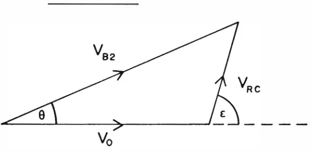
assumed that VRC ' the relative velocity of the particle and the planet taken to be on a circular orbit, is conserved in magnitude but not in direction. In Figure 4a,

v

cos 8 = cos y₂ cos (a1 ±a₂)

and VRC is given by

v

_v

_v

_{�v v}

_e

( 5 5 )

( 5 6 )

Figure 4b shows the geometry after the encounter.

A deflection x results in VRC being conserved with its

orientation changed from E to E', and thus its heliocentric

velocity is changed to v�2 . This new velocity will not in

general be in the same plane as v62 , and it is assumed that all orientations of the new relative velocity vector VRC are equally likely for a given E' (i. e. the scattering is rotationally symmetric) .

This is more clearly shown in Figure 5. A deflection x results in a new direction of VRC which may be anywhere on the circle ABCD.

VI _{>- V}

B2 r c

45 .

FI G U R E 4 a

F I G U R E 4 b

FIGURE 4

F I G U R E 5

E S CA P E

CON E

D

FI GURE 5

De f l ect ion i n an encounter , and the es cape cone

4 7 .

and this results in an 'escape cone', symmetric about the tangent, which is described by a half-angle E _C This angle

is determined by setting

vB

=

=

cos

or

= (V2 C

and any E' � E results in an ejection . _C

Similarly from Figure 4a,

( 5 7)

( 5 8)

and a deflection of at least (E - E ) is necessary for the _C

particle to attain an hyperbolic heliocentric velocity . The probability of this is now required .

Any new vector VRC which lies inside of the escape cone

will result in an ejection . In Figure 5 a particular deflect-ion x will give an ejectdeflect-ion if the new directdeflect-ion of VRC lies anywhere along the arc AB . Since it has been assumed that all orientations for a given x are equally likely, this means that the probability of an ejection in this case is just the length of arc AB divided by the perimeter of circle ABCD .

If R is the half-angle of arc AB, the probability of ejection here (i . e . the probability of an infinite heliocentric distance resulting) is:

48 .

The angle B can be calculated since the .angular lengths (E, E ,X l of its spherical triangle are known, so that: _C

or

cos B sin X sin E = cos Ec - cos X cos E

[cos E:c - cos x cos E ]

B = arcos _{sin X sin E} (60)

To get the total ejection probability for a given

encounter it is necessary to integrate P(00) over all possible deflections (all possible impact parameters). To do this

the minimum and maximum possible deflections, Xmin and Xmax' are required.

It has been seen that a deflection of at least (E -E ) _C

is needed, which would normally be the value of x . . _m1n

However, it is possible that the deflection at the edge of the sphere of influence (xdl might be greater than (E-Ec).

Therefore ,

= E -E _C

> E -E ) _C

( 6 1 )

Note that it is still possible for particles whose original orbits are near -parabolic to be ejected from the solar system although their closest approach is (b :-- d): only a very small deflection is necessary for those particles to attain a hyperbolic heliocentric orbit. Thus for particles

of large a the ejection probability derived here would be a lower limit .

This is in fact one way in which near-parabolic comets may be captured into short-period orbits by a close encounter with one of the giant planets (Everhart, 1 968 , 1 9 72, 1 9 73). S imi larly if

x

x

= E+E C ( X > g E+E ) C

4 9 .

(62) (x < E+E ) _{g C}

An additional constraint is that for some trajectories the minimum de fl ection necessary for an ejection is in fact greater than the de flection producing a graz ing impact . Equally we ll the maximum deflection producing an ejection could be less than the de flection produced at the edge of the sphere of influence. Thus for a non-zero ejection

probabi l ity it is required that:

and

Xmax > X d

( 6 3 )

Subject to (61 ,62 , 63) the probabi l ity o f ejection for a given encounter (given VRC ' E) is obtained by integrating

equation (60) over al l possible di f ferential cross-sections.

This probabi l ity is:

Xmax

p (cn_{! vRC ' E) J (}B/ n J do Xmin

50 .

! Xmax

0

µ cos ( X / 2 ) sin-3 ( X / 2 ) dx

Xmin

(64 )

with G from equation (60) .

This probability can now be used to find an ' e f fective

ej ection cross-section' , _{0 e} The encounte r cross-section is :

= nd2 _{(65 )}

and oe is defined here as:

a = ad P (00I V , E )

e RC ( 6 6 )

Equations (65 ) and (66) give cross-sections for encounter and e j ection respective ly , which can be used in

equation ( 7 ) to determine the probabi lity per unit time of these events occurring.

The integral in equation (64 ) must be evaluated

numerically . This can be performed easily using Simpson ' s

Rule , as fo l lows .

3 . 5. 1 The Ejection Integral Using Simpson ' s Rule

The integral in equation (64 ) , with G given by ( 60)

needs to be found numerically. The standard method for

performing such a quadrature is the use of Simpson ' s Rule , which is applicabl e whe re the polynomial is of the

third-degree or less. ( See , for example , Kopal , 1955 ; Conte , 1965 ;

Dorn and McC racken , 197 2 ) .

5 1.

X 1 + 2h

I = l f (x)dx = X 1

The error function (Erf) is of the order of h5 _{and so}

is small as long as the region of interest is split up into a sufficiently large number of slices (n) , each of width 2h. The integral is then given by the sum of the n values of I.

The number of slices n can be quite small without any great loss of precision : in most cases the total error is dominated by the computational round-off error rather than

the imprecision error (Erf) for n � 10 0. Due to this consideration , and also because in the present situation

(i) precision is not of paramount importance , and (i i) this integration is nested within another sununation (equation 7) , it was decided to use n = 4 5 . Thus the maximum possible

value of dx is 6 x = h = 2 ° , but will generally be substantially smaller .

By trial it was found that , for the function in question ,

changes well below 1% in the value of P (00! VRC ' E) resulted from

increasing n above 4 5 . _{The total computation time for an} arbitrary particle orbit is also kept within a reasonable limit using this number of iterations.

3 . 6 ORBITAL ENERGY CHANGE PER ENCOUNTER

The orbital energy of a particle of mass m and semi­ major axis a is:

E = GmM

Rather than carry the constant I shall define as a measure of the orbital energy the quantity

so that

K = - 1 /a

GmMK E =

-2-An ejection upon a hyperbolic heliocentric orbit ( 6 7 )

( 6 8 )

corresponds to K becoming positive. A parabolic orbit has

K = 0 , and a bound elliptic orbit has a lower energy than

this (i . e . K negative ) . An increase in semi-major axis

therefore corresponds to an increase in orbital energy .

52 .

One way to calculate the mean energy change in an

encounter would be to derive an expression for the probability of a certain new energy K , P (K ! VRC ' E ) . This could easily

be performed , in the same way as the derivation of P (00/ VRC ' E ) .

The only difference would be that the critical (escape ) angle Ee would be replaced by an angle Ek representing the minimum deflection necessary to reach the required energy K. This angle would be defined by an equation similar to (57 ) , replacing Ve by Vk ' this being the velocity at radial distance R of an orbit having energy K:

( 6 9)

However , an added complexity is that to derive the mean energy change per encounter it would be necessary to integrate P (K / VRC ' C ) over narrow bands dE centered on Ek for each

53.

energy K within an interval dK would be required. Thus a double integral would result (c . f . equation 36 in Weidenschil­ ling , 19 75 a) , whose numerical evaluation would be prohibited by the necessary computation time.

A much more simplistic approach is followed here in order to get a rough estimate of the rate of orbital energy change due to close encounters for comparison with other dynamical effects.

For all possible encounter geometries the maximum and the minimum relative velocities are selected, and the average of these two is taken to be a measure of the mean encounter

velocity, V . _{m The mean planetary orbital velocity VBl is}

estimated from the velocity whi ch would occur if it followed a circular orbit of radius equal to its semi -maj or axis:

( 70)

The particle velocity at this distance can also be calculated:

( 71)

The geometry is now similar to that in Figures (4a)

and (4b) . Before the fictitious encounter the encounter angle is given by:

cos E � [ _{( 72)}

A measure of the deviation is taken to be x_{RMS ' so that} the trajectory after such an encounter would be described by :