Feasibility Study of Parameter Identification Method
Based on Symbolic Time Series Analysis and Adaptive
Immune Clonal Selection Algorithm
Rongshuai Li*, Akira Mita, Jin Zhou
Department of System Design Engineering, Keio University, Yokohama, Japan Email: *[email protected]
Received August 27, 2012; revised September 28, 2012; accepted October 12,2012
ABSTRACT
The feasibility of a parameter identification method based on symbolic time series analysis (STSA) and the adaptive immune clonal selection algorithm (AICSA) is studied. Data symbolization by using STSA alleviates the effects of harmful noise in raw acceleration data. The effect of the parameters in STSA is theoretically evaluated and numerically verified. AICSA is employed to minimize the error between the state sequence histogram (SSH) that is transformed from raw acceleration data by STSA. The proposed methodology is evaluated by comparing it with AICSA using raw acceleration data. AICSA combining STSA is proved to be a powerful tool for identifying unknown parameters of structural systems even when the data is contaminated with relatively large amounts of noise.
Keywords: Structural Health Monitoring; Clonal Selection Algorithm; Symbolic Time Series Analysis; Adaptive Immune; Building Structures
1. Introduction
Structural health monitoring (SHM) for predicting the onset of damage and deterioration of building structures is receiving more and more attention because of the ris- ing numbers of aged structures and high costs caused by unpredictable hazards.
Some success has been achieved with various heuristic optimization algorithms such as genetic algorithms (GAs), evolution strategy (ES), simulated annealing (SA), particle swarm optimization (PSO), clonal selection al- gorithm (CSA), and differential evolution (DE). These heuristic stochastic search techniques seem to be a prom- ising alternative to traditional approaches. The SA and GA methods have been used to accurately describe the dynamic behaviors of structures [1]. Cunha & Smith used GAs to identify the elastic constants of composite mate- rials [2]. PSO has been used to estimate the severity of damage and identify parameters of shear frame building structures [3]. An improved CSA, called adaptive im- mune CSA (AICSA), has been used for structural dam- age localization and quantification [4,5]. Moreover, DE has been used to identify induction motor problems [6] and structural systems [7]. These heuristic approaches are very powerful in many applications. However, they are often sensitive to noise.
Symbolic time series analysis (STSA) for anomaly detection in complex systems [8] has the potential to deal with noise. Several case studies [9-11] have shown that STSA is more effective at anomaly detection than pattern recognition techniques such as principal component analysis and neural networks. STSA has also been used for fault detection in electromechanical systems, such as in three-phase induction motors [12] and helical gear- boxes in rotorcraft [13].
We studied the feasibility of using the Euclidean dis- tance of a state sequence histogram (statistical features of the symbol series that transformed from time series data) of symbols as an objective function of AICSA for the purpose of identifying structural parameters. We theo- retically investigated the effects of parameters in STSA and conducted various numerical tests to show how com- bining AICSA and STSA improves performance of structural parameter identification. The results show that with the proper parameters, our methodology is a reliable and effective way of identifying structural parameters.
2. Symbolic Time Series Analysis
It may be appropriate to say that, while classical data analysis focuses on individuals, symbolic data analysis deals with concepts, a less specific type of information. Through symbolic conversion, the original time series
signals are converted into sequences of discrete symbols, and the statistical features of the symbols can be used to describe the dynamic statuses of a system.
Consider a structural system . The response of raw acceleration data can be recorded by using sensors. A section of this data is
0 1 T1 , which can beobtained by sliding a rectangular window with length T
along the time series of raw acceleration. The first step is to transform the raw acceleration data into a binary sym- bol series
0 1 1
.
, , ,
x x x
, T
, , i
i 0,T1
equals “0” or “1” due to a partition line. After that, we select an integer (word length) and define the symbolic state at time t as the vector
1
t
r
s containing the follow-up r
output symbols, namely
, 1, , 1
,
t t t t r
s t 0,T r 1 (1)
t
s defines a state series
0 1 T r 1 . A binarycoded t
, , ,
s s s
s should be transformed into the decimal do- main, and note that st can take possible values
(called “states”), which can be listed in a finite set
. We can then derive the statistics of the symbolic state, i.e., compute the vector of the ob- served state frequencies , where
(integer
2r
Q
,0 1 1
, , , Q
d d
1
Q
0,1,
S
D d
i
d i 0,Q1
) is the number of occurrences of Si. Also, since there are T r 1 states in the
state series in total, D can be normalized as
1
D T r
26
T
.
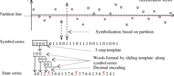
In the example shown in Figure 1, the window length and the sampling points of a raw acceleration data series are shown as small circles, which have dif- ferent values; the x-axis is time and the y-axis is accel- eration data. The partition line is the one with the mean value of the raw acceleration data series. Thus, the whole space is separated into two regions. The acceleration data that falls inside the upper region is symbolized by “1”; otherwise, it is “0”. The result of the symbolization is a binary coded symbol series that only contains “0” and “1”. In this example, a word length of 3 was used to cre-ate words, which means the first three symbols “1 0 0” are chosen as the first word, and the second to fourth
symbols “0 0 0” are chosen as the second word. By re-peating this procedure, 24 words can be created from the symbol series. Every binary coded word needs to be transformed into the decimal domain. Take the first word as an example. “1 0 0” can be transformed to
4
1 2 2 0 21 0 20
u
, which is called a “state”. A state series can be obtained after all the words are trans- formed from the binary domain to the decimal domain, which constitutes the values 0 - 7.
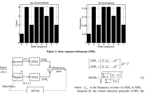
As shown in Figure 1, the occurrence number of cer- tain states in the state series varies. A bar graph used to plot the occurrence number of every state in a state series is called a “state sequence histogram” (SSH). The corre- sponding SSH for this example is plotted in Figure 2(a). Taking state “5” as an example, the corresponding count number is “3”, meaning that state “5” occurs three times in the state series (as marked in the state series of Figure 1). Also, the SSH can be normalized, which can be ac- complished by dividing the occurrence number of each state by the total number of states in the state series (Figure 2(b)).
3. Proposed Method
3.1. Procedure
In the research field of structural parameter identification, the time response of the system is usually compared with that of a parameterized model using a norm or some per- formance criterion to give us a measure of how well the model explains the system.
We will explain our methodology (Figure 3) using a physical system with input and output y. Let
i 1, ,
y t i T
, , ,
T ndenote the value of the actual system at the ith discrete time step. Suppose that a parameterized model able to capture the behavior of the physical system is developed and this model depends on a set of n
parameters, i.e., x x x1 2 xn R
ˆ. Given a can-
didate parameter value x and a guess X0 of the initial
state, y tˆ
i i1,,T
Acceleration series
1 0 0 0 1 0 1 1 0 0 1 1 1 0 1 1 1 0 0 1 1 0 1 0 0 1
, the value of the parameterized model, i.e., the identified system at the ith discrete time
y
1 0 0 0 0 0
0 0 1 Partition line
Symbol series
State series
Symbolization based on partition
Decimal encoding
Words formed by sliding template along symbol series
3-step template
x
[image:2.595.147.443.588.718.2]4 0 1 2 53 6 4 1 3 7 653 7 6 4 1 3 6 52 4 1
0 1 2 3 4 5 6 7 0
1 2 3 4
State sequen
C
ount
(a) Unnormali
ce zed
0 1 2 3 4 5 6 7
0 0.04 0.08 0.12 0.16
State sequen
F
requency
(b) Normaliz
[image:3.595.62.545.82.391.2]ce ed
Figure 2. State sequence histogram (SSH).
( )i
y t
( )i
u t
ˆ( , )i
y x t
System
Model
STSA
STSA Input
SSHa
AICSA Adjusting x
SSHb
E
0 1 1
0 1 1
, , ,
, 2 , , ,
Q
a a a a r
Q
b b b b
SSH d d d
Q
SSH d d d
Prediction error
[image:3.595.59.292.83.399.2]
iFigure 3. Procedure of AICSA combining STSA for identi- fication of structural parameters.
step, can be obtained. Hence, the problem of system identification boils down to finding a set of parameters that minimize the prediction error between the system output y t
ˆ , i ,
, which is the measured data, and the model output y x t which is calculated at each time instant
.
i
t
Usually, our interest lies in minimizing the predefined error norm of the time series outputs, e.g., the following mean square error (MSE) function,
2ˆ ,
i i
1
1 T i
f x y
T
t y x t (2)where ·
* n
represents the Euclidean norm of vectors. Formally, the optimization problem requires one to find a set of n parameters x R
( )
so that a certain quality criterion is satisfied, namely, that the error norm f is minimized. The function f( ) is called a fitness func- tion or objective function. Typically, an objective func- tion that reflects the goodness of the solution is chosen.
In our methodology, we introduce an index, the rela- tive state sequence histogram error (RSSHe), to measure the distance between SSHa and SSHb (SSHa and SSHb are
the system output and model output, respectively). The definition is:
2 1
0
2 1 0
i Q i i
b a
i
i Q i
a i
d d RSSHe
d
i
d
(3)
where a b/ is the frequency of state i in SSHa or SSHb.
Inspired by the clonal selection principle (CSP), the clonal selection algorithm (CSA) has been used to deal with optimization problems because of its search capa- bility is superior to those of classical optimization tech- niques [14].
Although CSA has great advantages over the genetic algorithm (GA), it is still difficult to use it to solve complex problems. To be able to solve complex pro- blems, in AICSA, three strategies, i.e., secondary re- sponse, adaptive mutation regulation and vaccination, are used to improve the CSA’s convergence speed and glo- bal optimum search. For detailed information about AICSA, please refer to [4,15].
3.2. Guideline for Parameter Selection
In STSA, the main parameters are the word length and window length, and they control the resolution of the whole representation space. For a window length T and word length r, two limiting cases of SSH are predefined as:
Case 1: All states in the SSH are distributed uniformly,
and the frequency of each state is 1
2r .
Case 2: Only one state in the SSH has the frequency of 1; the frequencies of the other states are 0.
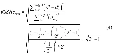
Suppose there are two different SSHs: SSHa and SSHb.
From Equation (3), when SSHa corresponds to limiting
case 1 and SSHb to limiting case 2, the maximum value
2 1 0max 1 2
0
2 2
2
1 1
(1 ) 2
2 2
1 * 2 2
i Q i i
b a
i
i Q i
a i r r r r r d d RSSHe d
12r 1
(4)
when SSHa and SSHb are the same, the minimum RSSHe
is 0. Then,
min, maxRSSHe RSSHe RSSHe 0, 2r1 (5)
Since the minimum changeable unit in SSH is 1
1
T r , the change in frequency of one state in SSH will ab- solutely be related to the change in frequencies of other states. Supposing that there are only two minimum unit differences between SSHa and SSHb, the minimum
distinguishable RSSHe is:
2 1 0dis 1 2
0 2 2 2 1 0 1 1 1 1
i Q i i b a i
i Q i a i
i Q i a i
d d
RSSHe
d
T r T r
d
2 1 0 2 1i Q i a i d T r
max dis RSSHe (6)when SSHa is limiting case 1, the maximum distin-
guishable will be:
( 1) max 2 1 r T r dis RSSHe min dis RSSHe (7)
when SSHa is limiting case 2, the minimum distin-
guishable will be:
mi dis
RSSHe n 2
1
T r
(8)
The resolution is:
1
2 2 , 1 1 r T r min max dis , dis
RSSHe RSSHe T r 2r (9)
Note that we also need to consider the number of the possible distributions of states in one SSH. If the number of states in SSH is and the minimum changeable unit
is 1
1
T r N
1
T r
2r
2 1 2
r
r
SSH T r
N C
, finding the total number of possible dis-
tributions SSH of SSH boils down to a classic com-
bination problem, which is “put identical balls in different boxes”. The combinatorial number is:
(10)
As we can see, longer window and word lengths are related to higher resolution, which means that the self and non-self spaces can be separated much more ac- curately. This is the key to obtaining accurate structural parameter identification.
So far, our discussion of the effect of the window length and word length has been based on a case in which only one story’s output (raw acceleration data) is used, but structures with multiple degrees of freedom (MDOF) may have more outputs than that. Supposing the outputs from N stories can be obtained, the boundary of the solution space is:
N
min, max
0, 2 1
N r
RSSHe RSSHe RSSHe
(11)
The resolution falls to:
min max dis dis 1 , 2 2 , 1 1 N N r RSSHe RSSHe
T r T r
2 12
r
r
(12)
Also, the total number of possible distributions in- creases to:
N N
SSH T r
N C
t t t
(13)
From Equations (11) to (13), it is evident that as more story outputs are obtained, the more accurate the identi- fication results will be.
4. Effects of Parameter Selection for SDOF
Model
4.1. Description of SDOF Model
For simplicity and generality, we used a single-story shear frame structure as a representative case to verify the effect of the parameters in STSA, and we modeled it as a single degree-of-freedom (SDOF) lumped mass sys- tem (Figure 4). As for the structure, its mass was 1000 kg, stiffness 1.000 MN/m, and natural frequency 5.032 Hz. The dynamic equation is [16]:
MX CX KX f t (13)
g
x
1, 1
k c
1
[image:4.595.69.289.84.188.2]m x1
30
where M, C, and K are respectively the mass matrix, damping matrix, and stiffness matrix. f t
is the force vector linked to the ground acceleration. X, X
, and X are respectively relative acceleration, velocity, and displacement response. The sampling frequency was 100 Hz. In the simulation, the input signal was Gaussian white noise. The root-mean-square error (RMSe) was used to verify the feasibility and performance of the identification results. RMSe is defined as
2 , real,
2 real, 1
c i i n
i i
k k
k
k
1
n i
RMSe
(14)where c i, and real,i are the candidate stiffness and
real stiffness of the ith story, respectively.
k
To test the noise immunity of our method, noise at levels of 5%, 10% or 20% was added to the raw accel- eration data.
4.2. Effect of Varying the Window Length and Word Length
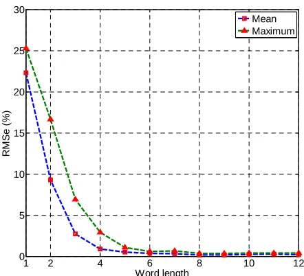
As stated before, the window length and word length are the control parameters in STSA. In the simulation, the mass distribution and damping parameters were assumed to be known and the stiffness of each story was set as the objective parameters that needed to be identified. In the first verification, the word length was varied from 1 to 12 and the window length was 3000. In the second verifica- tion, the word length was 9 and the window length was varied from 500 to 6000 at intervals of 500. Each test was run 10 times independently by choosing an initial value of AICSA randomly every time. The parameters of AICSA were the same as in [4,5].
Figures 5 and 6 indicate that the word length and window length greatly affected the performance of the methodology. Larger word and window lengths yielded better performance. The reason is that, as theoretically shown in Section 3.2 (Equations (4)-(10)), a longer word or window can symbolize the raw acceleration data much more accurately than a shorter one. As the word length and window length increase, much more dynamic infor- mation about the system is captured, the identified results become more accurate, and the maximum and mean
[image:5.595.312.533.82.283.2]RMSe decrease. In the simulation, a word length more than 9 and window length more than 3.0E+03 gave ac- ceptable results.
Table 1 (under the label “STSA”) lists the identifica- tion results of the SDOF structure using a word length of 9 and a window length of 3000 for different noise levels. For comparison, we estimated the parameters and RMSe
for an SDOF model using raw acceleration data as input, for a data length of 3000, i.e., the same as the window length in STSA; the results are listed under the label “RAW”.
1 2 4 6 8 10 12
0 5 10 15 20 25
Word length
RM
S
e
(
%
)
Mean Maximum
Figure 5. Effect of varying word length for a window length of 3000.
18
500 1000 2,000 3,000 4,000 5,000 6,000
2 4 6 8 10 12 14 16
Window length
RM
Se (
%
)
[image:5.595.313.532.322.513.2]Mean Maximum
[image:5.595.306.541.592.690.2]Figure 6. Effect of varying the window length for a word length of 9.
Table 1. Estimated parameters and RMSe for SDOF model using STSA (with word length 9 and window length 3000) or raw acceleration data as input.
Calculated value (MN/m) True
value
(MN/m) noise No noise 5% noise10% noise20%
k 1.000 1.000 1.000 1.000 1.000 STSA
RMSe 0.00% 0.00% 0.04% 0.04%
k 1.000 1.000 0.991 1.031 1.065 RAW
RMSe 0.00% 0.90% 3.12% 6.54%
As we can see, although AICSA using raw accelera- tion data gives good results for the noise-free case, its
trast, our method has good noise immunity; the identifi- cation results stay accurate as the noise level increases. Even for the high noise level of 20%, the RMSe of the results is only 0.04%.
5. Extension to MDOF Models
5.1. Description of MDOF Models
[image:6.595.311.536.112.458.2]Next, we tried to see if our methodology can be reliably used to identify the parameters of an MDOF system. Here, we choose three cases, a 3-DOF, 5-DOF (shown in
Figure 7 as an example) and 10-DOF structure, as exam- ples. These structures were modeled as multiple degree- of-freedom lumped mass systems. Table 2 summarizes the structural parameters. In these structures, the mass of each story was 1000 kg, and the stiffness of each story was 2.000 MN/m. The damping ratios of all MDOF structures were the same, i.e., 0.03 and 0.05 for the first and second modes, respectively.
5.2. RMSe for MDOF Models
In the input signal of the MDOF simulation, was Gaus- sian white noise, as was used in the SDOF simulation. The stiffness of each story was unknown and needed to be identified. The methodology of combining AICSA with STSA was compared with AICSA using raw accel- eration data. Window and word lengths were the same as before, and the full output of the structure was used.
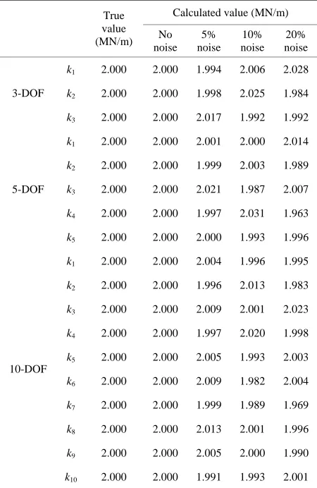
Table 3 lists the identified stiffness of each story of the 3, 5 and 10 DOF models. The estimated parameters for the 3, 5 and 10 DOF models using AICSA using raw acceleration are not listed for lack of space, but Table 4
summarizes the RMSe of the identification results of the 3, 5 and 10 DOF models using AICSA combining with STSA as well as AICSA using raw acceleration data.
4 m
3 m
2 m
1 m
4, 4 k c
3, 3 k c
2, 2 k c
1, 1 k c
3 x
2 x
1 x
g
x
3rdstory
2ndstory
1ststory
4thstory
5thstory m5
5, 5 k c
4 x
5 x
[image:6.595.312.537.498.640.2]
[image:6.595.97.245.524.639.2]Figure 7. 5-DOF shear frame structure.
Table 2. Parameters of MDOF models.
DOF 1 2 3 4 5
Mass (kg) 1000 1000 1000 1000 1000
Stiffness (MN/m) 2.000 2.000 2.000 2.000 2.000
Table 3. Estimated parameters for 3, 5 and 10 DOF models with a word length of 9 and window length of 3000.
Calculated value (MN/m) True
value
(MN/m) noise No noise 5% noise10% noise20%
k1 2.000 2.000 1.994 2.006 2.028 k2 2.000 2.000 1.998 2.025 1.984 3-DOF
k3 2.000 2.000 2.017 1.992 1.992 k1 2.000 2.000 2.001 2.000 2.014 k2 2.000 2.000 1.999 2.003 1.989 k3 2.000 2.000 2.021 1.987 2.007 k4 2.000 2.000 1.997 2.031 1.963 5-DOF
k5 2.000 2.000 2.000 1.993 1.996 k1 2.000 2.000 2.004 1.996 1.995 k2 2.000 2.000 1.996 2.013 1.983 k3 2.000 2.000 2.009 2.001 2.023 k4 2.000 2.000 1.997 2.020 1.998 k5 2.000 2.000 2.005 1.993 2.003 k6 2.000 2.000 2.009 1.982 2.004 k7 2.000 2.000 1.999 1.989 1.969 k8 2.000 2.000 2.013 2.001 1.996 k9 2.000 2.000 2.005 2.000 1.990 10-DOF
k10 2.000 2.000 1.991 1.993 2.001
Table 4. RMSe for 3, 5 and 10 DOF models using STSA or raw acceleration as input.
RMSe
No noise
5% noise
10% noise
20% noise
3-DOF 0.00% 0.91% 1.35% 1.66%
5-DOF 0.00% 1.08% 1.74% 2.08% SATA
10-DOF 0.02% 1.11% 1.68% 2.21%
3-DOF 0.00 % 3.11% 5.38% 8.39 %
5-DOF 0.00% 1.47% 3.99% 5.67% RAW
10-DOF 0.07% 4.26% 5.84% 10.01%
[image:6.595.59.286.679.734.2]1-DOF 3-DOF
5-DOF 10-DOF Noise level 20%
Noise level 10% Noise level 5%
Noise level 0 0
0.5 1 1.5 2 2.5
RM
S
e
(
%
[image:7.595.61.288.85.244.2])
Figure 8. RMSe for 1, 3, 5 and 10 DOF models.
solution space of the identification problem becomes much more complex as the DOF go up.
Moreover, AICSA combining STSA outperformed AICSA using raw acceleration data (results under the “RAW” label in Table 1 and 4) on the MDOF models. Furthermore, it provided much better estimates when the output data was contaminated with noise. These results clearly show that our methodology has excellent noise immunity.
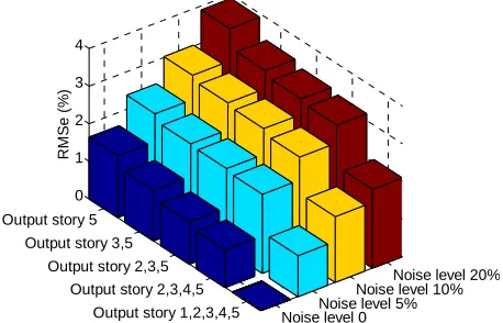
5.3. Estimation Using Partial Outputs
The simulations results of the MDOF structures are based on the full output of the structural acceleration data. For an SDOF structure, only one output can be used, but for MDOF structures, it may be the case that not all out- puts are available. Therefore, to verify the methodology on only partial output, a 5-DOF structure was simulated and data from some of its stories (randomly chosen) were used. The simulated output data was noise-free, with 5% noise, 10% noise, or 20% noise. The window length was 3000, and the word length was 9.
The results in Figure 9 illustrate that even using par- tial data, the proposed method gets acceptable results. Note that for a certain noise level, the RMSe of the iden- tification results increase as the number of outputs de- creases. Moreover, Equations (11)-(13) can be numeri- cally proved to be right as t more outputs are obtained.
6. Conclusion
We conducted a feasibility study of a parameter identifi- cation method based on symbolic time series analysis (STSA) and adaptive immune clonal selection algorithm (AICSA). Harmful noise in the raw acceleration data was alleviated by employing STSA. The effect of varying the parameters of word length and window length in STSA was evaluated theoretically and verified numerically. A comparison with AICSA using raw acceleration data
Noise level 0Noise level 5%
Noise level 10%Noise level 20% Output story 5
Output story 3,5 Output story 2,3,5
Output story 2,3,4,5 Output story 1,2,3,4,5 0
1 2 3 4
RM
S
e
(
%
)
Figure 9. Comparison of RMSe due to partial output.
revealed that our methodology provided better estimates of structural parameters when the data was contaminated by noise. The results show that with the proper parame- ters, our methodology is a reliable and effective method for structural parameter identification.
7. Acknowledgements
This work was supported in part by a Grant-in-Aid No. 22310103 (PI: A. Mita) and Grant-in-Aid to the Global Center of Excellence Program for the “Center for Educa- tion and Research of Symbiotic, Safe and Secure System Design” from the Ministry of Education, Culture, Sport, Science and Technology of Japan.
REFERENCES
[1] R. I. Levin and N. A. J. Lieven, “Dynamic Finite Element Model Updating Using Simulated Annealing and Genetic Algorithms,” Mechanical Systems and Signal Processing, Vol. 12, No. 1, 1998, pp. 91-120.
doi:10.1006/mssp.1996.0136
[2] K. Cunha and V. V. Smith, “A Determination of the Solar Photospheric Boron Abundance,” Astrophysical Journal, Vol. 512, No. 2, 1999, pp. 1006-1013.
doi:10.1086/306796
[3] S. T. Xue, H. S. Tang and J. Zhou, “Identification of Structural Systems Using Particle Swarm Optimization,” Journal of Asian Architecture and Building Engineering, Vol. 8, No. 2, 2009, pp. 517-524.
doi:10.3130/jaabe.8.517
[4] R. Li and A. Mita, “Structural Damage Identification Using Adaptive Immune Clonal Selection Algorithm and Acceleration Data,” SPIE Smart Structures, Vol. 7981, 2011, Article ID: 79815A.
[5] R. Li and A. Mita, “Hybrid Immune Algorithm for Structural Health Monitoring Using Acceleration Data,” 8th International Workshop on Structural Health Moni- toring, Stanford, September 2011, pp. 1095-1102. [6] R. K. Ursem and P. Vadstrup, “Parameter Identification
[image:7.595.309.538.89.236.2]putation, Vol. 2, 2003, pp. 790-796.
[7] H. S. Tang, S. T. Xue and C. X. Fan, “Differential Evolution Strategy for Structural Parameter Identifi- cation,” Computers & Structures, Vol. 86, No. 21-22, 2008, pp. 2004-2012.
doi:10.1016/j.compstruc.2008.05.001
[8] A. Ray, “Symbolic Dynamic Analysis of Complex Sys- tems for Anomaly Detection,” Signal Processing, Vol. 84, No. 7, 2004, pp. 1115-1130.
doi:10.1016/j.sigpro.2004.03.011
[9] S. Chin, A. Ray and V. Rajagopalan, “Symbolic Time Series Analysis for Anomaly Detection: A Comparative Evaluation,” Signal Processing, Vol. 85, No. 9, 2005, pp. 1859-1868.doi:10.1016/j.sigpro.2005.03.014
[10] A. Khatkhate, A. Ray, S. Chin, V. Rajagopalan and E. Keller, “Detection of Fatigue Crack Anomaly: A Sym- bolic Dynamic Approach,” Proceedings of American Con- trol Conference, Boston, June-July 2004, pp. 3741-3746. [11] D. Tolani, M. Yasar, A. Ray and V. Yang, “Anomaly
Detection in Aircraft Gas Turbine Engines,” AIAA Jour- nal of Aerospace Computing Information, and Com- munication, Vol. 3, No. 2, 2006, pp. 44-51.
doi:10.2514/1.15768
[12] S. Bhatnagar, V. Rajagopalan and A. Ray, “Incipient Fault Detection in Mechanical Power Transmission Sys- tems,” Proceedings of American Control Conference, Portland, 8-10 June 2005, pp. 472-477.
doi:10.1109/ACC.2005.1469980
[13] R. Samsi, V. Rajagopalan, J. Mayer and A. Ray, “Early Detection of Voltage Imbalances in Induction Machines,” Proceedings of American Control Conference, Portland, 8-10 June 2005, pp. 478-483.
doi:10.1109/ACC.2005.1469981
[14] X. Wang, X. Z. Gao and S. J. Ovaska, “Artificial Immune Optimization Methods and Applications—A Survey,” IEEE International Conference on Systems, Man and Cybernetics, Vol. 4, 2004, pp. 3415-3420.
[15] L. Zhang, X. R. Meng, W. J. Wu and H. Zhou, “Network Fault Feature Selection Based on Adaptive Immune Clonal Selection Algorithm,” International Joint Con- ference on Computational Sciences and Optimization, Sanya, 24-26 April 2009, pp. 969-713.
doi:10.1109/CSO.2009.342