An adaptive orthogonal search algorithm for model subset selection and non-linear system identification

promoting access to White Rose research papers

Universities of Leeds, Sheffield and York

http://eprints.whiterose.ac.uk/

This is an author produced version of a paper published in International Journal

of Control.

White Rose Research Online URL for this paper:

http://eprints.whiterose.ac.uk/8555/

Published paper

Wei, H.L and Billings, S.A (2008)

An adaptive orthogonal search algorithm for

model subset selection and non-linear system identification.

International Journal

of Control, 81 (5). pp. 714-724.

A prepublication draft of the paper published in

International Journal of Control, Vol. 81, No. 5, pp.714-724, 2008.

An Adaptive Orthogonal Search Algorithm for Model Subset

Selection and Nonlinear System Identification

S. A. Billings and H. L. Wei

Department of Automatic Control and Systems Engineering, University of Sheffield Mappin Street, Sheffield, S1 3JD, UK

[email protected], [email protected]

Abstract: A new adaptive orthogonal search (AOS) algorithm is proposed for model subset selection

and nonlinear system identification. Model structure detection is a key step in any system

identification problem. This consists of selecting significant model terms from a redundant dictionary

of candidate model terms, and determining the model complexity (model length or model size). The

final objective is to produce a parsimonious model that can well capture the inherent dynamics of the

underlying system. In the new AOS algorithm, a modified generalized cross-validation criterion,

called the adjustable prediction error sum of squares (APRESS), is introduced and incorporated into a

forward orthogonal search procedure. The main advantage of the new AOS algorithm is that the

mechanism is simple and the implementation is direct and easy, and more importantly it can produce

efficient model subsets for most nonlinear identification problems.

An Adaptive Orthogonal Search Algorithm for Model Subset

Selection and Nonlinear System Identification

S. A. Billings and H. L. Wei

Department of Automatic Control and Systems Engineering, University of Sheffield Mappin Street, Sheffield, S1 3JD, UK

[email protected], [email protected]

Abstract: A new adaptive orthogonal search (AOS) algorithm is proposed for model subset selection

and nonlinear system identification. Model structure detection is a key step in any system

identification problem. This consists of selecting significant model terms from a redundant dictionary

of candidate model terms, and determining the model complexity (model length or model size). The

final objective is to produce a parsimonious model that can well capture the inherent dynamics of the

underlying system. In the new AOS algorithm, a modified generalized cross-validation criterion,

called the adjustable prediction error sum of squares (APRESS), is introduced and incorporated into a

forward orthogonal search procedure. The main advantage of the new AOS algorithm is that the

mechanism is simple and the implementation is direct and easy, and more importantly it can produce

efficient model subsets for most nonlinear identification problems.

Keywords: cross-validation, information criterion, leave-one-out, model structure detection, prediction error sum of squares.

1. Introduction

A wide class of input-output nonlinear dynamical systems can be represented by the NARX

(Nonlinear AutoRegressive with eXogenous inputs) model of the form

y(t)= f(y(t−1),_L,y(t−n_y),u(t−1),_L,u(t−n_u))+e(t) (1)

where the nonlinear mapping is often unknown and needs to be identified from given observational

data of the input and the output ; and are the maximum input and output lags; is

the model prediction error, which can often be treated as an independent zero mean noise sequence

providing that the function gives a sufficient description of the system. The nonlinear

f

) (t

u y(t)

n

mapping can be constructed using a variety of local or global basis functions including polynomials,

kernel functions, splines, radial basis functions, neural networks and wavelets. A NARX model

constructed using basis function expansions can be expressed using a linear-in-the-parameters form

f ) ( ) ( ) ( 1 t e t t y M m m m + =

∑

θ (2)

whereφ_m(t)=φ_m(ϕ(t)) are model terms generated in some way from the regression vector ϕ(t)

, ,

), 1 (

[ − _L

= y t y(t−n_y),u(t−1),_L, T u

n t

u( − )] θ_m are unknown parameters, and M is the number

of total potential model terms involved. One of the most popular representations is the polynomial

model, which takes the form below

∑

∑ ∑

= = + = + + + = d i d i i i i i i d i i

i x t f x t x t

f t y 1 1 1 0

1 2 1

2 1 2 1 1 1

1( ( )) ( ( ), ( ))

) ( θ ) ( )) ( , ), ( ), ( ( 1 1 1 2 1 2 1 1 t e t x t x t x f _i d i i i i i i i d i + +

∑

∑

L L (3)

where

m i i i12L

θ

∏

i x t x t x t x t

f k m m m 1 ) ( )) ( , ), ( ), ( ( 2 1 2 1 2

1 L L θ L

1

≤

m

≤

l

(5) ⎪⎩ ⎪ ⎨ ⎧ ≤ ≤ + − − ≤ ≤ − = d k n n k t u n k k t y t x y y y k 1 )) ( ( 1 ) ( ) (

The degree of a multivariate polynomial is defined as the highest order among the terms, for example,

the degree of the polynomial is determined by the term

and thus 2+1+2=5. Similarly, a NARX model with a nonlinear degree

_l

order of each term in the model is not higher than

_l

2 3 2 2 1 3 3 2 2 4 1 1 3 2

1, , )

(x x x a x a x x a x x x

h = + +

2 3 2 2 1x x

x

_l

=

The initial linear-in-the-parameters model (2) may involve a large number of candidate model

terms whatever basis functions are employed to approximate the unknown nonlinear mapping ,

especially when the maximum lags and are large. Experience shows that in most cases only a

small number of significant model terms are necessary in the final model to represent given

observational data. Most candidate model terms are either redundant or make very little contribution

f

u

to the system output and can therefore be removed from the model. An efficient model structure

determination approach has been developed based on the orthogonal forward regression (OFR)

algorithm and the error reduction ratio (ERR) criterion (an index indicating the significance of each

model term), which was originally introduced to determine which terms should be included in a

model (Billings et al. 1989, Chen et al. 1989). This approach has been extensively studied and widely

applied in nonlinear system identification (Billings and Jones 1992, Chen et al. 1991, 2004a, 2004b,

Zhu and Billings 1996, Hong et al. 2003, 2004, Wei et al. 2004).

The standard OFR-ERR algorithm provides a powerful tool to effectively select significant model

terms step by step, one at a time, by orthogonalizing the associated regressors and maximizing the

ERR criterion, in a forward stepwise way. The standard OFR-ERR algorithm, however, does not

provide information on how many significant model terms should be included in the final model, and

the search procedure is often terminated when the ERR value arrives at a threshold that is heuristically

or empirically chosen in advance. An additional separate procedure is therefore often needed to aid

the determination of the optimal or suboptimal number of significant model terms. To ameliorate the

effectiveness of the OFR-ERR algorithm, Hong et al. (2003) and Chen et al. (2004a, 2004b) have

introduced a cross-validation type criterion, which was referred to as the leave-one-out (LOO) test

score, also called the predicted residual sums of squares (PRESS), and have incorporated the criterion

into the OFR algorithm, to facilitate the determination of the optimal number of model terms.

Motivated by the successful applications of the OFR-ERR algorithm for model structure detection

and inspired by the affirmative potential of cross-validation for model selection, this study aims to

develop a new adaptive orthogonal search (AOS) scheme that can be used to select significant model

terms, to capture the inherent dynamics of the underlying system, and to determine the optimal

number of model terms, to arrive at a good balance for the bias-variance trade-off. In the new AOS

algorithm, a modified LOO type cross-validation criterion, called the adjustable prediction error sum

of squares (APRESS), is introduced and integrated into a forward orthogonal search algorithm. The

new AOS scheme has been developed to achieve the following objectives: i) to detect significant

output; ii) to determine the optimal number of model terms to arrive at a good balance between the

bias-variance trade-off and, iii) to estimate the unknown model parameters.

The present study has a relationship with but does not focuses on the model variable and model

order (or lag) selection problem (Tjostheim and Auestad 1994, Vieu 1995, Tschernig and Yang 2000,

Gonzalez-Manteiga et al. 2002, Huang and Yang 2004). On the contrary, this study treats the model

variable and model lag selection problem as a special case. However, if the model variable and model

lag selection problem for a given system can be efficiently solved at the first stage, the model

structure detection problem, which is the main focus here, can then be significantly simplified.

This paper is organized as follows. In Section 2, the basic idea of adaptive orthogonal search

algorithm for model selection is described. In Section 3, the performance of the new AOS algorithm is

tested by studying two illustrative examples. The work is concluded in Section 4.

2. The adaptive orthogonal search algorithm

2.1 The forward orthogonal search procedure

Consider the term selection problem for the linear-in-the-parameters model (2).

Let _{[y(1), ,y(N)]}Tbe a vector of measured outputs at N time instants, and

L =

y φ_m =[φ_m(1),_L,

be a vector formed by the mth candidate model term, where m=1,2, …, M. Let

be a dictionary composed of the M candidate bases. From the viewpoint of practical

modelling and identification, the finite dimensional set D is often redundant. The model term

selection problem is equivalent to finding a full dimensional subset

T m(N)] φ

} , , {φ1L φM =

D

} , , { 1 n n= α L α

D of

n ( ) bases, from the libraryD, where

} , , {

1 in

i φ

φ _L

=

M n≤

k i k φ

α = , ik∈{1,2,L,M} and k=1,2, …, n, so that ycan

be satisfactorily approximated using a linear combination of α₁,α₂,_L,α_n as below

e

α α

y=θ1 1+L+θn n+ (6)

or in a compact matrix form

e Aθ

where the matrix is assumed to be of full column rank, is a parameter

vector, and is the approximation error. ]

, , [α1 αn

A= _L T

n]

, , [θ_1L θ

=

θ

e

Following Billings et al. (1989) and Chen et al. (1989), a squared correlation coefficient will be

used to measure the dependency between two associated random vectors. The squared correlation

coefficient between two vectors x and y of size N is defined as

∑

∑

∑

2 _{( )}

) )( ( ) ( ) , ( y y x x y x y

x (8)

The model structure selection procedure starts from equation (2). Let r₀ =y, and

)} , ( { max arg 1

1= _≤j≤M C y φj

l (9)

where the functionC(⋅,⋅)is the correlation coefficient defined by (8). The first significant basis can

thus be selected as , and the first associated orthogonal basis can be chosen as . The

model residual, related to the first step search, is given as

1

1 φl

α =

1

1 φl

q = 1 1 1 1 0 1 q q q q y r r _T T −

= (10)

In general, the mth significant model term can be chosen as follows. Assume that at the (m-1)th

step, a subset , consisting of (m-1) significant bases, , has been determined, and

the (m-1) selected bases have been transformed into a new group of orthogonal bases

via some orthogonal transformation. Let

1

− m

D α1,α2,L,αm−1

1 2

1,q , ,qm−

q _L

∑

q (11)

)} , ( { max

arg ( )

1 1 , m j m k j m C k q y − ≤ ≤ ≠ = l

l (12)

where , and is the residual vector obtained in the (m-1)th step. The mth significant

basis can then be chosen as and the mth associated orthogonal basis can be chosen as

. The residual vector at the mth step is given by

1

−

−

∈ _m

j D D

φ r_m−1

m m φl

α =

) (m m qlm

m m T m m T m

m _{q q} q

q y r

r = ₋₁− (13)

Subsequent significant bases can be selected in the same way step by step. From (13), the vectors

and are orthogonal, thus

m

r qm

m T m m T m m q q q y r

r 2 2

1

2 _{|| ||} ( )

||

|| = ₋ − (14)

By respectively summing (13) and (14) for m from 1 to n, yields

n n m m m T m m T r q q q q y y

∑

∑

m Tm m m T n 1 2 2

2 _{|| ||} ( )

|| || q q q y y

r (16)

The model residual will be used to form a criterion for model selection, and the search procedure

will be terminated when the norm satisfies some specified conditions.

n

r

2

|| ||r_n

2.2 Parameter estimation

It is easy to verify that the relationship between the selected original bases , and the

associated orthogonal bases , is given by

n α α α₁, ₂,_L,

n

q q q1, 2,L,

n n n Q R

A = (17)

where , is an matrix with orthogonal columns , and is an

unit upper triangular matrix whose entries ]

, , [ 1 n

n α α

A = _L Qn N×n q1,q2,L,qn Rn

n

n× u_ij(1≤i≤ j≤n) are calculated during the

orthogonalization procedure. The unknown parameter vector, denoted by , for the

model with respect to the original bases (similar to (6)), can be calculated from the triangular equation

with , where for k=1,2, …, n.

T n n =[θ1,θ2,L,θ ]

θ

n n nθ g

R = T

n n =[g1,g2,L,g ]

g ( )/( T _k)

k k T k

g = y q q q

2.3 M

odel length determination

The determination of model size is critical in dynamical modelling. Neither an over-fitting nor an

under-fitting model is desirable in practical identification. In practice, however, the true model length

is generally unknown and needs to be estimated during model identification. Model selection criteria

model performs on future (never used) data sets. One general routine for model selection, which tries

to avoid or reduce any possible bias introduced by relying on any particular test data sets, is cross

validation (Stone 1974, Stoica et al. 1986). Cross-validation has a number of variations, two

commonly used variants of which are the leave-one-out (LOO), also called predicted sum of squares

(PRESS) (Allen 1974), and generalised cross-validation (GCV) (Craven and Wahba 1979, Golub et

al. 1979). Generalised cross-validation, due to its convenience of use and effectiveness for avoiding

overfitting, has been widely accepted.

In this study, an adjustable prediction error sum of squares (APRESS), formed using the PRESS

statistic, is employed to solve the model length determination problem. Consider the

linear-in-the-parameters model that is fitted using N available data point pairs and consists of n model terms given

by (6) and (7). The PRESS statistic (Allen 1974) is defined as

∑

∑

n i _N i

y i y N n 1 2 ) ( 1 2 )

( _()] 1 _{[ ()]}

ˆ ) ( [ 1 ]

PRESS[ ε (18)

where is the one-step-ahead prediction from a model of n model terms, fitted using a data set

consisting of N-1 observational data point pairs, which are obtained by leaving the ith point pair out,

are the PRESS predicted residuals evaluated at the ith point. Let )

( ˆ( ) _i

y i n−

) (

) ( i _i n−

ε ε(i)be the normally defined

residuals of a model fitted using the total N data points, it can be shown (Myers 1990) that the

relationship between ( i)(_i) and

n−

ε ε(i) is

2

1 1 ( , )

) ( 1 ] PRESS[

∑

i h i i

i N

n ε (19)

where , and and

A

can be calculated by fitting only one model using the total N data points, but N “leave-one-out”

matrices are still required. However, for the case , which is an often encountered scenario and

which will be considered in the present study, the calculation work of (19) can be significantly

reduced further (Miller 1990)

i T T i i i

h_{(, )=}α ₍A A₎−1α

i α n N >> ] MSE[ / 1 1 ] PRESS[ 2 n N n n ⎟ ⎠ ⎞ ⎜ ⎝ ⎛ −

where , indicating the mean-squared-errors (residuals) calculated

from the associated n-term model, is the one-step-ahead prediction sequence from the

identified model of n model terms. Statistic (20) consists of two parts: the mean-squared-error of the

fit to the data, and the penalty, , increasing model complexity (number of model terms).

Clearly this is one version of commonly used generalized cross-validation.

∑

= N

i y i y i

N n 1 2 )] ( ˆ ) ( [ ) / 1 ( ] MSE[ N i i yˆ( )} ₁ { ₌ 2 )] / ( 1 [ − n N

Experience has shown that the criterion given by (20) is prone to produce an over-fitted model

(Friedman and Silverman 1989, Barron and Xiao 1991). To avoid the tendency that the role of the

penalty is mitigated by a large N, and thus to avoid overfitting, the present study, following Friedman

and Silverman (1989) and Friedman (1991), suggests using an adjustable PRESS statistic (APRESS)

defined as below

] MSE[ / ) , ( 1 1 ] MSE[ ] [ ] APRESS[ ] [ 2 n N n C n n p n n J _⎟⎟ ⎠ ⎞ ⎜⎜ ⎝ ⎛ − = = =

α (21)

where C(n,α)=1−nα/N , with α ≥1 , is the complexity cost function, and

is the penalty function. The statistic is ready to incorporate into the

forward orthogonal search procedure. Indeed, by using the relationship , the value

for J[n] can easily and directly be calculated from .

2 )] / ) , ( [ 1 /[ 1 ]

[n C n N

p = − α

N n] || _n|| / MSE[ _{= r} 2

2

|| ||r_n

Notice that the PRESS statistic defined by (20) is different from that used in Hong et al. (2003)

and Chen et al. (2004a, 2004b), where at each search step the PRESS statistic was calculated using

the definition (19) and the orthogonal factorization property (17), and the criterion was formed in

terms of the model residual and the orthogonal bases as: PRESS[n]=

and

n

r q₁,q₂,L,q_n

∑

t rn t n t

N

1

2 2_{()/ ()]}

[ ) / 1

( β () 1 [ ()/|| ||2]

1 2

i n

i i n t = −

∑

β 2 2

1( ) i( )/|| n|| n t −q t q

=β ₋ , withβ₁(t)=1.

In the model selection procedure, regularised by the APRESS statistic here, any computation load on

the vector and matrix calculations required by the original PRESS statistic (19) is avoided, and the

3. Simulation studies

This section investigates the efficiency and performance of the new AOS algorithm, by applying

this algorithm to two examples. The first example is for a simulated data set, while the second

example is for a real data set.

Notice that in many cases the noise signal in Eq. (1) may be a correlated or coloured noise

sequence and this is likely to be the case for most real data sets of dynamical nonlinear systems. In

this case the associated resulting models may fail to give a sufficient description due to the bias in the

parameter estimates. Practical identification experience shows that the bias on the parameter estimates

can be virtually eliminated by including the noise signals )

(t e

) ( , ), 1

(t e t n_e

e − _L − in the model. Readers

are referred to Billings et al. (1989), Billings and Chen (1998), and Billings and Wei (2005) for

detailed discussions.

In the simulation studies given below, a noise model of a linear polynomial form was used to

reduce the bias on the initial estimated parameters, and noise terms were then omitted from the model

when the models were used for prediction.

3.1 A simulated data set

Consider a nonlinear system described by the model below

) 2 ( ) 1 ( 5 . 0 | ) 1 ( | ) 1 ( )

(_{t =−u t− y t− + u}3 _{t− +u t−}

y +ξ(t) (22)

where the input u(t) was assumed to be bounded in [-1, 1], and ξ(t)was a noise determined by

) 2 ( 6 . 0 ) 1 ( 3 . 0 ) ( )

(t =wt + wt− + wt−

ξ (23)

with a Gaussian white noise of zero mean and a standard variation . The model was

simulated by setting the input signal u(t) as a random sequence uniformly distributed in [-1,1] and

1500 input-output data point were collected. The first 500 points were discarded and the remaining

1000 data points were used for model estimation and model performance test. The 1000 data points

were partitioned into two parts: the first 400 points were used for model estimation and the remaining

600 points were used for model validation. )

(t

w 2 ₌0.01

The regression vector (the ‘input’ vector), ϕ(t) in the representation (2), was chosen to be

T

t x t x t x t x

t) [ ( ), ( ), ( ), ( )] ( = _{1 2 3 4}

ϕ =[y(t−1),y(t−2),u(t−1),u(t−2)]T, and the initial model was chosen

to be a polynomial form given by (3), with the nonlinear degree

_l

=

involves a total of 84 candidate model terms. The AOS algorithm was used to select and rank

significant model terms. By setting the adjustable parameter α to beα=0, 1, …, 8, the APRESS

statistic, versus different model length, over the estimation (training) data set, were calculated and

these are shown in Figure 1.

The most interesting thing that can be seen in Figure 1 is that there is an apparent turning point at

horizon 4, for different values of the adjustable parameterα. Does this distinct turning point suggest

the right model size? To answer this question, the performance of the eight models, corresponding to

α=1, 2, …, 8, was studied and compared further by inspecting the predicative capability of these

models, and the associated results are shown in Table 1.

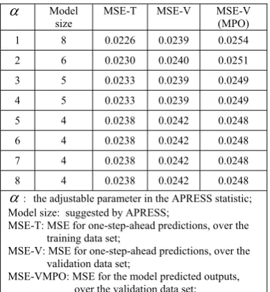
From Table 1, the PRESS statistic (the conventional generalized cross-validation) suggests

choosing eight model terms, while the APRESS statistic, with the adjustable parameterα ≥5 ,

suggests choosing four model terms. Compared with other models, the 4-term model is a good choice,

because this model, with a fewer number of model terms, possesses a slightly better predictive

capability. Clearly, for the simulated data set, the APRESS statistics is superior to the conventional

PRESS statistic.

To show that the 4-term model is valid and sufficient to describe the original system, a model

validity test approach, based on high order statistic analysis (Billings and Van 1986), was applied to

the model given below

) 1 ( 49048 . 0 )

(t =− u t−

y +1.0002u(t−2)₋0.41405_y2(_t−1)_u(_t−1) _+0.46134u3_{(t−1) +e(t) (24)}

Let )ε(t be the model residual (the one-step-ahead prediction). If the model structure and parameter

values are correct,ε(t)will be unpredictable from all linear and nonlinear combinations of past inputs

and outputs. For nonlinear SISO systems, this can be tested by computing the following correlation

Figure 1. The APRESS statistic versus the model size, over the training data set. The lines from the bottom to the top corresponding toα=0,1, …, 8. The bottom line with circles, corresponding toα=0, indicates the mean-squared-errors (MSE).

Table 1. A compassion of the performance of different models for the system described in Example 1 .

α Model size

MSE-T MSE-V MSE-V (MPO) 1 8 0.0226 0.0239 0.0254

2 6 0.0230 0.0240 0.0251 3 5 0.0233 0.0239 0.0249

4 5 0.0233 0.0239 0.0249

5 4 0.0238 0.0242 0.0248

6 4 0.0238 0.0242 0.0248 7 4 0.0238 0.0242 0.0248

8 4 0.0238 0.0242 0.0248

α: the adjustable parameter in the APRESS statistic; Model size: suggested by APRESS;

MSE-T: MSE for one-step-ahead predictions, over the training data set;

MSE-V: MSE for one-step-ahead predictions, over the validation data set;

⎪ ⎪ ⎪ ⎩ ⎪ ⎪ ⎪ ⎨ ⎧ ≥ = + + = ∀ = + = ∀ = + = ∀ = + = ∀ = + = 0 , 0 )} 1 ( ) ( ) ( { E ) ( , 0 )} ( ) ( { E ) ( , 0 )} ( ) ( { E ) ( , 0 )} ( ) ( { E ) ( , ) ( )} ( ) ( { E ) ( ) ( 2 2 2 2 2 2 τ τ ε ε τ γ τ τ ε τ γ τ τ ε τ γ τ τ ε τ γ τ τ δ τ ε ε τ γ ε ε ε ε ε εε t t u t t t u t t u t t u t t u u u u (25)

where

_u

(

_t

)

₌

_u

(

_t

)

₋

_u

(

_t

)

is that for a model to be statistically valid, there should be no predictable terms in the residuals. In

practice, however, only a finite data length will be available. This implies that confidence bands

should be used to reveal if the correlation between variables is significant or not. For large N (the data

length), the 95% confidence bands are approximately ] ( [ E ) ( 2

2 _{t u t}

u − N / 96 . 1

± and any significant correlation will

be indicated by one or more points of the function lying outside these bands.

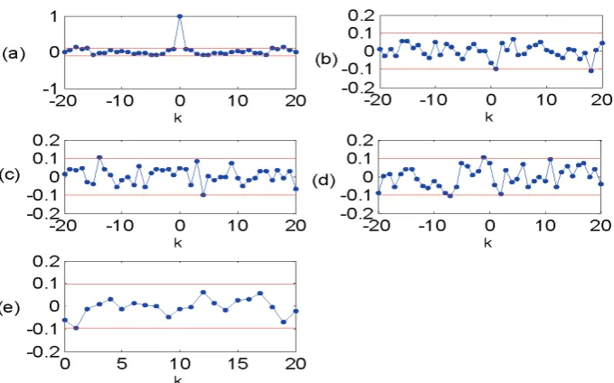
The five correlation functions were calculated using model (24), over the test data set consisting

of N=400 data points, and the results are shown in Figure 2, where the two horizontal lines with

amplitudes of about ±1.96/ N , in each graph, indicate the 95% confidence interval of the

associated correlation function. Clearly the correlation validity tests are all satisfied for the 4-term

model.

3.2 A real data set

—fruit fly modelling

This data set contains 1000 experimental data points for a wild type fly, called Drosophila. The

system input was the response of the photoreceptors, and the output was the response of the large

monopolar cells. The relationship between the input and the output in the fruit fly experiment is

complex, because in addition to the response from the photoreceptors, several other factors may also

affect the output response of the large monopolar cells. The objective here was to find a model that

reflects, as closely as possible, the relationship between the response of the photoreceptors (the input)

and the response of the large monopolar cells (the output), to facilitate the analysis and understanding

of the associate behaviour of this kind of insect.

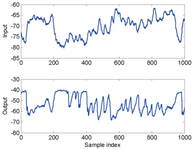
The 1000 input-output data points, which are shown in Figure 3, were partitioned into two parts:

the first 750 points were used for model estimation, and the remaining 250 points were used for model

performance test.

A nonlinear finite impulse response (NFIR) model was employed to describe the input-output

relationship of the fruit fly data. NFIR is a special case of the NARX model (3), where the regression

) (t

ϕ vector contains no lagged output y(t-k), with k≥1. The regression vector ϕ(t)for the fruit fly

data was chosen to be ϕ(t)=[x₁(t),x₂(t),_L,x₁₅(t)]T =[u(t−1),u(t−2),_L, u(t−15)]T , and the

nonlinear degree was chosen to be

_l

=

∑∑

∑

= = =

− − +

− +

= 15

1 15

, 15

1

0 ( ) ( ) ( )

) (

i j i i j i i

j t u i t u i

t u t

y θ θ θ +e(t) (26)

The initial model involves a total of 136 candidate model terms. By setting the adjustable parameter

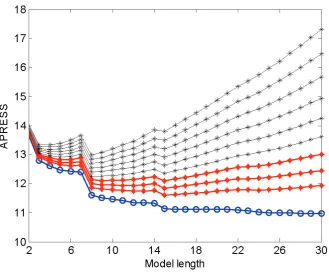
α to beα=0, 1.0, 1.5, 2.0, 2.5, …, 5, the APRESS statistic, versus different model length, over the

estimation (training) data set, were calculated and these are shown in Figure 4, where it can be seen

that there are two apparent turning points at horizon 8 and 15, for different values of the adjustable

parameterα. The PRESS statistic suggests choosing 15 model terms, while the APRESS statistic,

with the adjustable parameterα≥2.5, suggests choosing eight model terms. The performance of the

two models, consisting of 15 and 8 model terms, is shown in Table 2 and Figure 5. It is clear from

Table 2 and Figure 5 that the performance of the two models is comparable while the model of 8

model terms is slightly better on the validation data set. Again, for the fruit fly data, the APRESS

statistics provides more informative information, compared with the conventional PRESS statistic, for

model subset selection.

4. Conclusion

An efficient fast adaptive orthogonal search (AOS) algorithm has been developed for subset

selection and nonlinear system identification. In the new AOS algorithm, a new indicator, the

adjustable prediction error sum of squares (APRESS), has been introduced. The new AOS algorithm

was developed by incorporating the APRESS statistic into an efficient forward orthogonal search

algorithm. The combined AOS algorithm is multifunctional and can be used for model term selection,

model size determination, and parameter estimation. The new AOS scheme thus provides an efficient

Figure 3. The input and output data for the fruit fly system.

Figure 4. The APRESS statistic versus the model size, over the training data set, for the fruit fly modelling problem. The lines from the bottom to the top corresponding toα=0, 1.0, 1.5, 2.0, 2.5, …, 5. The bottom line with circles, corresponding toα=0, indicates the mean-squared-errors (MSE).

Table 2. A comparison of the performance of different models, for the fruit fly modelling problem.

α Model size MSE-T MSE-V

1.0 15 11.21 7.35

1.5 15 11.21 7.35

2.0 15 11.21 7.35

2.5 8 11.56 7.28

3.0 8 11.56 7.28

3.5 8 11.56 7.28

4.0 8 11.56 7.28

4.5 8 11.56 7.28

5.0 8 11.56 7.28

α: the adjustable parameter in the APRESS statistic;

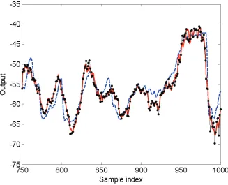
Figure 5. Model predicted output produced from the identified models of 8 and 15 model terms, over the validation data set, for the fruit fly modelling problem. The dashed line indicates the original measurements; the thin dotted line indicates the model predicted output of the 15-term model; and the thick solid line indicates the model predicted output of the 8-term model.

Acknowledgements

The authors gratefully acknowledge that this work was supported by EPSRC (UK). They are grateful to Dr M. Juusola, the University of Sheffield, for providing the fruit fly data.

References

D. M. Allen, “The relationship between variable selection and data augmentation and a method for prediction,”

Technometrics, 16(1), pp. 125-127, 1974.

A. R. Barron and X. Y. Xiao, “Discussion: multivariate adaptive regression splines,” Ann. Statistics, 19(1), pp. 67-82, 1991.

S. A. Billings and S. Chen, “The determination of multivariable nonlinear models for dynamic systems using neural networks,” In C.T. Leondes (Ed.), Neural Network Systems Techniques and Applications. San Diego: Academic Press, pp. 231-278, 1998.

S. A. Billings, S. Chen, and M. J. Korenberg, “Identification of MIMO non-linear systems suing a forward regression orthogonal estimator,” Int. J. Control, 49(6), pp. 2157-2189, 1989.

S. A. Billings and G. N. Jones, “Orthogonal least-Squares parameter-estimation algorithms for nonlinear stochastic-systems,” Int. J. Sys. Sci., 23(7), pp. 1019-1032, 1992.

S. A. Billings,S.A. and W. S. F. Voon, “Correlation based model validity tests for nonlinear models,” Int. J. Control, 44(1), pp. 235-244, 1986.

S. Chen, S. A. Billings, and W. Luo, “Orthogonal least squares methods and their application to non-linear system identification,” Int. J. Control, 50(5), pp. 1873-1896, 1989.

S. Chen, C. F. N. Cowan, and P. M. Grant, “Orthogonal least-squares learning algorithm for radial basis function networks,” IEEE Trans. Neural Networks, 2(2), pp. 302-309, 1991.

S. Chen, X. Hong, C. J. Harris, and P. M. Sharkey, “Sparse modeling using orthogonal regression with PRESS statistic and regularization,” IEEE Trans. Sys. Man, Cyber. B, 34(2), pp. 898-911, 2004a.

S. Chen, X. Hong, and C. J. Harris “Sparse kernel density construction using orthogonal forward regression with leave-one-out test score and local regularization,” IEEE Trans. Sys. Man, Cyber. B, 34(4), pp. 1708-1717, 2004b.

P. Craven and G. Wahba, “Smoothing noisy data with spline functions—estimating the correct degree of smoothing by the method of generalized cross-validation,” Numer. Math., 31(4), pp. 377-403, 1979. J. H. Friedman and B. W. Silverman, “Flexible Parsimonious Smoothing and Additive Modeling,”

Technometrics, 31(1), pp. 3-21, 1989.

J. H. Friedman, “Multivariate adaptive regression splines”, Ann. Statistics, 19(1), pp. 1-67, 1991.

G. H. Golub, M. Heath, and G. Wahha, “Generalized cross-validation as a method for choosing a good ridge parameter,” Technometrics, 21, pp. 215-223, 1979.

W. Gonzalez-Manteiga, A. Quintela-del-Ro, and P. Vieu, “A note on variable selection in nonparametric regression with dependent data,” Statistics & Probability Letters, 57(3), pp. 259–268, 2002.

X. Hong, P. M. Sharkey, and K. Warwick, “A robust nonlinear identification algorithm using PRESS statistic and forward regression,” IEEE Trans. Neural Networks, 14(2), pp. 454-458, 2003.

X. Hong, M. Brown, S. Chen, and C. J. Harris, “Sparse model identification using orthogonal forward

regression with basis pursuit and D-optimality,” IEE Proc. Control Theory and Applications, 151(4), pp. 491-498, 2004.

J. H. Z. Huang and L. J. Yang, “ Identification of non-linear additive autoregressive models,” J. Royal Statistical Soc. Series B, Part 2, 66, pp. 463-477, 2004.

A. J. Miller, Subset Selection in Regression. London: Chapman and Hall, 1990.

R. Myers, Classical and Modern Regression with Applications (2nd _{Ed.). Boston: PWS-KENT Publishing}

Company, 1990.

P. Stoica, P. Eykhoff, P. Janssen, and T. Söderström, “Model-structure selection by cross-validation,” Int. J. Control, 43(6), pp. 1841–1878, 1986.

M. Stone, “Cross-validity choice and assessment of statistical predictor,” J. Roy. Statist. Soc., 36(2), pp. 111-147, 1974.

D. Tjostheim and B. H. Auestad, “ Nonparametric identification of nonlinear time series: selecting significant lags,” J.Amer. Statis. Assoc., 89(428), pp. 1410-1419, 1994.

P. Vieu, “Order choice in nonlinear autoregressive models,” Statistics, 26(4), pp. 307-328, 1995.

H. L. Wei, S. A. Billings, and J. Liu, “Term and variable selection for nonlinear system identification,” Int. J. Control, 77(1), pp. 86-110, 2004.