Seismic soil structure interaction

Sc:>

i

c:::

I ri. t ~ ::i:-a.

c:::

i

by

ZHAO X i ri.gqu._a..ri.

A thesis submitted in partial fulfilment

of the requirements for the Degree of Doctor

of Philosophy at the University of Canterbury

Abst.:ra..ct.:

A time domain analysis procedure and computational models for seismic

soil-structure interaction are presented in this work. The time domain

analysis technique makes it possible to take the nonlinearity of the soil and

the_upper structure into account in the soil-structure interaction analysis.

The boundary element method has been used to model the far-field soil

which has been shown to be very effective for a surface foundation or an

embedded foundation in a linearly elastic half space, A simplified vertical

energy transmitting boundary has been developed for a large near-field in

which nonlinear finite elements are used. This simplified vertical boundary

requires much less computational effort than that required by the boundary

element method because no numerical transformation is required,

The bounding surface plasticity model has been implemented for the solid

finite elements of the near-field soil and the beam elements of the upper

structure. This model can also be used in the free field analysis.

An approximate model for the far-field dynamic stiffness matrix has been

proposed for the time domain analysis. By specifying the dynamic stiffness

matrix of the far-field at the fundamental frequency of the soil-structure

system, a nonlinear analysis of the near-field and the upper structure can be

performed. Techniques to avoid the unstable solution of the approximate model

are also given.

Various partitioned analysis procedures are discussed and a numerical

evaluation of the stabilities and their accuracies are presented.

An primary investigation of the soil-structure interaction effects is

performed for two sites. Period shift due to the presence of the flexible

soil has a very strong influence on the structural responses and the large

structural displacements relative to the free field caused by the

soil-structure interaction were found to be responsible for the pounding of

adjacent structures. The soil nonlinearity has been found to be an important

A c kr.t.<.>"\i\7"1 e <lgemeri. t:

This research was carried out at the Department of Civil Engineering,

University of Canterbury under the overall guidance of Professor R. Park, the

Head of the Department.

I wish to thank Dr. A. J. Carr, the main supervisor of the research

project, and Dr. P.J. Moss, the co-supervisor of the project, for their

invaluable advice and encouragement which have been of fundamental importance

in completing this work.

Thanks are due to Dr. A. Bhimaraddi and Dr. R.O. Davis for their

invaluable discussions.

Thanks are also due to Professor Gao Boyang

~

}j] )

Shen Shizhao (

y,br,t~)

Institute, Harbin, for their support and encouragement.

Grateful thanks are extended to the academic staff and fellow

post-graduate students for their assistance. Special thanks are given to Mr. B.

Hutchison for his assistance on the computer work and Mrs. V. Grey for her

drawing.

I am yery grateful to the Sisters in Villa Maria for their generous

support, especially to Sisters Anne McLaughlin, Murry George, Marian Maxwell,

Joan Kinney, Juliana Gallagher, Liguori Fox and Benedict Mcquillan.

I express my sincerest gratitude to Mr. J.B. Dunne for his most generous

support and the arrangement of the accommodation.

Special thanks are due to Dr. Yan Hui Wang for her invaluable support

and a great deal of encouragement.

The deepest gratitude is given to my parents for their precious support

T ~ b l e o f C o ~ t e ~ t s

Abstract . . . ; . i

Acknowledgement ii

Table of Contents iii

Table of Principal Symbols . . . vi

Chapter 1

1.1 1.2 1.3 1.4 1.5 Introduction

Soil-Structure Interaction Effects in a Seismic

Environment

General Analysis Procedure

The Basic Governing Equation of Equilibrium

of the Soil-Structure System . . . .

Modelling of the Near-Field Soil and the Upper structure

Modelling of the Far-field Soil

Boundary

Energy Transmitting

1.6 Prospects for a Feasible Analysis 'Procedure

on Available Computers

Chapter 2

2.1

2.2

2.3

The Theoretical Development of an Energy Transmitting

Boundary - - Boundary Element Method . . . .

The Basic Wave Equation in an Infinite Domain

Dynamic Stiffness Matrix for Soil Element Discrete

Form of Wave Equations

Boundary Element Method Based on Green's Function

2.4 Derivation of the Green's Function for a Two

Dimensional Surface Foundation Resting on a

Horizontally Layered Half Space

2.5 Derivation of the Green's Function for

a Tow Dimensional Foundation Embedded

in a Horizontally Layered Half Space

2.6 An Alternative Approach to Evaluate the Global Nodal

Forces and the Local Response

2.7 A Simplified Vertical Boundary for the Finite Element

Model in the Near-Field

2.8 Summary

Chapter 3

3.1

3.2

3.3

3.4

Modelling Of the Near-Field_Soil and Upper Structure

Basic Formulation for the Finite Element Analysis

Basic Formulation of the Theory of Plasticity

Constitutive Law for the Near-field Soil

Finite Element Implementation of the Soil Model

3.5 Determination of the Model Parameters

and the Model Prediction .

3.6 The Bounding Surface Plasticity Model

for the Beam Element

3.7

3.8

Chapter 4

4.1

Solution Techniques for the Dynamic Problems

Material Assumptions and Other Available Models

Computer Implementation of the Energy Transmitting

Boundaries and Numerical Considerations

The Boundary Element Formulation . . .

4.2 Transformation in the Wave Number Domain

and the Spatial Domain . . . .

4.3 The Implementation of the Simplified Vertical

Energy Transmitting Boundary . . .

4.4

Chapter 5

5.1 5.2 5.3 5.4 5.5 5.6

Symmetric and Antisymmetric Foundation Systems

Time Domain Analysis and the Approximate

Modelling of the Far-Field . . .

Transformation of the Dynamic Stiffness Matrix

Computational Procedure for a Time Domain

Analysis Using the Convolution Integral

Previously Proposed_Frequency Independent Model

The Proposed Approximate Model and

Its Numerical Verification . . . . . . .

Numerical Results of the Simplified Vertical Boundary

Chapter 6

6.1

6.2

6.3

6.4

Chapter 7

7.1

7.2

7.3

Chapter 8

8.1

8.2

8.3

8.4

8.5

Chapter 9

Free Field Analysis and the Input Motion

for Soil-Structure System .

Free Field Analysis of a Linear Horizontally

Layered Half Space . . . .

Nonlinear Analysis of a Horizontally Layered Half Space

Evaluation of the Scattered Motion . . . .

The Seismic Loads for the Soil-Structure System

with Energy Transmitting Boundaries

Partitioned Analysis Procedure

for the Soil-Structure System .

The General Partitioned Analysis Procedure

Stability and Accuracy Evaluation

Summary

A Primary Investigation of Soil Conditions and

Soil-Structure Interaction During a Strong Earthquake

Soil Condition and Building Damage

The Response of the Structures on Stiff Soil

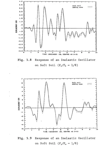
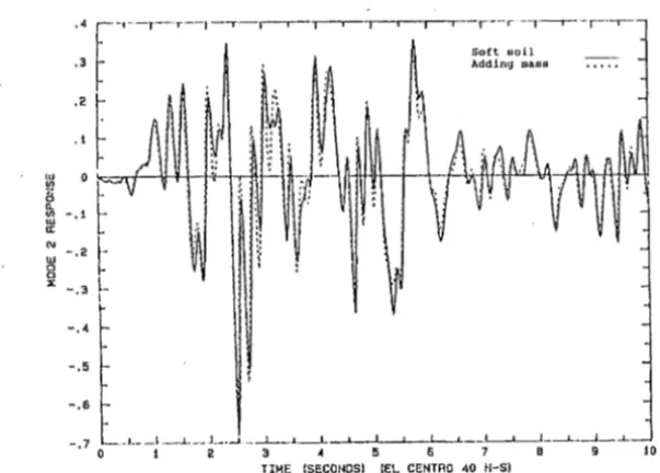
The Response of the Structures on Soft Soil

Soil Nonlinearity and Foundation Failure

Summary Conclusion 123 123 126 127 128 133 133 144 151 153 153-157 165 180 187 189

References . . . 192

Column vector.

Matrix or submatrix.

< >

a Constant for the Newmark numerical integration.

S Constant for the Newmark numerical integration,

1 Shear strain.

S1J Kronecker delta symbol.

E" Elastic strain EP Plastic strain

€~ Strain tensor.

a1J s·tress tensor.

r Shear stress or time in a convolution integral.

A Lame constant or the slope of the normal

consolidation line of soils.

~ The slope of the swelling line of soils

u Poisson's ratio.

p Mass density.

r

~ Curvature.

{~} Modal shapes.

{~} Modal shapes for a fixed base structure.

0 Beam end rotation.

w Circular frequency.

~t Time increment.

8 Partial differential operator.

V2 _{Laplacian differential operator.}

0 Rotation strain.

ry Stress invariant ratio.

AP The amplitude of incident dilatational wave.

BP The amplitude of reflected dilatational wave.

A.v The amplitude of incident shear wave.

B" The amplitude of reflected shear wave.

[CJ Damping matrix

c Phase velocity.

d

[ D

l

e

EI

f [Fl

{F}

F( ) Fr( )

[ Ffb

l

[ gu

l

[ gt

l

G H h i k K [K] L { L} [L] m M [ M] { M) N

Dilatational wave velocity.

The depth of a layer or the prefix for incremental quantities.

Forth order tensor for the elastic material's property.

Constitutive matrix.

Void ratio.

Flexural stiffness of a beam section.

Material parameter of a beam section.

Plastic modulus of a beam section.

Slope of the bounding line for a beam section.

Plastic void ratio.

Mode of the normal vector of a yielding function.

Flexibility matrix.

Nodal forces in the frequency domain.

Yielding function.

Fourier transform operator.

Flexibility matrix of the ground.

Green;s function for displacement.

Green's function for surface traction.

Shear modulus.

Plastic modulus.

Plastic modulus of the bounding surface.

Material parameter of soils.

Imaginary unit, ie., J-1.

Hardening parameter of soils.

The first stress invariant.

The deviatoric stress invariant.

The determinant of the deviatoric stress matrix.

Wave number.

Bulk modulus for soils, or plastic modulus for beam elements.

Static stiffness matrix.

Loading function.

Dilatational wave propagating direction vector.

Load shape function.

Material parameter for soils.

Material parameter for soils.

Mass matrix.

Shear wave propagating direction vector.

Unit normal vector.

(N] Displacement shape functions.

p Mean normal effective stresses of soils.

{p} Loads in the x-direction.

P Surface traction in the x-direction

q Deviatoric effective stress.

{q} Beam end displacement vector.

{Q} Beam end force vector.

r Tangent of the incident angle for dilatational waves.

{r} Load vector in the z-direction or nodal displacement vector

in the time domain.

R Surface traction in the z-direction.

{R} Nodal force vector in the time domain.

s

[ s]

[ Sfb]

[ Sfb]

[ Sbb]

t

u

Tangent of the incident angle for shear waves.

Dynamic stiffness matrix.

Dynamic stiffness matrix of the ground with excavation.

Dynamic stiffness matrix of the free field.

Dynamic stiffness matrix of the bounded near-field soils.

Surface traction or time.

0isplacement function for the x-direction in the frequency

domain.

{U} Nodal displacement vector in the frequency domain.

v Displacement function for they-direction in the frequency

domain.

w Displacement function for the z-direction in the frequency

domain.

{W} Nodal displacement vector in the z-direction in the frequency

domain.

l . l

C h a . . p t e r l

:::r:: rl. t :r c:, d. "I.I c:: t .i c:, rl.

S o i l - S t r ~ c t ~ r e I ~ t e r a c t i o ~

E f f e c t s i ~ a S e i s m i c E ~ ~ i r o ~ m e ~ t

In recent years, much research has been carried out in the field of

dynamic soil-structure interaction, especially where this has been concerned

with the design of massive civil engineering structures such as nuclear power·

plants and cooling towers (14, L5, W8, Wl2). The soil-structure interaction

effect is also recognized as being important for everyday building structures

(14, L5, W8). The presence of the deformable soil modifies the response of

the structure in two aspects. Firstly, the free-field ground motion at the

site without the structure is strongly affected (01, S7, S8). Secondly, the

presence of the structure creates another source due to the structure

interaction with the surrounding soil, ie. , the incident seismic waves

impinging on the base of the structure will be reflected and the actual base

motion of the structure is different from the free-field motion at the site.

Since the late 1950's, it has been noticed that the soil conditions at

the site have a strong influence on the ground motion during an earthquake

(S7, S8). The maximum ground accelerations developed at two sites at about

equal distances from the zone of energy release could be considerably

different from each other due to the different soil deposits~ Furthermore,

the response spectrum from the two sites could have different characteristics.

The reason for this phenomenon is that the seismic waves travel in a different

manner in different media. For example, at two sites with the same bed-rock

but different soil deposits on them, the seismic waves travel towards the

sites from a source and impinge the surface of the bed rock. Because the two

soil systems have different natural frequencies, it is very likely. that low

frequency components of the seismic wave will be amplified by the softer soil

Thus a structure with a low fundamental frequency may be severely affected

where it rests on the soft soil deposits but adjacent stiffer structures on

the same deposits may be hardly affected at all. Conversely, the structures

with low fundamental frequency on stiffer soil deposits may be only slightly

affected while . adjacent stiff structures are subjected to large inertial

loading (S7, S8).

The multiple reflections of seismic waves in a soil medium make it very

difficult to describe the seismic wave mathematically, In most seismic

engineering analyses, the soil ?eposits of the site are usually assumed to be

much stiffer than the structure resting on the soil. The reflected waves

from the structure's base are ignored. The motion that the structure's base

is subjected to is assumed to be the same as the free-field ground motion and

all of the input energy from the seismic excitation has to be dissipated by

the inelastic deformation within the structure. This is called a single

source problem. For most kinds of soil medium, the above assumption is far

from realistic.· The reflected waves from the structure carry a considerable

amount of energy away and this is referred to as the radiation damping effect.

In a layered or irregular soil medium, some secondary waves may be produced

from the reflected wave and they may strike the structure again. Thus the

response of the structure may be very different from the expected one.

Due to the presence of a deformable soil, the dynamic characteristics of

a structure change. For example, the resonant frequency is no longer the

natural frequency of the fixed base structure but the natural frequency of

the soil-structure system. Usually, the natural frequency of the

soil-structure system is much lower than the natural frequency of the fixed

base structure. In general, the presence of deformable soil will result in

a reduction of the maximum structural distortion in a seismic environment if

the fundamental period of the soil-structure system is larger than the

fundamental period of the site.

Because the rocking is permitted by a deformable soil, the vibration

modes of the structure are different from those of the fixed base structure.

For a nonlinear frame, the change of vibration modes may result in a different

plastic hinge distribution. Some of the plastic hinges originally designed

to dissipate the input energy may never be formed. The ductility demand may

example, for the bounded near-field soil and upper structure, finite element

models can be used. For the unbounded far-field soil, some other model, such

as the boundary element model may be used to incorporate the energy radiation.

The different parts of the soil-structure system can be discretized

differently according to their accuracy requirements. For example, the upper

structure is usually required to be analyzed with much more detail than the

soil and thus a finer model can be used for the upper structure (W8). When

the upper structure is modified during the design process or the system is

analyzed under a different seismic excitation, the dynamic stiffness matrix

of the far-field soil does not have to be recalculated.

If the non-linearity is restricted to the near-field and the upper

structure, the substructure procedure can still give a good approximation when

the total displacements are used as the basic unknowns (LS, W8). For most

engineering applications, the non-linearity of the far-field soil may not

affect the response of the structure very much and can be taken into account

by the free-field analysis. Since seismic wave equations derived under the

assumption of an elastic soil medium do not hold, the wave incidence and

reflection mechanism in a nonlinear soil medium is different from that in

elastic soil medium. In order to perform a nonlinear analysis by using the

substructure procedure, the same incidence and reflection mechanism has to be

assumed, ie., the seismic waves impinge and are reflected on the boundary

between the elastic soil medium and nonlinear medium in the same manner as

between tw~ elastic regions. If the boundary used in the analysis can absorb

all kinds of impinging wave completely, this assumption is realistic, because

the distorted wave impinging on the boundary from the nonlinear soil region

can be decomposed into the components in the form of the elastic waves with

different £requencies.

nonlinear soil region.

The maximum displacement relative to the free-field may increase if

soil-structure interaction is taken into account. The seismic energy may be

transferred among adjacent structures, especially where the dynamic

characteristics are different, and the structure-structure interaction effects

may be quite large (Wl3).

l . 2 G e ~ e r ~ l A ~ ~ l y s i s P r o c e < l ~ r e

Theoretically, the easiest and most logical way to perform an analysis

of soil-structure interaction in a seismic environment is to model a

significant part of the soil around the structure and to apply the free-field

motion at the artificial boundary (L5, W7). This direct procedure allows for

nonlinear soil behaviour and can result in a true nonlinear analysis if the

modelled part of soil is large enough. This problem is referred to as a

source problem with the source being the external boundary. The direct

procedure is not practical because the number of dynamic degrees of freedom

is too great for most available programs and the computational cost can be

very large. Because only a limited part of the soil can be modelled in this

direct procedure, the superposition law is often assumed to be valid. In

this case, a substructure procedure, which is computationally more efficient,

can be employed (15, W7).

If the motion of the soil-structure system is assumed to consist of two

parts, a free-field motion and the interaction motion, the analysis can be

performed by the following procedure (W8). In the first step, the free-field

motion on the interface between the structure or near-field soil, which is

the boundary of the soil being modelled, has to be computed and the analysis

of the unbounded far-field soil is carried out without the presence of the

structure. In the second step, the unbounded soil is modelled as a subsystem.

The dynamic stiffness matrix of the degrees of freedom on the interface is

determined. Then the interaction motion can be calculated by exerting the

interaction forces resulting from the free-field motion on the interface

nodes.· This is a source problem and can be solved relatively easily.

The advantage of the substructure procedure is that the upper structure,

l . 3 The B a s i c G o ~ e r ~ i ~ g E q ~ a t i o ~ o f E q ~ i l i b r i ~ m o f t h e S o i l -S t r ~ c t ~ r e -System

In order to facilitate the nonlinear dynamic soil-structure interaction

analysis, the total displacement is used in the basic governing equations.

At first, the formulae are given in the frequency domain and then transformed

into the time domain.

In the following context, the near-field soil is regarded as an expanded

part of the structure.

The equilibrium equations of the structure can be expressed in the

frequency domain as (B4, LS, W8)

· (1.1)

~here S represents the dynamic stiffness matrix, U represents the displacement

and F represents the forces applied on the structure. The superscript t

stands for the total motion, the subscripts stands for the structure and the

subscript b stands for the nodes on the boundary between the near-field and

far-field.

The dynamic stiffness matrix

(SJ

(SJ= -

[M)

+

(K]

if viscous damping is introduced, or

(SJ= -

2ri)

if hysteretic damping is introduced. Here [M], [CJ and [K] represent the

f is the hysteretic damping ratio. [S •• ], [S.b], (Sb.] and [Sbb] are subrnatrices of [

s l.

In Eq. 1.1, [Fb] is the interaction forces applied at the boundary and

depends on the structure boundary motion relative to (U~}, the motion of the

boundary nodes of the ground in which the near-field soil and the structure

are absent.' Thus it can be shown that

(1. 3)

where (Sfb] is the dynamic stiffness matrix of the ground without the

near-field soil and cannot usually be written in the form of Eq. 1.2.

Substituting Eq. 1. 3 into Eq. 1.1, the equilibrium equation of the

soil-structure system is

{(U!}}

(1. 4)

In the analysis of soil-structure interaction under earthquake excitation,

the only loaded nodes are often those on the interface of the far-field and

near-field. Often [F.] is equal to zero and the typical form of the equation

of motion is

{(if.}}

(UO

(1. 5)

The dynamic stiffness matrix of the far-field [Scb] is complex and

frequency dependent. Its real part can be interpreted as generalized spring

coefficients and imaginary part as generalized damping coefficients. It can

be written as

(1. 6)

Subs ti tu ting Eq. 1. 2a and Eq. 1. 6, Eq. 1. 5 may be written in the

( - w2

+

l

[K •• )

[Kb. l

{{U;}}

{U~}

(1. 7)

Because the dynamic stiffness matrix is frequency dependent, the

classical modes of the soil-structure system do not exist even in a 'entirely

linear system. It is still possible however to transform the structure

displacements into the modal displacements of the structure fixed at its

boundary by the following transformation (W7):

{UU (1.8a)

(U;} (1. 8b)

(U~} [<I>] ( z} (1.8c)

(1. 8d)

where {Uh} is the nodal displacement on the near-field boundary relative to

the ground motion, {U!} is the structural displacement relative to the motion

of the structure when the boundary nodal displacements are applied statically.

[T.b] is the quasi-static transformation matrix, [<I>] is the modal shape of the soil-structure system fixed at its boundary nodes and {z} is the modal

( - w2

[2[r][OJ"' (OJ

j

[(OJ

j ) r)}

+ iw

[ Cfb ( w) ] + [ 0 ]

[O] [ Kgb(w)] {Ub}

{ ['>J'[M.,J[T,,J }

- w1 {Uf} ( 1. 9)

[ Mbb] + [ T •bl T [ M •• ] [ T ,bl

where [I] is an identity matrix, [O)=[<I>]T[K •• ) [<I>], and

[n

whose elements are modal damping ratios if viscous damping is introduced.

I

Eq. 1.7 can be transformed into the time domain by the inverse Fourier

transformation involving a convolution integral (W7):

{{

r~}}

{rU

(1.10)

where

t

{ Rb ) =

J{ [

0

+[qb(t-r)]((r~(r)} - {rHr)})}dr (1.11)

where r is the displacement in the time domain and [Kfb(t)] and [qb(t)] are

the dynamic stiffness matrices of a linear far-field soil with the excavation

In most analyses, it is more convenient to use the ground motion of the

free-field to evaluate the interaction forces. Eq. 1.11 can be rewritten as

(W7)

t

{Rb}=

J< [

0

- [ K{b < t - ,,. ) J (

r: (

cib

r~

where the superscript f stands for the free-field. By using Eq. 1.12, the

scattering motion does not have to be calculated, but the relationship can be

found from the following equation in the frequency domain (W7),

[S~]

[S~)

[S~]

(1.14)

where [S~b] is the dynamic stiffness matrix of the near-field soil with only

the degrees of freedom on the interface that contacts the far-field. These

equations can be derived by using a sub-structure analysis on the soil system

without the upper structure. Because the near-field soil is a bounded domain,

its dynamic stiffness matrix can be calculated using the finite element

method.

1 . 4 - M o < l e l l i ~ g o f t h e N e ~ r - F i e l < l

S o i l ~~<l t h e U p p e r s t r ~ c t ~ r e

In the dynamic analyses of civil engineering structures, several

discretized models, such as the finite difference, the finite element and

the boundary element methods, have been successfully employed (B3, BlO, C2,

Z2). It appears that the finite element method is the most powerful one.

During the design process, the structures are usually analyzed under static

loading by the finite element method. During a dynamic analysis, an

additional matrix, which takes the inertial effect into account, is needed.

derived. The dynamic characteristics of a structure can be fully determined

by the mass, damping and static stiffness matrices and a dynamic analysis can

be performed under any kind of dynamic loading. Due to its simplicity and

accuracy, this procedure is superior to the "true dynamic" finite element

analysis in whi.ch a dynamic element stiffness matrix is derived from the

dynamic differential equilibrium equations in the frequency domain and the

mass and stiffness matrices are coupled (G2).

For the mass matrix, a different set of displacement shape functions

from those used in the derivation of the static stiffness matrix can be used

as long as all significant inertial loading can be represented and this

usually results in the lumped mass matrix. The damping matrix may be

constructed on an element level in order to introduce different damping ratios

for the different elements or on the structure level using Rayleigh or

proportioned damping for simplicity (Il).

Often a coarser dynamic model than the static model may be preferred

beca1,1se the computational cost for a dynamic analysis is too high or the

static model can not capture all essential dynamic responses and the dynamic

model has to be established by a direct discretization (W7). In all

circumstances, the discretization procedure for the near-field and the upper

structure in a dynamic analysis is very similar to that used for a static

analysis.

For the upper structure, many different models can be used. For a

structure with a simple geometry, a shear beam model may be used when all the

vertical and twisting displacements are restrained and rigid floors are

assumed. For a three dimensional frame, the rigid floor assumption can still

apply and result in a small dynamic system. For more complex structures, the

plate element, shell element and curved beam element, or combination with

some other simple element types can be used.

When a more complicated model is used, it is still possible to restrict

some less important degrees of freedom or to distribute the structural mass

to some master degrees of freedom to reduce the number of dynamic degrees of

freedom. The simplest way may be to assume zero mass on certain degrees of

freedom and use static condensation to eliminate these degrees of freedom (B3,

C2). This reduction procedure does not apply to nonlinear systems where a

For the near-field soil, many kinds of elements can be used to discretize

the domain. For example, in two dimensional analyses, even the combination

of a simple shear beam or truss element can be used which is very simple to

implement even for nonlinear analyses but may give coarse results. Usually,

two or three dimensional isoparametric finite elements are recommended in

which some sophisticated nonlinear constitutive law may be introduced.

It is worth noting that in certain linear soil-structure interaction

analyses, the use of global generalized displacements to define the structural

displacement may result in a smaller dynamic system than the finite element

model. For example, in the analysis of a tall .chimney, only the first 5 or

6 modes are needed to represent the structure reasonably well (14).

1 . 5 M o d e l l i ~ g o f t h e F a r - f i e l d S o i l - - E ~ e r g y T r a ~ s m i t t i ~ g B o ~ ~ t l a r y

In soil-structure interaction analyses, the most important and difficult

task is the modelling of the far-field soil because of its unbounded nature.

If a significant part of the soil is included in the model, the nature of the

boundary is not important because the amplitudes of the interaction waves

will be quite small when impinging on the boundary due to the material and

geometry damping. From the aspect of computational cost, only a very small

part of soil can be modelled. As described in Section 1.1, all of the

outgoing waves from the interaction between the soil medium and the structure

must travel through the artificial boundary without any significant

reflection. In previous research, many different kinds of boundaries have

been employed to incorporate the energy radiation and they can be catalogued

into three types: elementary boundary, local boundary and consistent boundary.

In the early research on soil-structure interaction, the boundary of the

model was assumed to be either fixed or totally free. All impinging waves

were reflected back into the model and the reflection resulted in a distorted

structural response. To improve the results, the boundary is usually located

far away from the structure and high artificial material damping is introduced

structure their amplitudes are small enough to give a reasonably accurate

structural response. The model leads to high computational cost and the

abnormal material damping results in erroneous responses.

In order to take the energy radiation into account, another type of

boundary has been used. Usually, the boundary consists of a series of dash

pots and springs which are coupled only between the adjacent nodes (L6, Wl).

This kind boundary is called a local boundary and usually absorbs only part

of the impinging waves. For example, a frequency independent viscous boundary

has been extensively used in soil-structure analysis (B4, LS, S5). Infinite

elements have been developed as an energy absorbing device (Ml). Many other

types of local boundary have been employed in the literature (L2, S11). The

advantage of local boundaries is that they are easy to implement with the

finite element method because they couple only the adjacent nodes on the

boundary. It can be shown that the local boundaries can completely absorb

only certain types of impinging waves from some angles.

In recent years, the boundary element method, a powerful numerical method

to deal with an unbounded domain, has been applied to structural dynamics

(BlO, S12, W3, W4, W6), The boundary element model in the time domain for an

uniform half space has been used in soil-structure interaction analyses (S12).

The boundary element model developed by Wolf is suitable for a horizontally

layered half space and can be attached to surface foundations, embedded

foundations and finite element meshes (W7). It can completely absorb all

kinds of impinging waves with varying angles of incidence. In the boundary

element model, the dynamic stiffness matrix can be evaluated in the frequency

domain or directly in the time domain and nonlinear analysis can be performed.

For comparison, the fundamental concept in both the finite element and

the boundary element method will be given, In the finite element analysis,

a given domain is discretized into finite number of elements and then the

displacement field is constructed by using certain interpolation functions

with nodal displacements as the unknown parameters. Next the boundary

conditions are imposed on the constructed displacement function. Finally,

the original differential equilibrium equations are satisfied by applying the

principle of virtual work (B3). In the boundary element analysis, the

displacement fields constructed are required to satisfy the differential

equilibrium equations of a given domain and some boundary conditions under

The original differential equilibrium equations are transformed into a set of

boundary integral equations by using Green Is functions. Now the only

requirement is that all boundary conditions have to be satisfied. The same

discretization procedure can be used for the boundary of the given domain.

Shape functions are used to construct the displacement on the boundary and

then the boundary condition is imposed in some average sense. The interior

displacement can be evaluated after all boundary unknowns are solved (BlO, W7,

W8).

For an unbounded domain, the boundary element method is superior to the

finite element method. For wave propagation problems, it is impossible to

exclude the incoming waves by the artificial boundary of a truncated finite

element mesh. Conversely, it is quite easy to derive analytical solutions

which satisfy all differential equations exactly in addition to the radiation

condition when the soil system is under certain types of dynamic loadings.

These analytical solutions can be used as the weighting functions in the

indirect boundary element procedure (W7, W8). In a horizontally layered half

space, the discrete form of the wave equations can be used to derive the

analytical solutions under some fictitious loads with unknown amplitudes

acting on the exterior of the interface between the near-field soil and

far-field soil. These analytical solutions will satisfy all of the boundary

conditions between the adjacent layers and free surface except those on the

interface. The interface boundary conditions can be imposed in some average

sense by adjusting the unknown amplitudes of the fictitious loads. Thus the

displacement and force relationship on the interface' can be determined. It

is worth noting that for a horizontally layered half space, the analytical

solution for the boundary element has to be constructed numerically.

If the near-field is modelled by finite elements and the number of the

elements on the vertical boundary is large, the efficiency of the boundary

element may be impaired because the Green's functions for all .nodes have to

be stored and a numerical transform has to be performed. The computer storage

requirement increases dramatically with the increase of the number of the

boundary elements on the vertical boundary. The required accuracy is hard to

achieve because of error accumulation in the numerical transformation. In

this case, some other kind of energy transmitting boundaries may be preferred.

For example, for a horizontally layered half space, surface wave modes may be

used to construct the transmitting boundary since most energy is carried away

be used and the error due to discretization can be minimized. The

computational cost for this boundary is much less than that for the boundary

element because no numerical transformation from the wave number domain to the

spatial domain is required. The boundary is considered as a special case of

the boundary element for the vertical boundary in the sense of the weighting

technique and numerical procedure and will be referred to as a simplified

vertical boundary in what follows.

In conclusion the boundary element method may be the best way of

modelling the unbounded domain when a linear elastic far-field is assumed.

When the discrete form of the wave equations are used, the boundary element

method can also be used for a horizontally layered half space. If linear

soil is assumed, boundary elements can be directly attached to the foundation

of the upper structure and thus no finite element model is needed for soils.

When a large part of the soil is modeled by a finite element model to take

into account the nonlinear behaviour of the soils, the partial reflection of

the outgoing waves may not induce significant error in the response of the

upper structure because of the material damping of the soil. In this case,

a frequency independent viscous boundary may be preferred for a homogenous

half space because of its simplicity and the simplified vertical boundary for

a horizontally layered half space.

l . 6 P r o s p e c t s f o r a F e a s i b l e A ~ a l y s i s

P r o c e t l ~ r e o ~ A ~ a i l a b l e C o m p ~ t e r s

In a dynamic soil-structure interaction analysis, the main computational

effort is the evaluation of the dynamic properties of the upper structure and

near-field soil, the calculation of the dynamic stiffness matrix of the

far-field soil and the solution of the system equations. Because of the

presence of the soil, the resultant dynamic system will be much larger than

that for a fixed base structure. The memory required in a computer program

will be greatly increased. In the evaluation of the dynamic stiffness matrix

of far-field soil a substantial part of the computational effort has to be

devoted to the complex transformation between the different domains, the

calculation of discrete forms of the wave equations and the evaluation of

methqd can be used either in. the frequency domain or directly in the time

domain, but some of the quantities have to be computed in the frequency domain

first and then transformed into the time domain. For example, if a time

domain boundary element is applied, the Green's function has to be computed

in the frequency domain first, as all of the discrete forms of wave equation

are valid only for harmonic motions, then transformed into the time domain

(WlO, Wll). The convolution integrals require a considerable amount of

computational effort and memory. For a realistic engineering problem, it may

not be practical to use the time domain boundary element for a horizontally

layered half space on current computers, or at least not a practical way

during the design process. It may be preferable to use the boundary element

method in the frequency domain.

For a linear system, the transient analysis may be achieved by the

frequency domain analysis for some initial conditions. For a nonlinear

system, the analysis can only be performed by employing convolution integrals

because the dynamic stiffness m~trix is frequency dependent. The· dynamic

stiffness matrix has to be computed in the frequency domain first and then

transformed into the time domain. This computation procedure reported earlier

proved to be very time consuming and the transformation was numerically very

difficult (Z2). It is attractive to develop an approximate model ,based on

the frequency domain boundary element for far-field soil applicable to

nonlinear structural analysis but with less computation effort than that

associated with the frequency domain solution.

When the boundary elements are used to model a far-field soil, the

resultant dynamic stiffness matrix has a different form from that of the

near-field and upper structure. The finite element discretization results in

strongly banded and sparse mass, damping and stiffness matrices. The dynamic

stiffness matrix from the boundary element is a fully populated matrix but

with a smaller number of degrees of freedom than for the finite element

procedure. In the solution procedure, it may be not very efficient to solve

the combined system equations because the resultant system have mixed

characteristics. It may be more effective to use a partitioned analysis

procedure which has been used successfully in fluid-structure interaction

analysis (F2, PS). When an approximate model is used for the far-field soil,

Cha..pte:r 2

T h e T h e ~ ~ e t i ~ ~ l D e ~ e l ~ p ~ e ~ t ~ f

~~ E ~ e ~ g y T ~ ~ ~ s ~ i t t i ~ g B~~~d~~y

B~~~d~~y E l e ~ e ~ t M e t h ~ d

2 . l T h e B a s i c Wa~e E q ~ a . . t i o ~

i ~ a ~ I ~ f i ~ i t e Doma..i~

Wave propagation in an elastic medium is the fundamental problem of

dynamic soil-structure interaction. For the sake of completeness and

readability, the three dimensional wave equations in cartesian coordinates are

given below (W7).

In the following expressions Cartesian tensor notation is used because

of its simplicity in writing. The subscript indices (1,2,3,) represent

(x,y,z) respectively.

The Kronecker delta symbol will be used,

if i=j

otherwise

The summation convention will apply, ie.,

au au+ au+ au

and

When a body is under a harmonic excitation with frequency w, the

equilibrium equation of an infinitesimal rectangular parallelepiped

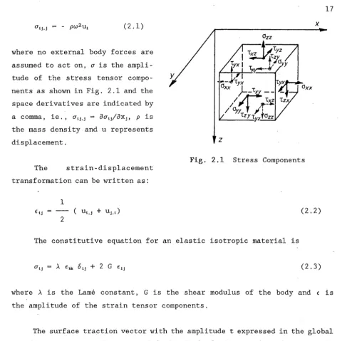
(2.1)

where no external body forces are

assumed to act on, a is the

ampli-tude of the stress tensor compo- Y

nents as shown in Fig. 2.1 and the

space derivatives are indicated by

a comma, ie., a1J,J = 8a1J/8xJ, p is

the mass density and u represents

displacement.

The strain-displacement

transformation can be written as:

1

2

X

z

Fig. 2.1 Stress Components

(2.2)

The constitutive equation for an elastic isotropic material is

(2.3)

where A is the Lame constant, G is the shear modulus of the body and e is

the amplitude of the strain tensor components.

The surface traction vector with the amplitude t expressed in the global

coordinate system acting on an infinitesimal element can be related to the

element stress by the unit normal vector of the surface, ie.,

(2.4)

Substituting Eq. 2.2 and Eq. 2.3 into Eq. 2.1, the following equation can

be obtained,

(2.5)

Now three displacement components can be solved by taking the boundary

conditions into account. The prescribed surface traction can be enforced by

To solve Eq. 2.5, two displacement components have to be eliminated and

the resulting differential equation is, however, of fourth order. An

alternative way of solving for the displacement is to introduce new variables:

the volumetric strain with amplitude e and the rotation strain vector (O} with

the amplitude components 01 , 02 and 03 • They are defined as

e = Eu (2.6)

\1

( U3,2

-

2

1

( U1,3

-

2

1

( U2,1

-

2

The four unknowns can be uncoupled by a simple elimination procedure.

It can be shown that the following two equations are achieved,

w

'v2 _{e e (2.8)}

cP

W.

v2

-

c.

where 'v2 is the Laplacian operator, cP is called the dilatational wave

velocity and is specified as

Cp = [ A + 2G ] ;~ p

c. is called the shear wave velocity and is specified as

(2.10)

(2.11)

The wave equations Eq. 2.8 and Eq. 2.9 are linear partial differential

equations of the second order.

iw iw

exp (- sP ) exp (iwt) (2.12)

.(2.13)

where {L)T =[Lx, Ly, L,], {XF =[x, y, z], sP is the coordinate measured along

a straight line in the propagating direction and Ap is a constant.

It can be verified that the trial solution satisfies Eq. 2.8 if the

following condition holds,

1 .(2.14)

The thtee scalars can be considered as the direction cosines of the straight

line along which sP is measured.

The corresponding amplitudes of the displacement components are

SP

LJ AP exp [iw (t - - - ) ]

Cp

where the subscript j x, y, z indicates the direction.

From Eq. 2.15 and Eq. 2.14 it can be shown that

SP

AP2 exp [ 2iw (t - - - ) ]

Cp

(2.15)

(2.16)

Eq. 2.16 represents a scalar wave propagating in the positive SP-direction

with the velocity cP and amplitude Ap. Its displacement vector coincides with

the direction of propagation. At a given time t = t0 , the displacement vector

is constant if sP is constant, ie. , on a plane perpendicular to the

propagating direction, the displacement vector is constant. The wave

represented by Eq. 2.15 is called a dilatational wave or P-wave and subscript

p has been introduced to indicate the wave type.

The following analogous trial solution can be used for Eq. 2.9,

iw iw

(0) - {C} exp (- s. ) exp (iwt) (2.17)

(2.18)

where (M}r = [Mx, My, M,], (C)r = (Cx, Cy, C,] and s. is the coordinate measured

along a straight line in the propagating direction.

The condition for Eq. 2.17 to satisfy Eq. 2.9 is

(M)T (M) 1 (2.19)

(M)T (C) 0 (2.20)

The three components of {M} are the direction cosines of propagation and (C}

contains the amplitudes of the rotation strains.

The corresponding displacement components are

s.

A,J exp [iw (t - - - ) ] (j x, y, z) (2.21)

c.

in which

(2.22a) ( M~ + M~ )1;2

A.y = - - - (2.22b)

( M~ + M~ )1;2

(2.22c)

c.

(2.22d) ( M~ + M~ )1;2

A,v (2.22e)

( M,_2 + My2 )1/2

where A.h is the amplitude of the horizontal component and A.v is the amplitude

of the component lying in a plane determined by the vertical axis z and the

direction of propagation. It can be shown that Eq. 2.21 represents a wave

propagation with the constant velocity c •. This type of wave is referred to

as a shear wave or S-wave.

In most engineering applications, it is reasonable to assume that the

P-wave and S-wave propagate in the x-z plane. Substituting Ly= My =·0 in Eq.

2.15 and Eq. 2.21 and adding the displacement caused by the P-wave and the

S-wave, the total displacement components are

u = u(x,z) exp (iwt) (2.23a)

v = v(x,z) exp (iwt) (2.23b)

w = w(x,z) exp (iwt) (2.23c)

SP S8

u(x, z) = Lx AP exp (-iw - - ) + M, A,v exp (-iw - - ) (2.23d)

s.

v(x,z) A,h exp (-iw - - ) (2.23e)

c.

Sp S1

w(x,z) L, AP exp (-iw - - ) + Mx A,v exp (-iw - - ) (2.23f)

c.

L~ + L~ 1 (2.23g)

1 (2.23h)

Lxx + L,z (2.23i)

s. = Mxx + M,z · (2.23j)

where u, v and ware the displacement components in x, y and z direction

2 . 2 D y ~ a r n i c S t i f f ~ e s s M a t r i ~ f o r

S o i l E l e r n e ~ t - - - D i s c r e t e

F o r m o f Wa~e E q ~ a t i o ~ s

In a horizontally layered half space, the displacement solution has t'o

satisfy all of the boundary conditions between the adjacent layers and at the

free surface. This requirement makes it impractical to derive an analytical

solution for the layered half space. Instead, each layer can be treated as

a single element and the solution can be constructed for each element and the

boundary conditions can be imposed in the same way as in the finite element

method.

In the following sections, only the in-plane motion is considered because

the out-of-plane motion is much simpler and the further details may be found

in the reference (W7, Kl).

The general definition of the stiffness matrix is the transformation

matrix relating the force components and their corresponding displacement

components. The dynamic stiffness matrix of a soil element will relate the

stress amplitudes on the boundary to the corresponding displacement

components. To enforce the boundary conditions at the top and bottom of the

layer, the following condition has to be satisfied (Kl, W7)

Lx Mx

(2.24)

ie., the P-wave and the S-wave have the same variation in the x-direction.

To solve for L, and M, from Eq: 2. 23g and Eq. 2. 23h when L,., which equals the

cosine of the P-wave incidence angle, M,, which equals the cosine of the

S-wave incidence angle, are known, two roots with opposite signs for L, and

M. can be found. They represent the waves travelling in the opposite

direction. All of these waves have to be included in the solution of the wave

equations.

CP c.

C = (2.25a)

L.: M,,

w

k (2.25b)

C

1

r = - i ( 1

-

L.:

1

s = - i ( 1

-

M,,

where c and k are the phase velocity and wave number, respeqtively.

Substituting Eq. 2.25 into Eq. 2.23d and Eq. 2.23f and including the reflected

waves travelling in the positive z-direction, it can be shown that

u(z,x) u(z) exp (-ikx) (2.26a)

w(z,x) w(z) exp (-ikx) (2.26b)

AP

r"]-

(2.26c)

A.v

w(z) -Lreikrz Lre·ikrz -Meiksz -Me •ik••

B,v

where L and M are Lx and M,, , respectively. AP' BP' A.v and B.v are the

amplitudes of the corresponding waves. Eq. 2. 26c can be written symbolically

as

(U(z)) [GU(z)] (A) (2.26d)

Substituting Eq. 2.26 into Eq. 2.2 and Eq. 2.3, the stress functions a.,

and r"' can be derived as

a .. (z,x) a,.(z) exp (-ikx) (2.27a)

r(z}

= ikG

r ,..(z) 2Lreikrx -2Lre•ikrz M(l-s2 )eiksz M(l-s2 )e•ikn

(2.27c)

ie.,

(2.27d)

Setting u(z) = U1 and w(z) = W1 when z = 0 and u(z) = U2 and w(z) = W2

when z = d where dis the depth of the layer, and substituting these into Eq. 2.26c then

U1 L L -Ms Ms AP

iW1 -iLr iLr -iM -iM Bp

(2.28a) U2 Leikrd Le•ikrd -Mseiksd Mse•iksd A.v

iW2 -iLreikrd iLre•1krd -iMeiksd -iMe•iksd _B.v

ie.

[GA] {A} (2.28b)

and

(U(z)) (2.28c)

The stresses are then determined from

Applying the same procedure to Eq. 2.27c but setting P1

at z = 0 and P2 = r.,2 , R2 = a,.2 at z = d leads to

P1 -2Lr 2Lr -M(l-s2) -M(l-s2)

iR1 -iL(l-s2) -iL(l-s2) i2Ms -i2Ms

ikG

P2 2Lreikrd -2Lre-ikrd M ( 1- s 2 ) e iksd M( 1- s 2) e-iksd

iR2 iL(l-r2 )eikrd iL(l-r2 )e-ikrd -i2Mseikad i2Mse-iksd

i.e.,

{P} [PA] {A}

AP

BP

(2.30a) A.v

B.v

(2.30b)

After solving Eq. 2.28b for (A} and then substituting {A} into Eq. 2.30b,

the dynamic stiffness matrix of the soil element can be obtained where

( p) _(2.31)

(2.32)

The matrix inverse in Eq. 2.32 may be performed analytically and the explicit

form of the dynamic stiffness matrix of a soil layer for in-plane motion is

given in the appendix with some special cases.

The above procedure is very similar to the finite element procedure and

the function

+co

[Nu(z,x)] =

J

(2.33)

may be interpreted as a displacement shape function which satisfies the

differential equilibrium equations exactly.

For a half space, applying loads at the free surface will only develop

the waves travelling in the positive z-direction. The radiation condition

requires that no waves come toward the free surface from infinity. Setting

AP and A.v equal zero in Eq. 2. 26c and using the similar procedure eliminating

BP and B.v lead to the dynamic stiffness matrix of the half space' [ sp-sv"] . The complete form is given in the appendix.

For a loaded horizontal layer, the equilibrium equation of an

infinitesimal element can be expressed as (W7)

(2.34)

where p1 is the loading function. For in-plane motion, all of the variables

concerned with they-direction can be omitted.

expressions are assumed

If the following loading

{p(z,x)} = r(z,x)

{p'(Z)}

r(z)

(2.35a)

and the load is linearly distributed in the vertical direction

z z _P1

rz]

d d ir1

(2.35b)

z z _P2

r(z) 0 -i(l - - ) 0 -i

d d ir2

the particular displacement solution of Eq. 2.34 is (W7)

c2

.

.

rz]

1 r2c~ d kdr 2s 2 c2 p

k 2G i c2 s i z

WP( Z ), - - ( 1

-

-)

kdr2s2 c2 _p s2 d

zd

.

(1- - )

dr2c~ kdr 2s 2 c2 _{p ir1}

(2.36a)

i c2

.

-

-

where p1 and p2 are the load amplitudes at z = 0 and z = d acting in the

x-direction, respectively, and r1 and r2 are the load amplitudes at z = 0 and

z =din the z-direction respectively, ie.,

[ PU( z)] { p} (2.36b)

Substituting Eq. 2.36 into Eq. 2.3, letting P1 = - 'Tx.i, R1 = - a •• 1 , P2 = 'Tu2 and

R2 = a •• 2 , the dynamic stiffness matrix for the linearly distributed loading is

1 kd -1 0

G kd(2-d/ct)

diet

[SP] (2.37a)

d -1 0 1 -kd

0 -eve% -kd(2-cVc%) cVc%

and

[ SP

l

Material damping can be taken into account by introducing complex

material properties, ie., hysteretic or viscous damping is assumed. As a

result G , cP and c, may be replaced in all of equations by (LS, S 2; W7)

G* = G ( 1 + 2

r.)

c*

.

c* p

Cs ( 1 + 2 rs) 112

for hysteretic damping and

G*

c*

.

c* p

G (1 + 2wL)

c. (1 + 2wr .)1/2

(2.38a)

(2.38b)

(2.38c)

(2.38d)

(2.38e)

(2.38f)

for viscous damping, where

rp

r.

2 . 3 B o ~ ~ t l a r y E l e m e ~ t M e t h o d B a s e d

o ~ G r e e ~ ' s F ~ ~ c t i o ~

In an elastic domain where no body forces are assumed to act, which

satisfies the differential equilibrium equation Eq. 2.5, the displacement

solution under a set of loads which satisfies all boundary conditions is a

Green's function for this set of loads.

To present the principle of the indirect boundary element method used in

the following section, a one-dimensional problem shown in Fig. 2.2 is taken

as an illustration.

Spring

Ks

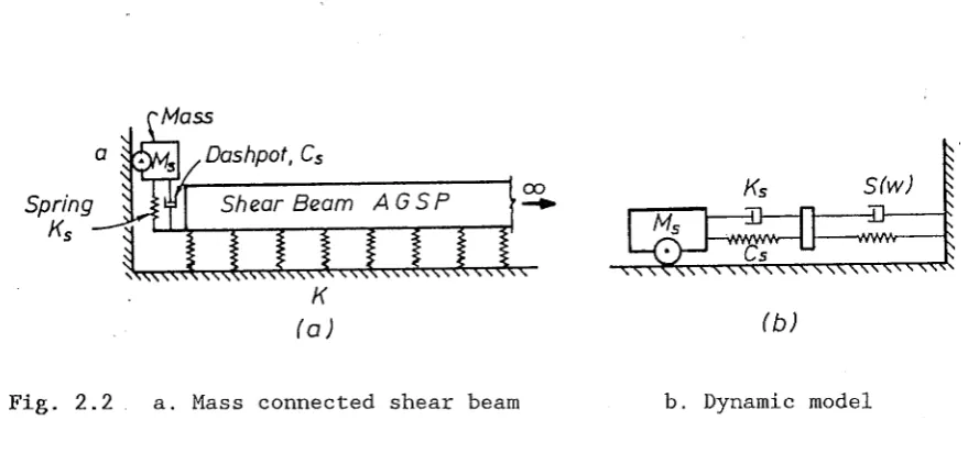
Fig. 2.2

K

(a)

a. Mass connected shear beam

(b)

b. Dynamic model

A mass is connected through a spring K. and a dashpot

c.

semi-infinite shear beam with shear area A, shear modulus G, cross section

area Sand mass density p resting horizontally on an elastic foundation with

spring constant·k. If the shear beam is under a harmonic excitation at its end

(x = 0) with amplitude P, the equilibrium equation in the vertical direction

is represented by

k

w -

w

w

GA c2 ₈

C. -- [ ~ ] 1/2 _(2.39c) pS

where

Q

satisfies the boundary condition W(x) = 0 at x = oo is

W(x) a exp (-iwx/c) (2.39d)

where c is the wave velocity, i.e.

[

r~

C = w

k(a.

-

(2.39e)

w GA

(2.39f)

c. k

aw

= - - exp(-iwx/c) (2.39g)

ax

Q(x) -iGAw a/c exp (-iwx/c) (2.39h)

If W(x) W0 at X 0 then

Q(x) -iGAw/c W0 exp ( -iwx/c) (2.39i)

The dynamic stiffness coefficient of the shear beam under a point load is

s

For an infinite beam with the same properties under a point load with an

unknown amplitude q at x = - e, the equilibrium equation is

k

W,xx - - - W + - - W q &(x+e) (2.40a)

GA c2

.

W(x) i

Q(x)

qc

exp (-iwe/c) exp (-iwx/c)

2GAw

q

2

exp (-iwe/c) exp (-iwx/c)

which can be referred to as the Green's functions.

(2.40b)

(2.40c)

By enforcing the

displacement W(x) = W0 at x = 0 , the unknown load amplitude can be solved

from Eq. 2.40b.

q - 2 ( GAk( l-a.2) )112_{exp ( iwe/c) W0 (2.40d)}

Substituting Eq. 2.40d into Eq. 2.40c and setting x = 0, the relationship

of the force and the displacement at the end can be specified as

p _(GAk(l-a02) )112

w.

s

The stiffness coefficient of the beam is identical with the analytical

solution because in enforcing displacement boundary conditions, no

approximation is introduced.

For a three dimensional half space, the stiffness matrix of the far-field

soil can be derived using the indirect boundary element method in a similar

procedure to that for the semi-infinite shear beam. Firstly, distributed

loads with initially unknown intensities are assumed to act on a source

boundary S' which is offset toward the far-field soil in the semi-infinite

domain without excavation because the analytical solutions are available for

this domain (W3, W4, W7). In the limit, the source boundary can be moved

toward the interface S between near-field and far-field up to an infinitesimal

distance. Because only a finite number of loads can be chosen, an

interpolation function [L(s')] has to be selected and an approximation is

introduced. The distributed load can be expressed as a function of unknown

nodal values {p),

where s' is the coordinate measured along the source boundary S' . The

displacement and surface traction on the interface S for the semi-infinite

domain under the load p(s') can be calculated, .

(Up(s)} (2.41b)

(Tp(s)} [gt< s)

l

where s is the coordinate measured along the interface S and gu(s), gt(s)

contain the elements of Green's function.

Secondly, the prescribed displacements on the interface can be

constructed as

(U(s)} (2.41d)

where [N(s)] is the interpolation function and {Ubl is the nodal displacement

vector.

Finally, the displacement boundary condition on the interface S has to

be enforced by the weighted-residual technique

J[W(s)r((U(s)) - {Up(s))) ds

s

(2.4le)

where [W(s)F contains the weighting functions. From Eq. 2.4le the unknown

loads at all nodes can be determined. The weighting functions can be chosen

in different possible form according to the different error distribution

mechanisms. Here the matrix of the Green's functions [gt(s)] is chosen as

the weighting function. From Eq. 2.4le, following equations result in

[G]{p) [Tl {Ub} (2.41£)

[G] J[gt(s) ]T[gu(s) ]ds (2.41g)

s

[T] J[gt(s) JT[N(s) ]ds (2.41h)

The concentrated nodal forces on the interface can be obtained as

(Ph}=

J

s

(2 .4li)

Substituting Eq. 2,41c and Eq. 2.4lf into Eq. 2.4li the force-displacement

relationship can be found as

<2.4lj)

The stiffness matrix of the far-field is

(2.41k)

It can be verified that matrix [G] is symmetric and that the stiffness matrix

is always