Stably layered fluids

(1)

A thesis

submitted for the degree

of

Doctor of Philosophy in Mathematics

in th

University of Canterbury

by

A.K. Laing /

/

University of Canterbury Christchurch, New Zealand

(2)

LIBRt,RX'

(3)

Chapter

ABSTRACT

I INTRODUCTION .•

II CRITICAL POINTS IN THE FLOW OF A LAYERED

III

FLUID FROM A RESERVOIR

§2.1. Theory

§2. 2. Solu ons

§2.3. Results and Discussion

§2.4. Generalisation

SOME FURTHER FEATURES OF CRITICAL POINTS

§3.1. Association of erjtieal points

with erfaees ..

§3.2. Relation of critical Unsteady flouJs

ints to

IV PERMANENT WAVES IN A CLOSED THREE LAYERED

v

FLUID

§4.1. Background

§4.2. The general equations

§4.3. Single mode equations

§4.4. Permanent waves in onemo

PERMANENT WAVE STRUCTURES

§5.1. The equations

§5.2. The method of solution

§5.3. Results

§ 5. 4. Cone Zusion

(4)

ACKNOWLEDGEMENTS 123

REFERENCES 124

(5)

ABSTRACT

Various problems associated with a stably layered fluid are studied.

Firstly, the flow of a layered fluid from a reservoir is considered. Steady solutions are sought and found to depend on the flow at the critical points, that is, points at which the long wave speeds for the different modes of gravity wave propagation vanish. For certain distributions of the layers' depths i t is found that there are too many critical points, and hence the flow is overdetermined and no steady solutions are possible. Thus, when reservoir conditions are slowly altered so as to pass from one depth ratio to another, the flow will not necessarily change slowly too.

A closed three layered fluid with small density differences between the layers is also studied. The

non-linear interactions between the two, closely related,

internal wave modes are investigated, and general evolution equations are obtained for small disturbances at the inter-faces. Permanent solutions involving one mode alone are calculated, but i t is found that at certain wavelengths

the slower mode permanent waves resonantly generate harmonics of the faster mode.

When the group velocity of a train of faster mode waves is the same as the phasevelocity of a slower mode wave there is significant interaction leading to a permanent wave

(6)

(7)

CHAPTER 1

INTRODUCTION

This thesis deals with various problems associated with a stably layered fluid. In general the systems

considered comprise a rigid lower boundary with homogeneous layers of fluid arranged in order of decreasing density and bounded above by either a free surface or a rigid lid.

The most important areas within these fluids are the regions of density discontinuity, or the interfaces, and i t is here that a disturbance within the fluid will manifest itself. If a free surface is considered an interface whose upper layer is of zero density, then a system with n inter-faces will allow n different modes by which a given

disturbance may propagate. Each of these n modes has an associated long wave speed. Hence, a long wave could propagate at any of n speeds.

(8)

Froude number is unity then the flow is critical, and i t is in the regions of critical or near-critical flow that most of the interesting problems lie.

For a fluid with variations of the flow speed in the direction of flow, there arises the possibility the fluid passing through critical conditions at some points. These discrete points are called critical points and play an important role in solving the flow. If the flow is backed up by an infinite reservoir and there is a smooth geometry of contraction of the flow channel, then there will be

steady downstream increase in flow velocity and a number of critical points may exist. For a steady system WOOD (1968 and 1970), WOOD and LAI (1972a and l972b), and LAI and WOOD

(1973) provide examples of the use of critical points in solving flows. BRYANT (1974), and BRYANT and WOOD (1976) further developed this idea and applied i t to a situation in which steady flow solutions are bounded by unsteady regions in which the theory predicts and excessive number of critical points. Chapter two is an application of the same techniques to a slightly more complicated structure, and there are several different features revealed.

The question of critical points is continued into Chapter three to clar both the role of critical points in unsteady flows, and the association of critical points with the interfaces.

(9)

ined identities of the modes in internal/surface systems. The latter part of this thesis concentrates on the

non-linear theory of the system with two internal modes. The close relation of the modes causes effects not evident in studies where the interacting parts are W€11 identified such as in the interactions between waves with vastly different modes of propagation.

The aim of this nonlinear analysis is ultimately to seek waves of permanent form which may exist within this system. Permanent waves and permanent wave structures are indeed found with features definitely attributable to the closely related, internal nature of the two modes.

As with the earlier part of the thesis, the problem is historically derived from flows of a critical nature. The concept of permanent waves began with the discovery of solitary waves, that is, isolated pulses with constant shape. The wavelengths of these "solitons" is effectively infinite and they travel at speeds near the longwave speed [in actual fact the speed is {g (h

+a)}~

where h is the fluid depth and a the amplitude of the wave] which characterises the critical conditions for a fluid. In other words, if a fluid contains a critical point, then a solitary wave would be stationary and permanent in form near that critical point.

The theory of permanent waves originated in the reconc iation of two distinct classical treatments of gravity waves on homogeneous, incompressible, irrotational

fluids~ Defining a, ~ and h as scales of amplitude,

(10)

are based on the two parameters E

=

a/h and ~

=

h/~. The first is an initially infinitessimal theory involving

expansions based on the small parameter E(~ ~2). This can be Fourier analysed and to a first approximation describes linear dispersive wave motion. The other method is the long wave (or shallow water) theory for which v2 (~ E) is

the small parameter. Distortion and breaking of waves are features of this approach. However, when E/V2

₌

_{0(1) these} effects attain a balance, and waves whose shape is conserved can exist. Initial investigations were pursued in this field by SCOTT-RUSSELL(l844), BOUSSINESQ (1871), RAYLEIGH (1876) 1

and KORTEWEG and DE VRIES (1895) .

The Korteweg -de Vries equation which describes the evolution of waves under these conditions has been found relevant for many physical problems besides small1 finite

amplitude water waves. These include: Magneto-hydromagnetic waves in cold plasma; Rotating flow in a tube; Pressure waves in liquid gas bubble mixtures; Ion accoustic waves in an

anharmonic crystal; Longtitudonal vibrations of a harmonic discrete mass string; and Longtitudonal dispersive waves in elastic rods [see KRUSKAL (1974) for references].

One of the features of the Korteweg -de Vries equation is that i t accommodates solutions of permanent form.

Internal waves of permanent form were not considered until much later [KEULEGAN (1953) 1 LONG (1956)] when

(11)

(1966), using a flow force perturbation expansion, provides a generalised theory for internal permanent waves allowing arbitrary vertical density and velocity distributions, and either a free upper surface or a rigid upper boundary.

The interaction of different wavetrains has long been a topic of interest, particularly in oceanography. The concept of radiation stress was used by LONGUET-HIGGINS and STEWART (1960) to study the effect of a wavetrain of

long waves on another of short waves. The variation in energy of the short waves is found to correspond to the work done by the longer waves against the radiation stress

the short waves. This study has later been extended to a two layer system with a surface to see the effect of long interfacial waves on a wavetrain of short free-surface waves [GARGETT and HUGHES (1972)]. The drawback of this method in relation to the present study is the prescribing of the long waves.

However, the present approach is based on a general method proposed by BENNEY (1966) for studying long

non-linear waves and their interactions without prior knowledge of the wave profiles. Generalised expansions in both

parameters E and ~2 are found and solutions sought in the

neighbourhood of E

=

~2

=

0. Korteweg -de Vries type

(12)

In the present study several features make BENNEY'S approach preferable to BENJAMIN'S.

Benjamin's analysis is primarily a steady flow analysis based on an expansion of the wave resistance in a small

displacement parameter s. The problem then yields solutions which are shown to be derived from the O(s2) terms. Such solutions are of necessity permanent in form.

However, Benney's method is initially an unsteady

expansion of the general problem. Thus, evolution equations can be found for which solutions of permanent form are

special cases. This method provides a better basis for studying non-linear wave interactions since the notion of wave propagation is present until the final step.

The former approach retains very close contact with its physical interpretation. However, mathematically the flow force is regarded as an integral equation to be solved by successive approximation. On the other hand Benney

writes partial differential equations for the non-linear perturbation equations. These can be solved using fairly standard techniques, and generally seem more manageable than integral equations.

One development incorporated in the present study is that used by BRYANT (1973) [and in subsequent papers] where the wavelength parameter ~ is unrestricted, and so

the expansion is in terms of s but allows a wide range of ~. This ~-exact approach means that Stokes' waves,

(13)

give the evolution of the interfacial amplitudes.

The significance of the non-linear effects incorporated into the analysis is in the quadratic interactions they

represent between the various wave harmonics present. These interactions are particularly significant if resonance or near-resonance occurs. If k is a wavenumber, and w(k) the associated linear frequency of a wave, then the resonance conditions for quadratic interactions require that

kt

'+

k2

+

k3

=

0

w ( k 1 ) + w ( k2 ) + w ( k3 )

=

0 •

(1.1)

( 1. 2)

In the presence of more than one mode of propagation the frequencies may be of any mode, hence a wide range of

possibilities is present. For near-resonance the relation in (1.2) is a near equality in which case there is still an appreciable transfer of energy possible between elements of the near-resonant triad - For a conservative system, at resonance the energy within a triad is conserved but can be readily transferred between the component harmonics.

For a closed three layered system there are two inter-faces and two internal modes for wave propagation. The non-linear interactions between harmonics of both modes and their contribution to the formation of permanent waves and groups of waves with permanent envelopes are studied in chapters four and five. Chapter four concentrates on developing the relevant evolution equations and using these to solve for permanent waves consisting of one mode only or predominantly one mode. Chapter five extends this to

(14)

(15)

CHAPTER II

CRITICAL POINTS IN THE FLOW OF A LAYERED FLUID FROM A RESERVOIR

The properties of critical points are instrumental in solving certain types of flow. If a layered fluid flows with uniformly increasing velocity in the downstream

direction, and the correct number of critical points exists, solutions for the flow can be found at these points and

consequently anywhere in the fluid. At the critical points the geometry of the channel containing fluid determines the flow. Hence the naming of the critical points as

controls.

WOOD (1968) analysed the flow from a stably-layered reservoir through an open channel with a horizontal

contraction. The method he established was used later for various reservoir outlet problems including: lock exchange flows (WOOD 1970), layered fluid flow over a weir (WOOD & LAI 1972a) , layered fluid flow from a

reservoir into a closed conduit {WOOD & LAI 1972b), and two-layered flow through a contraction (LAI & WOOD 1973). The critical point corresponding to the fastest wave mode, which occurs at the point of minimum width, is called the control, whilst the upstream critical points are called virtual controls.

(16)

conduit that if the withdrawal is steady there may be

discontinuous changes to the flow ratios between the layers. In fact, for some configurations i t is shown that no steady solutions exist, whilst for others there is the possibility of more than one solution. The involvement of critical

points is all important and this chapter further investigates this role using a slightly more complicated model. The work was begun as part of a Masters Thesis by the author (1975).

Consider a large Reynold's number (inviscid), non-diffusive, stably layered fluid, flowing in the positive-x direction through a smooth horizontal contraction with a point of minimum width at x

=

0. A weir is placed in the contraction so that its maximum height is at x

=

0.

Assume the flow is backed up by a reservoir so that the time for a fluid particle to travel through the contraction is small compared to the time for the streamline patterns to change. This is effectively a system of steady flow with reservoir conditions that can be prescribed. Also assume the hydrostatic approximation, which is reasonable provided the reservoir outlet's dimensions change only gradually so that vertical accelerations are negligible compared to horizontal accelerations.

§2.1. The aim of this chapter is to explore the involvement of critical points in the limiting conditions for steady solutions of a reservoir outlet flow regime. Mathematically, for a stable system there is a fixed number of critical

(17)

However,there are situations in which an excessive number of critical points tends to form and so cause

over-determination of the system, and hence instability.

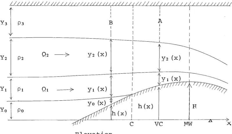
Consider the system depicted in figure (2.1) with two flowing layers above a third stagnant layer. Both the height and width of the channel are functions of x and the geometry of the channel is determined by the relation

h(x) + b(x)

=

a constant, where b(x) is the channel width and h(x) the height of the weir above some datum. The flowing layers are represented by the subscripts 1 and 2 for lower and upper layers respectively, whilst the non-flowing layers by 0 and 3. The thicknesses of layers are yi, the fluxes Qi, the velocities ui,and the densities

0) is H.

This system has three main points of interest: a control at the point of minimum width (MW) which is also the weir crest, a virtual control (VC) somewhere upstream at x

=

xVC' and a point of contact between the lower

interface and the weir (C) which is also upstream of

(18)

I

I I 11!/11/111 ///l!/111/111/llll!:///l I /(l/lll!/(;1111 I I t !1/1!11111 I I

I I I I

I I

Y3 P3 B I ~ I

I 1 I I

I I I I

I I I

I I

I

Y2 (x)

(x)

Y 1

l

P1 Ql ----7> Y1 (x)

Yo

I

Po

Yo _h(x)

vc

MW

Elevation

MW ---~~---~

Re s e r v o i r ----,---?>

Plan

b(x)

2

-Figure 2.1

Geometry is b + H

=

b + h m

I

[image:18.595.102.502.101.332.2]

(19)

The flow regime may be subdivided into two types: flows with the virtual control upstream or downstream of the point of contact respectively (xvc 5xc). The regions with lxvc - xc

I

small are of particular interest since the proximity may well influence the solutions. In this section the model is analysed theoretically. A discussion of

possible experimental situations is included in the presentation of the results in §2.3.

§2.1:1. Firstly consider xc

<

xVC

<

xMW'

The energy equations at the interfaces yield ~ Y2 G:f =Yo +Y1 +Y2 -y1 -y2 -h

· 2 · ₁ P2 3 2

~ Y1 G1 = "'2 Y2

p-;:-;

G2 +Yo +Y1 -y1 -h

( 2 ._1)

( 2. 2)

where p .. = p. - p. and G. 2 is the dimensionless quantity

l J l J l

2

p. Q.

l l

(j 3 if i _2' j 2 if i 1) . gb 2y ~ ( p . - p . ) =

=

l l J

Clearly further equations are required, so the condition that the layers must vary smoothly is used. Differentiating equations (2.1) and (2.2) and solving;

1 db

=

_b

_dx

_rn-;T'

I

D1

I

=

_b

1 db _dx

_m

I

b dx 2

xvc·

invoke the finiteness condition on dy1 _and _dy2

dx dx

To

requires that either

~~

= 0 or ID1 [ = ID2 I = 0 at the critical points.

db

Obviously at the control dx

=

0 and so we must have that

D1 and D2 are also singular at the virtual control.

[Notes: (1) An unsteady analysis of the same configuration would give long wave speeds vanishing under the same

condition of singularity of Do. Briefly, the characteristic directions for unsteady propagations (xk) are defined by

singularity of a coefficient matrix D(x); so [D(x)

I

=

0. Now xk corresponds to the long wave speed of one of the interfacial modes, and thus, for steady flow, the points

.

at which x

=

0 correspond to the critical points. This is born out by the observation that [D(i = 0) I = 0 =} [Do I = 0.

This relation between the characteristics and critical points is clarified in Chapter III.

(2) Do, D1, and D2 differ only in one column.

Given that [oil

=

0 for any two i E {0,1,2} then, means that [D.

I

will vanish for all i E {0,1,2}. Hence,

smooth-l

ness of y. gives only two independent conditions at the

l

virtual control,

I Do I = I D1 [ = 0.] .

Thus far: at VC,equations (2.1) and (2.2) along with

I Do I

=

I D1 [

=

0 ;

at MW,equations (2.1) and (2.2) along with

I

Do

I

=

0;

(21)

. 2 .

QQ__!_ _{(Yo -h)} ₀

-y1G1 -

=

p 1 2

or Po 1 (Yo -h) + P1 2 (Yo + Y1 - Y1 -h)

+ P2 3 (Yo + Y1 + y2 - h- Y1 - Y2)

=

0 ( 2. 5)

are the equations.

The first seven of these at VC and MW are sufficient to solve for 01, Q2, ylVC' y 2VC' ylMW' Y2MW and hvc (or xvc), and once these have been obtained the final three equations at c will give Ylc' y 2c and he.

Consider now the limiting conditions for this type of flow. If the model is solved for various levels of the upper interface while the other external parameters are held constant, a dependence of this type of solution on the interface level is deduced. The higher the interface, the further downstream the contact point and the further upstream the virtual control. (This is true for most

cases although exceptions are found later.) In the region of small three alternatives are suggested:

( 1)

I

xc - xvc

I

vanishes with no discontinuity to the

solutions and so there is continuity between the solutions with xc

>

xvc and those with xc

<

xVC' at lxc - xvcl

=

0.

(2) Critical conditions are reached at C or some point upstream of C while VC and C are still distinct.

(3) As lxc - xvcl vanishes, c ceases to exist and this regime is "continuous" with a regime of three layers flowing.

(22)

continuity at C is unlikely. This was indeed verified by the results. The other possibilities may be tested as follows:

(2) By calculating the "critical matrix", analogous to Do , for the three layer region upstream of C and evaluating its determinant as x +x .

_c

If a point upstream of C becomes critical while x

<

xc, then C will become super-critical with respect to this speed (or mode) and testing this determinant for a change of sign at C will suffice.

( 3) By calculating dyo at C over a range of interface

dx

levels. If, as the interface rises,

dJ~

passes smoothly through zero at C, while conditions are still subcritical with respect to this mode, then the lower interface must become tangential to the weir, and the third layer begins to flow. By the same token, given a three-flowing-layer regime and a falling interface, at this point the third layer will cease to flow.

Note that as the third layer flows a third wave mode forms with an associated critical point which appears at C. So C is critical with respect to this new mode, but still subcritical with respect to the second mode

considered above.

The above tests necessitate setting up equations for the region x

<

xc:

~ Y2

Gi

=

Yo

+

Yt

+

y2 -Yo - Yt - Y2 -h ( 2. 6)

p 1 2 2 2

+ .e..u_ (Yo + Yt -h) ( 2. 7)

Yt-- Gt _p23

=

Y2 G2 -Yo - Yt P23

-yl.e..u..

Gt

₌

£.Q_!_ (Y 3 -Yo -h) . ( 2. 8)

(23)

Differentiating, 2 l-G2 Gg. 0

=

1

Pt 2 (1-Gl)

P23

Ptz 2

Pz3 Gz

2 1 db

GzY2 - - -_b _dh 1

1 cly2

dx

£.u.

dyl

Pz3 dx

E.!LL

dyo

P23 dx

1 db E.ll. 2 . £!!..!_

- b

dh Pz3 Gt Yt - _P23

dh

dx · ( 2. 9)

Thence, dJ; is readily found, and since Ylc' y

2C, and he

are known, dd·Yo

I

can be calculated. Furthermore, the x x=x

_c

matrix on the left hand side of equation (2.9) is the

"critical matrix" to be tested fo~ singularity at C. Call this D. Note that the flow will be subcritical upstream of C, so lnl

>

0 in the reservoir, and so at c,

In!

will decrease towards zero as lxvc - xcl becomes small.

These calculations therefore suffice to give the nature of limiting conditions to this type of flow.

What might happen physically in case (2) above requires a little speculation. Since xc and xvc are distinct, three critical points are implied for a two-moving-layer fluid. This flow is overdetermined and no

steady solutions exist. Some breakdown must occur.

(24)

Thus, if these solutions, for which

_<

_xvc·

_<

_x _are MW' referred to as "type A" solutions, the range of interface levels over which they exist will be bounded by low upper interface levels where cessation of flow in layer 1 occurs, and also by high interface levels where (2) or {3) above occurs.

§2.1:2. Now consider xVC

<

xc

<

xMW'

At the point of minimum width equations (2.1), (2.2) and lno

I ;

0 hold, while at the virtual control the equations

are {2.6), (2. 7) and (2.8),-w·hich after imination of

Yo -yo give

2 2 Pt 2

!:2 Y2 G2 + !:2 Yt

Gt--Po 1

=

Yt +Y2 -y1 -y2

k P t 2 Po 2 G 2 k G 2 ;

2 Y t ~

POI

1 - 2 Y2 "'2 2..!..2_ (Y1 -yt).

P23 ferentiating,

2 l-G2

=

l _ Pt 2 ·G 2 1 1

P12 02 P12

-Pz3 ot P23

1 db

b

Call the matrix on left hand side of equation {2.12) then the critical condition at

vc

is

IB I

=

0 and the finiteness conditions on dyl dyz give

dx ' dx

2 2

1 - Gz Gt Y1

=

Gi

2 . _{Po 2 .} . 2

Gt

Po 1 - G2Y2

(2.10) (2.11)

(2.12}

B,

(25)

Solutions can be found from equations (2.10), (2.11) and (2.13). [Note that the matrix D from (2.9) can be written using elementary row operations as

0 B

xc, x

t

xvc·]

Again the limiting conditions for this type of flow are sought. For various levels of the upper interface dyo

I

and !Do j are calculated.

dx x=xc x=xc

becomes small, provided !Do

I

<

0, there will be well-determined solutions.

Call this type of solution, for xvc

<

xc

<

xMW' a "type B" solution.

§2.2:1. Solutions to the type-A problem in §2.1.1

cannot be found analytically if the problem is to be kept general. For a similar situation WOOD & LAI (1972a) manage to decouple the crest equations (at MW) from the virtual control equations by setting hvc as zero, making the datum unknown, and proceed to solve analytically at VC. Thence a numerical method obtains solutions at MW and finally

(26)

the equations at C (viz (2.1), (2.2) and (2.5)) and MW (viz (2.1), (2.2) and

Jno

I

=

0) have to be solved

simultaneously. For this purpose a Newton-Raphson numerical method is used once the equations have been analytically reduced as far as possible. Once solved, the conditions at C can be found from equations (2.9), (2.10) and (2.11) with

Yo

=

0.

§2.2:2. For the type-B problem in §1.1:2

notice that there is no explicit h(x) dependence at VC

(unlike the type-A problem for which this is quite evident). The number of unknowns is reduced by virtue of the fact

that Qi and x in the form of b(x) always appear together as The equations can be decoupled and analytical solutions found at VC from equations (2 .10) ,. (2 .11) and (2 .13).

G2 _ R

From ( 2. 13) "2 - _{1 + R + y ,}

yR'

(l+y) (R+R') - R where y

=

=

y₁ [ (l+a) (R+R') - R] (l+R+a)

Y2 ~- (l+R)[2a(R+R') +R'] +a2 (R+R') '

(27)

where a= y , and also

Consider now any x

[ (l+a) (R+R1

) - R]

(l+R+ a)

xc.

Since

g~

is a constant, then

2R

a Rl [ (l+a) (R+R') - R] _(l+R+a)

Also from equations (2.6), (2.7) and (2.8)

(

uJ~

_Yz _R' R(Yt-yd + (R+R') (Yz-yz)

(l+R) (Yt-Yt) + {Yz-yz)

(2.16)

(2.17)

Using (2.16) and (2.17) and writing ~

=

,

we eventually

Y1

get

( a - S) • { ( a+ S) ( 1 + R+ a) [ R 1 _{+a ( R+ R}1

) ] + ~ ~ [ ( a 2 +aS+ S 2) •

(R+R') (l+R) + aS(a+S) (R+R1

) + (a+S)R' (l+R)

+ aSR'

J }

= 0. (2.18}

The only physical solution to this is a =

S,

so

=

== a. (2.19)

This result in fact is true for all x

<

x

_c

since equations (2.16) and (2.17) are quite general for the type-B situation.

At MW any attempts to solve analytically become too

involved algebraically and numerical computation is necessary. The ratio in (2.19) does not hold at MW or for any

x

>

xc.

These results are not surprising as the type-B situation is very similar to the two layer selective withdrawal problem for which WOOD (1968) found self-similar solutions with

Yt constant throughout. However for points downstream of C the flowing layers come into contact with the weir and this

(28)

§2.3. Results and Discussion.

It is useful to present the results in the light of

experimental possibilities and so a hypothetical experiment

is considered. Assume all the external parameters are held

constant except Yt and Y2. The upper interface is allowed

to drop. This is achieved by allowing free draining over

the weir but replenishing the upper layer in the reservoir

to maintain a constant depth. BRYANT (1974~ allowed control

over all three layers whilst BRYANT & WOOD (1976) preferred

complete draining with no replenishing. However, the models

all represent reservoir outlet schemes and thus some inflow

is likely. Hence, replenishing the upper layer to keep

constant depth is considered acceptable although, from the

laboratory point of view, less readily reproduced than

complete draining.

The varying parameter as the interface falls is taken

as Y2, which increases. Firstly the ranges of Y2 for

solutions of both type-A and type-B have been found. This

was done for a variety of values of R and R' to show the

effect of density difference ratios on the limiting conditions.

Figures (2.2), (2.3) and (2.4) show the ranges of Y2 for

which these solutions exist for the geometries with crest

heights H

=

0.5, 0.6 and 0.7 respectively. Note that all

heights and depths are measured as proportions of

Yo

(29)

-p:;

II

-p:;

[image:29.597.73.807.114.550.2]

(30)

[image:30.596.72.802.102.553.2]

(31)

[image:31.600.61.804.57.538.2]

I /

/

I

,l

00 0 0

.

0

""'

N 0 0 0 0

.

0 0 Figure 2 of .4 Y2 for Type-A o -0 and Ty e -.2 and H

~

P -B solut· 0.7. lons toe

. X1St

(32)

critical point, by (-·-·-·) if three-flowing-layer solutions are continuous with the two-flowing-layer solutions, and by

(-··-··-··) when the lower layer ceases to flow because Y1

has become too small.

Several features are notable:

(1) Lowering the crest height means the values of the density difference ratios for which the problem is of interst are higher. Since Boussinesq fluids are of most interest and p3 is taken as being very small (even p3

=

0

for a free surface), then the smaller R and R' are, the better. Subsequently the configuration with H

=

0.7 will be used in preference to the others.

Several solutions were also obtained for reduced Yo

(down to 0.1), but the effect of this was the same as lowering the crest and nothing ext~a was revealed.

(2) In every case for small lxc - xvcl the limiting factor was the tendency to form an extra critical point. It thus follows that in each case there will be an unsteady break-down of the flow pattern at the boundary (to the

two-flowing-layer regimes) for which the virtual control and contact point are close.

(3) For the type-B solutions there are two regions. If

Y2

<

0.445, 0.440 and 0.430 (in Figures (2.2), (2.3) and

(2.4) respectively), xvc increases as the interface drops, whilst for Y2 larger than these values, xvc decreases.

(33)

ranges of Yz for which type-B solutions exist.

If Yz E (0, 0.06),xvc increases with Y2 , but for

Yz E (0.77, 0.80), xvc decreases as Y2 increases.

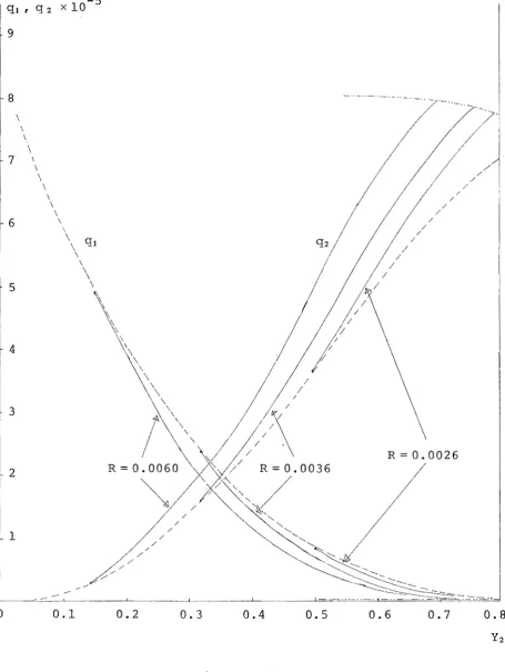
Figure (2.5), which has been included to show the dependence

of xvc and xc on Yz, makes these distinctions clear. This

figure is drawn for the three density difference ratios

R

=

R'

=

0.006, 0.0036 and 0.0026. For the first two values

the two regions of type-B solution are distinct, whilst for

the latter value they are continuous, meeting at a point

where hvc (and hence xvc) reaches a maximum.

This phenomenon is accountable if the experimental

situation is considered. Firstly, i t is reasonable to

assume when one of the flowing layers is shallow that

proportional changes in velocity for a small drop in the

upper interface are small compared to the proportional

changes in the layer thicknesses. That is, for velocity

u and thickness y, you~ uoy, so for purposes of small

change in layer thickness assume the velocities in the thin

layers are constant. Secondly, given the long wave

approx-imation, the narrower any layer becomes, the slower the

critical speed becomes (assuming the layer velocities

constant) . This of course refers to the slow mode since

the fast mode's critical point is at MW. [This is a

general comment. For example, the two layer system with

layer depths y 1 ·and y2 confined between rigid planes, has

a single mode with wave velocity proportional to

1/ (

P1 coth ky1 ·

+

Pz coth kyz) . In the long wave limit and

(34)

h(x)

0.4

0.2

0.2 0.4 0.6

R

=

0.0060

0.4

0.2

R

=

0.0036

0.4

0.2

R

=

0.0026

Figure 2.5

Positions of Virtual Control (VC) and Contact point (C) for various

levels of the upper interface. Both types of solution are included

[image:34.595.59.549.56.764.2]

(35)

decreases. For two layers with a free surface and a rigid base the smaller of the two modes' speeds (in the long wave

limit and with y 1 + Y2 a constant, say 1) is

{

Pt P2 _

Yt Y2

[p1pi _

4

(p

2

2 + P1P2) (

- y y· Pz Pt

Yt Y2 1. 2

which also decreases for either y1 or y2 small. This case is akin to the present situation.]

Thus, at the beginning of the "experiment" the interface is still high and Y2 small, so the critical speed is slow and the critical point well upstream. As the reservoir drains the interface drops, and Y2 increases with an increase in the critical speed and a downstream movement of xvc towards the contact point at xc. At the other end of the scale, as Y2 becomes large, Y1 is small and decreasing. For small enough

Y1 the critical speed will be slow again and the critical

point well upstream, getting further upstream as Yt

diminishes.

This means two regions of type-B solutions exist, as (xc -xvc) will be large enough depending on Yt or Y2 being small enough. For some parameters the critical speed never becomes sufficiently large (as the interface drops) for xVC to be close enough to xc for a breakdown. In this situation the type-B solutions are continuous but with a reversal in the direction of xvc· This is the case for R

=

R'

=

0.0026 in figure (2.5).

(36)

equations (2.12), using (2.16) and (2.19}, as

lsi

=positive constant •

IG{-

a(R+~~;+R'

I

·IR~

(l+R+R'

}G~

- {l+R+a}

I·

(2.20)

Upstream and immediately downstream of xVC the second factor on the right hand side of equation (2.20) is negative and so for a given x = x0 , as a varies the sign of the first factor in (2.20) will determine the sign of IBI and hence whether x0

2 aR'

is upstream or downstream of xvc· If G1 (a;x) and a(R+R')+R' are both sketched versus a and x in a three dimensional

figure, is not too difficult to establish that for x small enough, IBI 0 when a some a0 or when a ~ some a1 , and where IBI

=

0, xVC is respectively increasing and

decreasing.

One further point worth noting is the overlapping

type-A and type-B solutions in figures (2.2), (2.3} and (2.4}. This implies that for some interface levels in certain

distributions of the external parameters, both regimes may exist. Under experimental conditions the actual form of the solutions would probably be determined by the flow history. That is, as the interface lowers, the type-B solutions will most likely persist until breakdown occurs at the upper limits depicted in the diagrams. Similarly if the overlap were approached in the opposite manner, the type-A solutions would be expected to continue until their lower boundary is reached.

Thus, beginning with small Y2 and allowing the system

to drain, maintaining constant total depth, if only two

(37)

of the point of contact and steady type-B solutions will exist. As Y2 increases a point is reached where steady solutions no longer exist. The flow becomes overdetermined due to the presence of an extra critical point. In the diagrams this is represented by the gaps between regions of type-B and type-A solutions. Where the external parameters lie in one of these gaps, no steady solutions exist and as Yz traverses these values unsteadiness prevails. For larger

Y2, type-A solutions, with the critical point now upstream of the point of contact, appear. This brings a return to

steady flow and these solutions continue until the interface drops so far as to cut off all flow in the lower layer.

If, for small Y2, three layer flow exists, then as the upper layer drops, the third critical point will move

downstream to the point at which the lowest layer stops flowing. Here, the third critical point vanishes, and a point contact between the lower interface and the weir appears with the lower interface tangential to the

surface of the weir. Two layer flow of type-B ensues, and as Y2 gets larger there is either an unsteady transition

to type-A solutions as before, or the possibility of overlap in which case type-B solutions are most likely to persist. The transformation of the third critical point to a contact point, or vice versa, is evident in the results by

simultaneous vanishing of dJ; and the determinant of the critical matrix for three layer flow, whilst the two layer

flow matrix remains non-singular.

(38)

the upper interface by replacing the second layer only, then at low levels of the interface solutions of type-B could exist. However, i t should be noticed from figures (2.2),

(2.3) and (2.4) that this upper branch always overlaps with either one layer flow or type-A solutions. Raising the

interface would bring about either an unsteady breakdown and reversion to one layer flow or type-A flow, or a steady transition to three layer flow, depending on the parameters Rand R'. Assuming that the flow history governs the form of solution where overlapping occurs, upper branch type-B solutions are unlikely to be encountered if the upper inter-face is falling since type-A solutions will persist with a possible transition to single layer flow.

As this is a model for a reservoir outlet, there is considerable importance in the discharges for each layer. For solutions within the steady type-A or type-B regions small changes in the external parameters are reflected in small changes in the discharges. However, as the unsteady boundaries to these regions are crossed the flow ratios cannot necessarily be expected to change smoothly and slowly. In the regions of unsteady solutions the flow ratios also oscillate unsteadily.

The dependence of flux on the upper interface level is plotted in figure (2.6). The nondimensional quantities

and g)

=

P₂₃g (Yo + Y 1 + Y2 ) 5

(39)

9 8 \ \ \ \

7 I

\ \ \ \ 6 5 4 3 2 1 0 \ \

\ ql \ \ \

\

\,

\\

I

\ \ \ \ \ \ \

R = 0.0060 R=0.0036

/ / 0.1

~

/ / / 0.2 / / / / / / /

[image:39.595.68.524.35.641.2]

0.3 0.4

Figure 2.6

0.5

-

.. _

/

R=0.0026

0.6 0.7 0.8

Fluxes in both flowing layers as functions of the upper inter-face level. The fluxes are plotted only for the ranges in which type-A solutions exist. The lower limit of Y2 for a given

R(= R') is denoted by---, and the upper limit by- .. - .. - .. as

(40)

(41)

(42)

for q 1 are used. Figures (2.7) and (2.8) plot

1

R q2 and

R

q1 respectively for H

=

0.7.

The regions of overlap and discontinuity in these

diagrams can be easily identified with those in figure (2.4). For a given ratio R (and R') the solid lines are traversed from left to right. _{For small values of Y2 the best picture} is obtained from figure (2.8), whilst for large Y2 figure

(2.7) is best. The description of the experiment is the same as made previously. Note

~ flux requires evaluation of q 2

that an expression for total

P ~ k

+ (R - 2 )

ql .

For most cases Pt

likely to be considered experimentally p 3 "" 0, Pt "" 1 and

. ~ k ~·

Pt "" P2 , so that q 2 + R 2 q 1 would suffice.

§ 2. 4. Generalisation.

As a conclusion to this study a general n-layered situation is discussed. Number the layers from 0 to n

+

1

(43)

from 0 to n. Layers 0 and n + 1 are non-flowing. The method

for dealing with such multilayered systems is derived from

that of WOOD (1968). The energy equations evaluated

upstream of the contact point of the lowest interface and

the weir (Co) give the ferences

.I

yi

-hJ k

=

1,2,.o. n-1,

1=0 .

(2.21)

the upper most interface

(2o22)

r

and for the lowest interface

-~ P1 uf

=

g(Po- Pt) {Yo -yo -h). {2o23)

There are no geometrical restrictions except for the shape

of the channel and weir, for which h =h(x) and b =b(x) with

dh

=

~~

=

0 at x

=

0, and the invariance of the quantities

n+l

I

Y.

0 1

n+l

and

I

y. +h.

i=O 1

dy. Also used is the condition that the derivatives d :

i

=

0,1 o o . n + 1 must be finite, that is, that yi must

vary smoothly.

Differentiating equations (2.21) -·(2.23),after using

2

h b . . 2 - Qk h

t e su st1tut1on uk- b2 yz , we ave

(44)

Coo Co 1 0 0

Cto Ctt Ct2 0

where Coo

=

g (Po - P 1 ) . 2 .

Cot

=

Pt Qt

(Po - Pt )g _dx +

dk

=

g(pk-pk-1)dx + dh

0

0 • • • 0

c _{n,n _}

=

d n

pkQ~

k 11 2 1 • • •

~ yk

k

₌

11 2 1 • • •

9,

=

₁₁₂1 • • •

k

=

1 1 2 1 o • •

2

Pt Qt db

b3y; ·dx

2 2

[pk+1 °k+1

p~Q~J

b3 yk+l

-

b Yk

k

=

_{1 '}2 ' • • •

(45)

and d

n

From equation (2.24) we have dy.

l

dx

=

jDij db

lDf

dx i

=

0,1, . . . n

where D is the n+l x n+l matrix on the left hand side of

(2.25)

(2.24) and the D. are obtained by replacing the ith column of

l

D with the vector on the right hand side of (2.24).

Upstream of Co , D is singular at no more than n - 1 points. These are critical points or virtual controls at which the

long wave velocities of the slower modes vanish.

Downstream of Co the equations (2.21) - (2.25) all hold with the adjustment made that all terms subscripted with 0

are omitted. From D and D. form the n x n matrices E and E.

]_ l

respectively by omitting the first row and column. E is

singular at no more than n- 1 points between Co and the crest

of the weir. These are the remaining virtual controls corresponding to the points where the faster mode long wave velocities vanish. E also is singular at x

=

0 which

is the control and corresponds to the fastest mode. At x

=

0 the finiteness condition is clearly satisfied as

~~

=

~~

= 0, but at the virtual controls downstream of C we require that the E. matrices are also singular. By an argument similar

]_

to that preceding equation (2.4) this results in two independent conditions at each virtual control, viz

jEj

=

jE.

I

=

0 for any one i E {1,2, . . . n}. Similarly at

l

(46)

flow is exactly n - 1 since only then is the system well determined. In principle there can be upton -1 critical points in each part of the flow and so i t is easy to conceive how the total number in both parts of the flow upstream of x

=

0 could exceed n - 1. The flow would then become

over-determined, solutions would fail and the flow become unsteady. Gradual alteration of the interface levels causes the virtual controls to move, and as any one of them approaches C0 this type of overdetermination is likely. The resulting

unsteadiness would ist until steady solutions are again possible. The new solutions would be characterised by the appearance of one of the virtual controls on the side of C0

opposite to that i t occupied prior to the breakdown.

Thus, steady alteration of inter levels results in a progression of steady phases, in which the flow ratios change smoothly, punctuated by unsteady periods as the virtual controls pass through C0 •

The above discussion assumes layers 1 to n are all flowing, but i t is possible for the lowest layer to stop. In this case C1 will form at the position where the virtual

control corresponding to the appropriate mode vanishes. The situation is now exactly the same as before except that n -1 layers flow with n- 2 virtual controls (in steady flows) and the relevant contact point is now C1 •

(47)

(2) The analysis was for steady flow so that when an interface level is altered and the virtual controls move etc, the change in the layer depths is slow enough so that the time for the streamline patterns to change is very large compared to the time for flow through the outlet.

(3) As the flow enters the contraction, the speed in each layer increases and the points of critical speed will be progressively passed until at the control the flow becomes completely supercritical. It would seem plausible that critical conditions pertain to particular interfaces and an association can be made between each critical point and an interface. However, is shown in chapter III that this assignment is very weak and throughout the preceding chapter any such associations have been avoided.

(48)

CHAPTER III

SOME FURTHER FEATURES OF CRITICAL POINTS

The preceding chapter raises some interesting questions.

The importance of critical points in solving steady flows

has been displayed and i t would be useful to investigate any

dependence unsteady flows may have on similar phenomena in

order to generalise the concept. Furthermore, for a

multi-layered system as encountered in chapter two there are

several critical points possible, and the question arises

as to whether any correspondence can be assumed between

particular interfaces and particular critical points.

§3.1. Association of Critical points with Interfaces.

It has already been noted in chapter one that a critical

point in a steady flow is a point at which the speed of a

long wave relative to the flow becomes equal to the speed of

the flow itself, so that disturbances emanating from

some-where downstream of a critical point cannot propagate

upstream. For an n-layered system contracting downstream

as in the example of chapter two, there are n wave modes

possible and n critical points. There is a one-to-one

correspondence between the possible long wave speeds and

the critical points, since if the wave speeds are ordered,

<

C , as are the critical points,

n

<

xn (flow is in direction of increasing

x), the fastest mode, C , will be associated with x and so

n n

(49)

inter-face is the same as association of a long wave speed, and hence a wave mode, with an interface. Consequently a relatively simple multilayered system with no contraction can be used to seek a definite pairing of modes and inter-faces.

YIH (1965 Chapter 2 §12.4) considers that this

association is not ambiguous and is possible if the wave speeds

c.

are known as functions of the density

discon-1

tinuities 6pi. If Ck vanishes with 6pk then the mode whose speed is Ck belongs to the interface whose density difference is 6pk. In principle this is all very well but the associa-tion is dependent on limiting condiassocia-tions as the 6p. vanish.

1 From a practical point of view a simple comparison of amplitudes of the modes at each interface should give results valid everywhere.

Consider three uniform layers of fluid bounded above and below by rigid barriers with decreasing densities

P1

>

P2

>

P3 and undisturbed depths h1, h2 and h3,as

depicted in figure (3.1). Let the interfacial disturbances be n and ~ at the lower and upper interfaces respectively, and introduce a potential function for each layer

¢. i = 1,2,3. Then the equations are 1

'i7 2¢1 = 'i7 2 ¢z = 'i72 ¢3 = 0, ( 3. 1)

with the boundary conditions

3<h - ₀ _{on y} ₌ _ht ₊ _h2 ₊_h3 _{( 3. 2)}

ay-3</lt

= 0 on y

₌

0

-a-y

3¢2

= Dnj ·- Dnl = 3¢2 on y = h1 + n

ay

Dt 1 Dt 2

--a-y

3¢2

(50)

n(x,t)

Pt

[image:50.595.75.532.72.752.2]

I /Ill/ /Ill 11!1117TT711/IIl/17 7 TT!7TTI/Ill t/ Ill/ 11/777 TTTl/117111/11/Ti y

=

Q

Figure 3.1

and from pressure continuity at the interfaces

Pt = Pz on y = ht

+

n

Taking a first approximation, neglecting terms in squares and products of

n,

C

and <Pi i

=

1,2,3, and their derivatives

d <I> 1

= an

+

h2 ( 3 • 7)

at

a t

(51)

Thus,

cp.(x,t)

₌

R{F j (y) exp i (kx-wt)} for j

=

1,2,3

J

n (x, t)

₌

R{b exp i (kx-wt)},

~(x,t)

₌

R{a exp i (kx-wt)}.

Substituting into equations (3.2) - (3.4) eventually yields

S

= -[

(P1 - P2 )gk - W2 (P2 coth kh2

+

P1 coth kh1)] . sinh kh2

I

P2 w2 ( 3. 8)

where there are two values of the frequency w given bv the

positive solutions of the dispersion relation

[ ( p 1 - P2) gk - W2

( P1 coth kh1 + P2 coth kh3 ) ]

X ( P2 - P3 ) gk - W2 ( P2 coth kh2 + P3 coth kh3 ) ]

=

pf w4

sinh 2_kh2 ( 3. 9)

viz: W1 (k) and wz (k) where w1

>

Wz. These are the frequencies

of the two natural modes.

The ratio in equation (3.8) is convenient and represents

the ratio of amplitudes at upper and lower interfaces for a

given mode. Let r 1 (k)

=

S

when w

=

w1 (k) and r2 (k)

=

S

when w

=

w2 ( k) .

A little manipulation of equations (3.8) and (3.9) gives

the relation

=

( P _{(P2 - P3) .}1 - P2 ) (3.10)

It is instructive to realise that equation (3.9) describes

a composite system comprising

(i) the upper boundary and interface with p1 +p2,

(52)

(ii) the lower boundary and interface with p₃+p_{2 ,}

These systems individually have the respective frequencies

~ when w

=

w2 (k) .

b2

To convincingly associate a mode with an interface requires that one interface is consistently affected most by one mode. In other words, for the fast mode to be associated with the upper interface requires that

(53)

slow mode to belong to the lower interface requires that

lr 2 (k)

I

<

1 always.

Reference to equation (3.10) shows i t is convenient to

consider the relationships of lr 1 (k)

I

and lr2 (k)

I

to

(~~

-:::_

~~

J , since there is no great loss of generality 1n

choosing ( P1 :... P2)

= (

P2 - P3) and thus relating these ratios

to unity.

Firstly note that

(1) For k -+ oo, that is, very short waves, the solutions to

w~

equation (3.9) give _2: -+ P1 - P2 or P2 - P3 where if i

=

1

gk P1 + P2 P2 + P3

the limit is the larger ratio and if i

=

2 i t is the smaller.

Also from equation (3.8)

(. ) I (

P1 :... P2) ( P2

+

P3) - ( P2 - P3) ( P1 + P2)

I

exp (k h2)

r 1 k -+

2 ( P2 + P3) p2 wi

which becomes large as k -+oo. Similarly r 2 (k) becomes very

small, so for large k, lr1

I

;p 1 and lr2

I

~ 1.

(2) For the fast mode the interfacial disturbances are

always in phase, whilst for the slow mode they are TI out of

phase,so that r 1 (k)

>

0 and r 2 (k)

<

0.

Using equation (3.10)

that is

( P_{P2 - P3}1 - P2

J

if and only if r2

> -

(P1- P2J _{P2 - P3}

Upon using equation (3.8) and the solutions for w1 and w2

from (3.9) eventually we get the condition:

(54)

Pz coth khz

+

Pt coth kht Pt - Pz

> _~---~--~---.Pz coth khz + P3 coth kh3 _(3.12) Pz - P3

Also from (3.10) i t is clearly possible in the general case that both r1 and -rz are larger than unity if Pt - pz > pz - P3.

Condition (3.12) is very weak and implies that i t is

erroneous to assume that a particular mode will be ''strongest" at one interface.

When the density discontinuities are made equal, (3.12) becomes

rt >1>-rz if and only if Pt cothkht >p3 cothkh3 (3.13) which is relatively easy to reverse by careful selection of

To relate this result back to the critical points i t is necessary to consider the long wave velocities. Take k~O, then (3.12) becomes

(_{Pz -}Pt -pz) _P3

Pz + Pt Pz + P3

if and only if

11.;

~

>

11.;

~

(3.14) Pt - P2 Pz - P3

By the same means as above this shows that examples can be found for which rt > 1 > -r 2 is not valid and so the

assignment of critical points to particular interfaces is not a sure process.

The above arguments show the danger of assuming these associations. However, in many cases the parameters

Pt , P2 , P3 , ht , h2 and h3 are in fact such that

r1 > 1 > -r2. _{For example, suppose p3}~o,as for a free surface system, then (3.12) becomes

(55)

and for Boussinesq type fluids this condition is satisfied. An example of such a fluid would be a two layer free surface system with a density discontinuity due to a salinity

d ference.

If h1 becomes very large (.& pg

=

0), an infinite two layered free surface system results. For the fast mode

~~

ekh2

>

1 \vhence the free surface is strongly favoured,

and for the slow mode whence the inter-face is favoured.

In conclusion, critical point associated with a

particular mode cannot be assumed to belong to one interface. In a physical situation the critical nature of a fluid will relate to a whole vertical cross section. For example, in a system contracting so that the velocity increases from zero as the channel becomes narrow, select a point where just sub-critical conditions prevail and increase the velocity so as to s through critical conditions

The fluid then becomes critical throughout the whole fluid at this point and not just at one interface. If an unsteady breakdown occurs as in chapter two, then i t occurs over all the interfaces, although i t may be more evident at one

particular interface. This inter may vary according to the external parameters.

At a critical point, x, the long wave speed of one of the modes has become stationary through all the layers. Since the layers travel at different speeds then the

(56)

At a point upstream of the critical point corresponding

to the slowest mode, the whole fluid, and not just one

inter-face or layer, will be subcritical with respect to all the

modes, but as the velocity progresses through the speeds of

the modes then the fluid becomes supercritical with respect

to progressively more of the modes.

Clearly i t is possible to establish criteria for critical

point/interface associations as YIH (1965) has done, but

these tend to be restricted to special cases involving

limiting conditions on external parameters.

The above discussion naturally relates also to Froude