Analysis of MIMO Relay Chains

(1)

Analysis of MIMO Relay Chains

David Manning

A thesis submitted in fulfillment

of the requirements for the degree of

Masters

in

Electrical and Electronic Engineering

University of Canterbury

Christchurch, New Zealand

(2)

(3)

Abstract

This thesis is split into two parts: first a statistical analysis of multi-hop MIMO

relay networks, followed by a simulation of the perfomance of a P25 SISO multi-hop

relay network. The basis of the MIMO section is the developement of an end to end

statistical model of the multiple relay channel. This end to end model simplifies the

statistics involved, making the analysis of systems with large numbers of relays and

antennas more practical. A partial system model is obtained. This is exact for a

multiple input single output network and can be used to describe the received signal

at a single antenna in a multiple output system. We go on to look at the relationship

between end to end system parameters and the paramters of individual inter-relay

channels. The SISO section contains a characterisation of BER for P25 relay chains.

The effect of the SNR at each relay node, the nature of the channel and the number

of relay hops on the BER is determined. Furthermore, the performance trends are

compared for a range of common relaying protocols, including amplify and forward

and two types of decode and forward.

(4)

(5)

Acknowledgements

The author of this work would like to thank Peter Smith, Clive Horn and Jim Cavers

for their continued support in the pursuit of this research. Appreciation is also owed

to Jeremy Reece for his efforts in obtaining funding to support this work.

(6)

(7)

List of Figures

1.1 Coverage for area B with low user density is provided by relaying

signals between B and the high density area A . . . 4

1.2 A connection between areas A and B is provided by a relay chain through the shadowing object between them . . . 5

2.1 System diagram for a relay chain with L hops . . . 11

2.2 System diagram for a partial section of a MIMO multi-hop relay link 15 2.3 Fast fading autocorrelation function . . . 18

2.4 Multi-path channel model . . . 22

2.5 Power delay profile for urban environment . . . 25

2.6 Power delay profile for urban multi-hop channels . . . 30

3.1 Example of a simple MISO system . . . 32

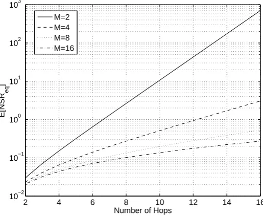
3.2 E[N SReq] for different values of α, N=4, L=4 . . . 48

3.3 Variance of an element of Heq for a M ×M MIMO system . . . 51

3.4 Variance of an element of neq for aM ×M MIMO system . . . 52

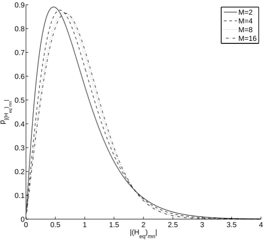
3.5 Probability density function of |(Heq)mn| with N0 = 0 . . . 53

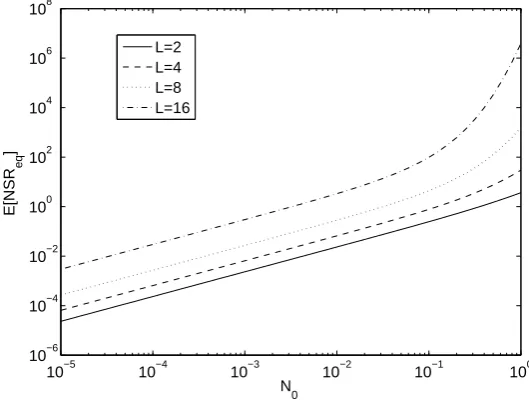
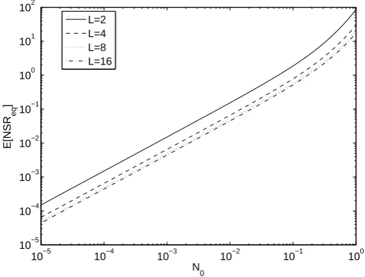
3.6 Plot of expected end to end noise to signal ratios with a SNR of 102 . 54 3.7 Plot of expected end to end noise to signal ratios for a 4×4 MIMO system . . . 55

3.8 Plot of expected end to end noise to signal ratios for a four hop system 56 3.9 Cumulative density of N SReq for a four hop system with a SNR of 10−2 _{. . . 57}

(12)

x

3.10 Cumulative density ofN SReq for a 4×4 MIMO system with a SNR

of 10−2 _{. . . 58}

3.11 Magnitude of the average eigenvalue . . . 58

3.12 Magnitude of the individual eigenvalues for an 8 hop system. . . 59

3.13 PDF of |(Heq)mn|, for a system where H=L= 4 andN0 = 10−2 . . . 59 3.14 PDF of |neq,mn|, for a system where H =L= 4 and N0 = 10−2 . . . . 60

3.15 PDF of |N SReq|, for a system where H =L= 4 and N0 = 10−2 . . . 60

4.1 BER vs the number of hops for stationary AF relay chains at 30dB

SNR. Transmission distance increases with the number of hops. . . . 66

4.2 CDF of SN Req for AF relays in flat Rayleigh fading environments . . 67

4.3 BER vs the number of hops for stationary PF relay chains at 30dB

4.4 CDF of SN Req for PF relays in flat Rayleigh fading environments . . 69

4.5 BER vs the number of hops for stationary DetR relay chains at 30dB

4.6 BER vs SNR for AF relays . . . 71

4.7 BER vs SNR for PF relays . . . 72

4.8 BER vs SNR for DetR relays . . . 73

4.9 BER for PF relays with a fading speed of 100km/h in each link and

no additive noise. . . 74

4.10 BER for DetR relays with a fading speed of 100km/h in each link

and no additive noise. . . 75

4.11 BER vs Doppler Spread for a 4 hop link with PF relays . . . 76

4.12 BER vs Doppler spread for a 4 hop link with DetR relays . . . 77

4.13 2% BER contours for AF relays with 100km/h faded first and last

links. . . 78

4.14 2% BER contours for PF relays with 100km/h faded first and last links. 78

4.15 2% BER contours for DetR relays with 100km/h faded first and last

links. . . 79

(13)

xi

4.17 1% block error rate contours for DetR relays with half rate coding. . 80

4.18 1% block error rate contours for PF relays with half rate coding. . . . 80

4.19 5% block error rate contours for DecR relays with half rate coding. . 81

4.20 5% block error rate contours for DetR relays with half rate coding. . 82

4.21 BER vs SNR for DecR relays with half rate coding. . . 83

(14)

(15)

List of Tables

2.1 Delay spread parameters for radio models, delay in µs and power in

dB . . . 24

2.2 P25 signalling constellation . . . 26

(16)

xiv

Abbreviations

AF - Amplify and forward

BER - Bit error rate

BPSK - Binary phase shift keying

CSI - Channel state information

CB - Citizen Band

DecR - Decode and regenerate

DetR - Detect and regenerate

FIR - Finite impulse response

GEV - Generalised extreme value distribution

ISI - Inter-symbol interference

LOS - Line of sight

MAC - Media access control

MIMO - Multiple input multiple output

SISO - Single input single output

N SReq - Equivalent end to end noise to signal ratio

QAM - Quadrature amplitude modulation

PF - Phase forward

SNR - Signal to noise ratio

SN Req - Equivalent end to end signal to noise ratio

(17)

xv

TCM - Trellis coded modulation

(18)

(19)

Chapter 1 Introduction

When building a communications network, an important consideration is that of

topology [1]. That is, which parts of the network will interact. Two obvious

ar-rangements are centrally routed networks and networks using direct connections.

In a centrally routed network terminal nodes communicate via a single interchange

node. In a network using direct connections terminal nodes communicate directly

with each other. In practice most networks will fall somewhere between these two

extremes. For example, in a cell phone network [2] users communicate via a single

base station within a given area or cell. Users in different cells communicate with

their respective base stations which will transfer the information between them. The

internet works in a similar manner, albeit with a larger hierarchy. Here a user will

connect to an internet service provider, which in turn may connect to a nationwide

exchange and then an intercontinental router. On the other end of the spectrum,

citizen band (CB) radio [3] is an example of a network utilizing direct connections

between users. As may be apparent from the above examples, different topologies

are more appropriate for different types of network.

A centrally routed network is more suited to dealing with a high user density and

can help centralize the cost of establishing a network, that is the capital investment

is primarily in the base stations as opposed to being split evenly between all radio

nodes. In this context, high user density refers to a situation where it can be

expected that a large proportion of the available bandwidth of the network will be

(20)

Chapter 1. Introduction 2

required simultaneously, by a large number of users. This would typically require

bandwidth to be allocated to users dynamically and reassigned with a low latency

[2]. A centrally routed network simplifies this task as, if all communications are

transferred via one node, then the allocation of bandwidth can be managed by this

node alone. This task is referred to as media access control (MAC) [1]. The fact

that MAC can be dealt with solely in the central node allows the majority of the

complexity and therefore the cost of network hardware to reside in this node. The

result of this is the opportunity to produce low cost terminal nodes which, combined

with the centrally routed system’s suitability to high user densities, means that a

network of this style has an easily scalable number of users. In a network with direct

routing all the terminals need to be capable of any MAC the network implements.

This limits the practical user density of a network of this type to the complexity

that can be included in the terminal nodes. As such the investment per user in the

network is higher than a centrally routed scheme but as no additional infrastructure

is required the network can be ad hoc in nature. Systems providing scope for direct

communications between users typically provide more geographical scalability than

centrally routed networks while providing less scope for high user densities. This

is not fundamentally the case but rather arises from the typical implementation of

these network types.

Current radio products are predominantly of two types, privately owned radio

terminals utilizing direct communications on public frequencies and commercial

ra-dio networks [4]. The commercial networks are typically centrally routed, with fixed

high power central nodes. This is the context for the work in this thesis. The key

question is whether some of the flexibility advantages of direct point to point

com-munications can be utilized in radio networks built around expensive fixed base

stations. In particular this work looks at using the concept of relays [5] to provide

this flexibility. A relay in this context is considered to be a network node which

immediately retransmits what it receives, possibly with some intermediary

process-ing. The purpose of the relay node is to extend the range over which other nodes

(21)

nodes to communicate within a given area. It should also remain as transparent as

possible [6]. By transparent we mean that communication between users should be

equivalent to the case where they are in a range where the relay is not needed. That

is the performance and operation of the system should be virtualy the same as in

the case where the relay is not used.

The concept of using relays for communication is not new, in fact it could be

considered as the basis of some of the earliest communication networks. From

semaphore chains to smoke signals to wolf howls, relaying signals provided a simple

means of long distance communication. Modern examples of relays augmenting a

larger network include; relays for cell phone signals located inside large buildings,

which have poor reception from the nearest base station. This relay may be

con-nected to an aerial external to the building, where the signal to the rest of the

network is stronger. A very crude relay is the leaky feeder [7], a length of coaxial

cable which runs along the length of a tunnel and is connected to an aerial

out-side the tunnel. This allows radio signals to propagate inout-side the tunnel. Here we

consider the possibility of a more extensive augmentation of existing networks with

the relay concept, or even stand alone relay based networks. These could be of use

in areas of low user density, where the full sophistication of a base station is not

required. The key requirement of a relay for this purpose is to be of low cost, so as

to provide a useful alternative to installing a base station. Another desirable

prop-erty is to possess a low power requirement. This will allow the possibility of being

battery powered and portable. A product of this nature would provide a low cost,

easily scalable and portable network infrastructure. Situations where this could be

of commercial value include:

• Areas with very low user density, such as rural areas, where little MAC is re-quired. Here the sophistication of a typical base station is unnecessary so a relay

system could provide the same coverage at a much lower cost.

• Temporary networks to provide coverage in remote areas, such as that required

by emergency services. Here the potential portability of relays could be utilized

(22)

be relocated as required.

• Extension of existing networks into areas of low user density. These areas may not prove economic to cover with a base station, but could be serviced by relaying

signals to an existing base station adjacent to the area [8]. This is outlined in

Fig. 1.1.

A

B

Figure 1.1: Coverage for area B with low user density is provided by relaying signals between B and the high density area A

• Extending or establishing new networks in heavily shadowed areas, such as

val-leys, tunnels, buildings etc. Shadowing [9] refers to the situation where large

objects block the path of radio propagation, hills and buildings would be typical

examples. These objects drastically weaken the signal in their path. In areas

with heavy shadowing the use of single high power transmitters is inefficient,

as most of the transmit power is not received. A solution is to use a sequence

of lower power transmitters to relay the signal around the shadowing objects.

Figure 1.2 is an example of this scenario.

Of course an obvious question relating to a relay system of this nature is: how

big can a network based on this concept become? There are two ways to increase

the network coverage, increasing transmit power and adding more relying nodes [5].

Increasing transmit power removes some of the advantages of the relay concept so is

not necessarily desirable. Hence, network expansion would ideally be performed via

(23)

A

B

Figure 1.2: A connection between areas A and B is provided by a relay chain through the shadowing object between them

a signal pass through while retaining an acceptable number of errors. Anyone who

has played the game Chinese whispers will identify the problem that if each relay has

the potential to introduce errors into communication, the combination of multiple

relays increases the probability of errors. To allow the use of chains of relays it is

important to investigate what can be done within the relay node to mitigate this

problem and to establish what kinds of conditions these relay networks can operate

in. This work focuses on the effect of increasing the number of relay nodes in the

communication path, with a variety of relay types and radio environments.

Also under consideration is the use of MIMO transmission with relay networks

[10]. MIMO stands for multiple input multiple output and refers to the use of

antenna arrays for both transmission and reception of information. For example a

single transmitter could use multiple antennas to transmit to a receiver with multiple

antennas. Alternatively a set of transmitters with single antennas could transmit

cooperatively to a set of receivers with single antennas. The advantage of multiple

antennas is that it provides spatial diversity. This effect can provide more reliable

transmission or can be used to increase the potential capacity of a wireless channel.

Due to local scattering effects the strength of a radio signal at separate antennas even

if they are located close to each other can vary drastically. Hence the use of multiple

antennas gives a higher probability of receiving a strong signal at one of the antennas.

(24)

of the channel drops. Furthermore, if the channel properties between each antenna

pair can be tracked by the receiver it is possible to transmit independent information

on each antenna. Antenna arrays at a single node provide this spatial diversity on

a scale of the order of the wavelength of the signal, providing robustness to local

scattering effects. In contrast an array of separate nodes provide a similar effect on a

larger spatial scale. This arrangement can provide redundancy against shadowing as

well as local scattering. The downside to this arrangement is that the geographically

separated nodes need a reliable connection with low delays in order to communicate

cooperatively. This would normally involve a wired connection.

The current knowledge of relay chains can be split into two broad areas:

re-lays using MIMO techniques and those using traditional single antenna systems,

referred to as single input single output (SISO) systems. For MIMO systems, the

results available relating to relay performance are limited but, as with other areas of

MIMO communications, it is an active area of research [11]. Furthermore, multi-hop

relaying using MIMO techniques is in its infancy in terms of performance analysis.

Some results for capacities in relation to numbers of relay nodes and antennas are

available [12, 13]. Optimal relaying techniques and coding structures are developed

in [14] assuming full channel state information (CSI) at each relay. An asymptotic

performance analysis is presented for this system in [14].

Research into SISO communications is more developed, as would be expected

due to its much longer history. It is important to note that these single antenna

systems can still benefit from spatial diversity when multiple relay nodes are used

for signal transmission. As multiple nodes are transmitting the same information in

a multi-hop relay system, a receiver capable of combining signals from all

transmis-sion sources can benefit from this diversity. General results for multi-hop relaying

have still proved difficult to obtain though, an overview of available results is given

in [15]. The system performance is dependent on the type of relay processing

per-formed which complicates a summary of the available knowledge. Introducing the

concepts of analogue and digital relaying make this summary easier. Here, an

(25)

processing, while a digital relay performs some degree of demodulation and

decod-ing before regeneratdecod-ing and retransmittdecod-ing the signal. With an arbitrary hop length

[16] and [17] give upper bounds on errors for digital relays and analogue relays

us-ing a specific amplification factor. [16] contains an analysis for systems usus-ing the

diversity offered by multiple relays and [17] performs a similar analysis for systems

without this diversity. An approximate expression for error rates is developed in

[18] which applies to analogue relays of arbitrary hop length and includes diversity.

The instantaneous end to end SNR is found in [19] for multi-hop analogue relaying

with diversity. The system error rate is found in [20] for digital relays.

1.1 Goals

The available results for multi-hop MIMO relay systems are limited as a result

of the highly complex statistics of the resulting propagation channel. Currently,

the systems are modeled via a combination of the existing models for the channel

between two radio nodes. The result is a model where the degrees of freedom are

proportional to the number of relay nodes and the square of the antenna numbers.

The motivation of the work presented in Chap. 3 is to develop a model which

describes the statistics of the end to end channel directly, ideally massively reducing

the degrees of freedom of the model. This may lead to an easier analysis of the

performance of the system. For example, error rates and end to end signal to

noise ratios for multi-hop MIMO relay channels are not currently available. An

understanding of the statistics of the complete channel may lead to these expressions.

Parallel to this investigation, Chapter 4 looks at performance metrics of a SISO

system using the P25 protocol.

1.2 Contributions

The thesis makes contributions in both areas of interest, namely in the analysis of

MIMO relay channels and in the evaluation of various SISO relay implementations.

(26)

relays. Using this model we go on to develop expressions for moments of the elements

of the end to end transfer function, probability densities for the single relay case

and expressions for the end to end signal to noise ratios in the system. We go on

to look at the effects the relay amplification and a capacity analysis based on the

eigenvalues of the transfer matrix.

The analysis of the SISO system, while providing results for the specific

modula-tion scheme outlined in the P25 specificamodula-tion, also addresses some general quesmodula-tions

arising in the literature. The majority of work done in relation to multi-hop

re-lays focuses on flat fading channels. The SISO simulations presented in Chapter

4 include the error rate trends for multipath channels with a variety of common

relaying protocols. This introduces the problem of inter-symbol interference (ISI),

which proves to be significant and in some cases the dominant cause of errors.

1.3 Thesis Organization

Chapter 2 outlines the existing system models based on single hop transmission and

shows how these can be cascaded to describe a multi-hop system. The description

of the model is split into that relevant to MIMO communications, followed by that

applicable to SISO communications. The description of the system model is further

split into four components, the source signals, the propagation channel, the relaying

protocol and the noise components. These are all described separately for MIMO

and SISO communications.

Chapter 3 develops the statistics of the end to end signal model and presents

the results relevant to performance that can be obtained from this model. A look at

the dependence structure in the end to end transfer function of the channel is given

is presented first, the raw moments of elements of the system model follow. End to

end signal to noise ratio distributions are presented next including their moments.

The effects of the linear amplifiers are considered. The penultimate section contains

an empirical analysis of the eigenvalues with an explanation of how these can be

related to capacity. Finally we look at channel model approximations.

(27)

channel. The simulated results are presented in such a way as to isolate the effects

of individual degrading channel properties. First we demonstrate the effect of slow

fading on the communication scheme across a range of relaying protocols and identify

the cause for the discrepancies in the relay protocols. The results of fast fading are

covered next. Both these sections look at relay protocols ability to mitigate the

effects of frequency selective channels. The complete system model is considered

next. This section looks at conditions in which a desired error rate can be maintained

and is intended to aid system design. The final section looks at requirements for

maintaining block error rates using error correcting codes.

(28)

(29)

Chapter 2 System Model

Transmitter

s₁ r₁

n₁ Channel

H1

Relay 1

Receiver

s_L r_L

Channel HL

n_L

Relay L-1

[image:29.595.142.443.330.486.2]

r_L-1

Figure 2.1: System diagram for a relay chain with L hops

The work in Chaps. 3 and 4 is split into an analytical component involving

MIMO techniques and simulation work based on SISO transmission. As the nature

of many system components is different for these two scenarios, the system model

for each part will be described separately. Given that a SISO communication

sys-tem is a special case of the more general MIMO model, the MIMO section will be

described first in, Sec. 2.3, with the SISO specific model following in Sec. 2.4. As

a preliminary, some notation, performance metrics and system parameters will be

defined. Despite the differences between the two scenarios the common structure of

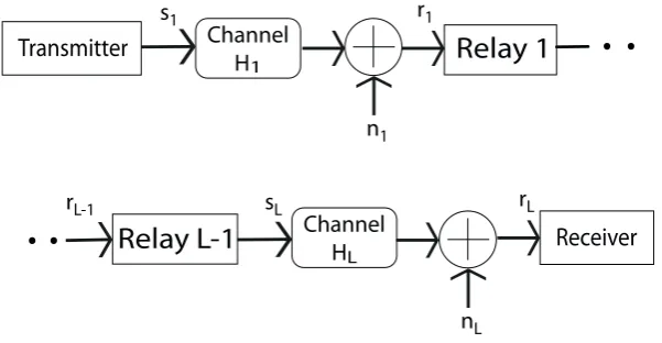
a typical L-hop relay chain can be identified in Fig. 2.1.

To describe the general system in Fig. 2.1 we need to define the signal vectors

s1,s2, . . . ,sL, r1,r2, . . . ,rL and noise vectors n1,n2, . . . ,nL. The originally

(30)

Chapter 2. System Model 12

mitted signal, s1, passes through the first channel, which has transfer function H1. This is received, along with additive Gaussian noise, n1, at the first relay. The received signal, r1, is given as r1 = H1

⊗

s1 +n1, with

⊗

being the convolution

operator. The dimension of the vector s1 is given by the number of transmit an-tennas which in this work will be referred to as N1. The dimension of r1 and n1 is the number of receive antennas, denoted by M1. The received signal, r1, is pro-cessed by the relay, producing the signal transmitted by the first relay, referred to

as s2. The relationship between r1 and s2 depends on the type of relay protocol being employed. r2 is then H2

⊗

s2 +n2 and rL = HL

⊗

sL+nL. The number

of receive antennas at the lth relay and the dimension of the vectors nl and rl is denoted Ml. The number of transmit antennas at thelth relay and the dimension of sl+1 is denotedNl. Given these definitions, the transfer function between thelthand

(l−1)th_{relays has}_N

l−1 inputs andMLoutputs. In general these equations require a

convolution of the signal with the channel transfer function. If this transfer function

is an impulse, then this reduces to a multiplication. In practice, this represents a

channel which does not spread a signal in time. As an approximation to a physical

system this is valid provided the difference in propagation delay across all possible

paths is less than the symbol period. Channels of this type are referred to as flat

fading channels, as the attenuation of the channel is independent of frequency. For

the MIMO system in Chap. 3 a channel model of this form is used. This chapter

looks to provide an expression for the end to end transfer function of the relay link,

that is to specify the signal at the final receiver directly in terms of the originally

transmitted signal. This will be an equation of the form r =Heq

⊗

s1+neq, with Heq being the equivalent transfer function between the transmitted signal and the information carrying component of the received signal. The noise terms, neq,

repre-sents the cumulative noise received through the relay link. It is now left to define

(31)

2.1 Notation

Matrices

• Matrices are represented by bold capital letters such asH.

• Hmn refers to the element from themth row of the nth column of H.

• Hm refers to the mth row of H.

• Hn refers to the nth column ofH.

• Some equations will use specific indices, such as H1, to denote either the

first column or row ofH. Whether this refers to the row or column will be apparent from the context.

• Equations will also use notation such asHl to denote a single matrix from a set of matricesHl, l∈ {1,2, . . . , L}. Once again, the fact that this is a full

matrix rather than a row or column vector will be apparent by context. To

refer to an element of such a matrix the notation (Hl)mnis used to represent

the element from the mth row of the nth column of Hl. Similarly the mth

row ofHl is denoted (Hl)m and nth column, (Hl)n.

Vectors

• Vectors are represented by bold lower case letters such as s.

• sm refers to the mth element of s.

• sk refers to the kth vector in the set sk, k ∈ {1,2, . . . , L}, skm refers to the mth _{element of this vector.}

Products

Empty product expressions are considered to be equal to one. For example,

∏L

l=L+1Hl = 1.

Random Variables

(32)

complex Gaussian variables (ZMCSCG), which are of the form z1 +jz2 where

z1, z2 are i.i.d real zero mean Gaussian variables. We also define CN(0,1) to be

the distribution of a ZMCSCG variable with unit variance.

Complex Variables

Complex conjugates and Hermitian transposes will be denoted by the symbol

†. That is, a scalar x has complex conjugate x†, a vector, s, has Hermitian transposes† and a matrix,H, has Hermitian transpose H†.

2.2 Metrics and System Parameters

When quantifying the performance of communication systems, a variety of metrics

can be used. The metrics used in this work are:

Capacity This is a measure based on information theory giving an upper bound on the rate of the communication system that can be maintained while retaining

no transmission errors.

Bit Error Rate (BER) This metric gives the number of bit discrepancies between the transmitted and received message as a fraction of the total number of bits

contained in the message. The ratio given is normally an average with the

message size tending to infinity as the number of bit errors for any given message

will vary.

Block Error Rate (BLER) Similar to BER the BLER is often applied to trans-mission schemes that send data in discrete, finite blocks. Here the ratio of blocks

containing one or more errors to the total number of blocks transmitted is given.

Fundamentally, all performance measures of a communication system are

depen-dent on the ratio of the received signal power to the received noise power. Let r be

the scalar received signal at a single antenna and n be the scalar noise at the same

single receive antenna. The signal to noise ratio (SNR) is defined as _EE_[[_||_nr|_|22]_] giving

(33)

2.3 Multi-hop MIMO Relayed Communications

Relay Relay Relay

Hk Hk+1

(sk+1)1

(sk+1)M

(rk+1)1

(rk+1)M

(sk)1

(sk)M

(rk)1

[image:33.595.141.440.147.219.2]

(rk)M

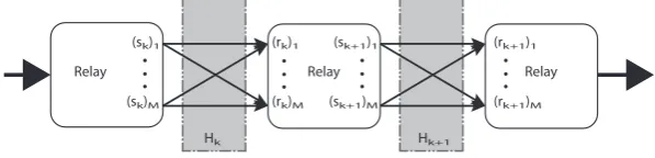
Figure 2.2: System diagram for a partial section of a MIMO multi-hop relay link

For the MIMO system we will focus on flat fading channels. As the transfer

function of this channel is an impulse, the effect of the channel in the system model

reduces to a multiplication. A partial multi-hop MIMO link is shown in Fig. 2.2.

We can define the received signal at the first relay asr1 =H1s1+n1. This received signal is then processed by the relay to give s2, the signal transmitted by the first relay. In general the received signal at the lth _{relay is given by}_r

l=Hlsl+nl.

2.3.1 Channel Model

For the MIMO relays the standard Rayleigh scattering model of wireless propagation

is used. Here the gain between any transmit/receive antenna pair is given by a

variable distributed as a ZMCSCG variable. The model represents propagation

scenarios in which there is no line of sight (LOS) path present and it assumes a

large degree of scattering of the signal at the receiver. It can be shown in this

situation that the attenuation between an antenna pair is Rayleigh distributed [9].

Hence the PDF of the channel attenuation is given in [21] Chap. 18 Sec. 10.2 as

p(x) = x

σ2 exp

(

−x2

2σ2

)

, x≥0

whereσ is the distribution scale parameter, which in this case specifies the average

channel attenuation. The phase shift of the channel is uniformly distributed between

−π and π.

In a MIMO system [22] the gains between each antenna pair can be represented

(34)

H=

    

H1,1 · · · H1,N

..

. . .. ...

HM,1 · · · HM,N

    ,

for a MIMO system with N transmit antennas and M receive antennas. Such a

system will be referred to as M×N MIMO. Each element, Hm,n, inHis distributed as an i.i.d ZMCSCG variable. His referred to as the channel matrix. Ifsis anN×1 vector representing the signals at the N transmitters then the signals received at the

M receivers are given as r=Hs. In the presence of noise this becomes r=Hs+n

where n is an M ×1 vector of i.i.d complex Gaussian variables.

The Rayleigh model represents local scattering of the signal at the receiver. To

account for shadowing between transmit and receive antennas an additional

log-normal scaling parameter is log-normally used, while free space path loss is represented

by another parameter. The work in Chaps. 3 and 4 does not focus on a specific

physical system so a distance or antenna coefficient for the free space path loss

cannot be specified. Shadowing is also a constant scaling parameter for a given

inter node channel. Hence we remove both of these components from our channel

model and instead we simply specify the SNR at the receiver. This is justified based

on the fact that for a physical radio link the degree of shadowing experienced will

remain relatively constant over the period of transmission. Hence from the point

of view of system design it is just as useful to evaluate the links performance at a

given average SNR.

Time Varying Channels

The channel model described here is based on the idea of a large number of scattered

signal paths combining randomly at the receiver to produce the received signal. This

suggests that the received signal will vary in space. Hence a moving receiver will

experience a time dependent channel. Similarly, if an object around the receiver

that is affecting the scattered signal is moving, then even a stationary receiver

will experience a channel that varies over time [9]. The effect is the same if the

(35)

and objects in the propagation environment dictates the extent of this effect. For

the purpose of analysis in wireless communications, the rate of change of the channel

is broken into two categories, these being fast and slow fading channels. In a slow

fading channel the rate of change of the channel is considered to be of an order such

that over a symbol period of the modulation scheme the channel can be considered

to be static. In this situation the performance of the communication scheme is not

affected directly by the changing channel, but the average performance of the system

will be dependent on how the channel properties change over time. In a fast fading

environment the channel properties are assumed to change significantly within a

symbol period and will potentially affect the demodulated signal.

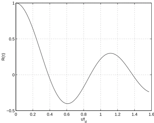
We use a model of fast fading based on the Jakes Doppler spectrum [9]. With

this model the change over time can be defined by an autocorrelation function

R(τ) =J0(2πfdτ) whereJ0 is the zeroth-order Bessel function of the first kind,fd is

the maximum doppler shift andτ is the time between two channel instances. R(τ) is

the autocorrelation function of an element of the channel matrix,H. For the complex element,Hmn, the autocorrelation function is defined asR(τ) =E[(Hmn)†t(Hmn)t+τ],

where the subscript refers to the time at which Hmn is observed. The maximum

doppler shift is defined as fd = vf_cc where fc is the carrier frequency and v is the

relative velocity of the transmitter and receiver or the scattering objects. Figure

2.3 is a plot of the normalized auto correlation and gives a measure of the expected

commonality between two instances of the channel with a separation in time given

by _fτ d.

The effect of a time varying channel on the received signal depends on the type

of modulation employed by the communication system. When using a constant

envelope, non-coherent modulation such as DPSK the change in channel properties

across adjacent symbols introduces errors in the received signal. When designing a

system to operate in these conditions the autocorrelation function of the channel can

be used to give an indication of acceptable symbol rates for a given error margin.

It can be seen from Fig. 2.3 that the higher the symbol frequency the greater

(36)

0 0.2 0.4 0.6 0.8 1 1.2 1.4 1.6

−0.5 0 0.5 1

τ/f_d

R(

τ

[image:36.595.151.413.110.318.2]

)

Figure 2.3: Fast fading autocorrelation function

modulation a change in the channel phase shift between sample times will introduce

an error in the demodulated signal. Hence, a higher correlation between channel

properties at adjacent sample times results in a lower error probability. Figure 2.3

also suggests that there is a lower limit to symbol frequency for a practical DPSK

system giving by the first zero crossing of the channel autocorrelation function.

At this point the channel properties are not reliably correlated between adjacent

samples.

2.3.2 Source Signals

The source signals, s1, are N1×1 vectors drawn from a random sequence at a rate given by the sample frequency of the communication protocol. The samples drawn

from the sequence are assumed to be uncorrelated. Furthermore E[s†₁s1] is assumed to be equal to one.

2.3.3 Relay Protocols

The types of relaying considered are split into two general categories. In the

(37)

correspond to the use of analogue or digital relays respectively. In decoded relaying

the message is estimated at each relay and regenerated. As a result, the end to end

channel properties are not important and each hop in the relay link can be

con-sidered independently. The problem in evaluating the performance with decoded

relaying becomes one of describing error propagation as decision errors from one

relay will be transmitted to the next. Chapter 3 does not look at this issue and

the analytical work focuses on linear relaying. Relays of this type retransmit the

received signal with some form of linear transformation, α, hence the transmitted

signal for relay one is given bys2 =α1r1 where

s2 =α1(H1s1+n1).

This pattern can be continued to give the signals throughout the relay chain.

Let the received signal at thelth relay berl, the signal transmitted from thelthrelay besl+1, the channel transfer function between the (l−1)th and lth relays be Hl and

the received noise at the lth relay be nl. With these definitions

rl =Hlsl+nl,

sl+1 =αlrl,

sl+1 =αl(Hlsl+nl). (2.1)

Expanding (2.1) recursively we can define the signal at the final receiver, rL,

in terms of the signal at the original transmitter, s1, giving an end to end system equation. This is shown in Sec. 3.1.

The general form forαl is anMl×Nl complex matrix. This allows the possibility

of the output at each antenna on the transmit side of the relay being a linear

combination of the inputs at each antenna on the receive side. An important special

case of this general form is a diagonal αl matrix. Here, the signal received at each

antenna is scaled to give the output at a transmit antenna. Hence there is no

combining of signals, simply a scaling. A further simplification is the reduction of

αl to a scalar, where there is once again no combining of signals and only a simple

(38)

2.3.4 Noise

The system model includes additive Gaussian noise at each receive antenna.

Com-plex Gaussian noise is assumed. Hence the noise, n, is given by

√

N0

2 (nr+jni) where

nr and ni are i.i.d real Gaussian variables andN0/2 is the power spectral density of the noise.

2.3.5 Signal Power

To provide a general model for the relay system it is desirable to normalize the

signal powers in the system model. To achieve this the various parts of the system

can be redefined as follows. Let the physical signal at the first relay be defined by

˜s2 = ˜α( ˜H1˜s1+ ˜n1). (2.2)

We will write (2.2) in terms of a set of signals with unit power scaled by the

power of the signals in the actual physical system.

√

Ps2s2 = ˜α(

√

PHH1

√

Ps1s1+

√

Pnnˆ1) (2.3)

Here, H1 is the normalized channel matrix where E[|(H1)mn|2] = 1, s1, s2 and ˆn1 are normalized transmit signals and noise vectors in the same fashion.

Ps2 = E[˜s

†

2˜s2], Ps1 = E[˜s

†

1˜s1], PH = E[|( ˜H1)mn|2], Pn = E[|n˜1,m|2]. Dividing (2.3)

by √PHPs1 we have

√

Ps2

√

PHPs1

s2 = ˜α(H1s1+

√

Pn

√

PHPs1

ˆ

n1),

s2 =

√

PHPs1

√

Ps2

˜

α(H1s1+

√

Pn

√

PHPs1

ˆ

n1).

If we then define a normalized amplification factor, α, as

α=

√

PHPs1

√

Ps2

˜

α,

(39)

E[n1n†1] =

Pn PHPs1

I,

then we have the normalized system model

s2 =α(H1s1+n1).

Since α is still an arbitrary scaling variable we can represent the various signal

powers in the system by the variance of n1 alone. Furthermore, _PPn

HPs₁ is equal to the inverse of the signal to noise ratio, _{SN R}1 , and the model can be defined directly by this parameter. Hence in system modeling it is sufficient to define the SNR and

use unit power channels and signals.

2.4 Multi-hop SISO Relayed Communications

When using SISO communications the system model becomes scalar, but here we

allow the possibility of the radio channel spreading the signal in time. This requires

a convolution in the system equations. The received signal at the first relay, r1, is

given byh1

⊗

s1+n1. In SISO systems the possibility of non linear relay processing

is considered, so an end to end system equation is not necessarily obtainable. The

signals at thelth_{relay can still be defined as}_r

l,sl+1andnlwith the transfer function

between the lth _{and (}_l₋₁₎th _{relay being} _h

l. The received signals are defined by

rl=hl

⊗

sl+nl.

The relationship between rl and sl+1 depends on the relay protocol employed and is covered in Sec. 2.4.5.

2.4.1 Channel Model

Here we use the flat Rayleigh channel as a reference to which the more complex

propagation models can be compared. In the results presented, the flat Rayleigh

(40)

the other channel distortions to be assessed by comparison. The other channel

mod-els used here are extensions of the Rayleigh propagation concept, which allow the

inclusion of phenomena such as ISI and the time varying channel causing distortion

of the demodulated signal. These extended models will be described here.

While the Rayleigh model accounts for the local scattering of the received signal

it does not allow for a LOS signal from the transmitter. The model can be extended

to allow a non zero mean amplitude representing the presence of a LOS path. This

is referred to as a Rician channel [9], where the channel attenuation distribution is

defined by the PDF [21] Chap. 18 Sec. 10.7

p(x) = x

σ2 exp

(

−(x2₊_µ2₎ 2σ2

)

I0

(_xµ

σ2

)

, x≥0 (2.4)

and I0(x) is the first order Bessel function of the second kind. In (2.4), µ is a

location parameter and represents the attenuation of the LOS path, while σ2 _{is a}

scale parameter. The average channel attenuation is given by 2σ2₊_µ2_{. The phase}

shift is once again uniformly distributed between −π and π.

Relay zN1

st+N1

z-1

st-1

n s

Relay r

H

z-N2

st-N2

Figure 2.4: Multi-path channel model

The Rician/Rayleigh model accounts for local scattering of the signal at the

receiver but, as the possible phase shift is limited to the range [−π, π), it does not

include the effects of ISI. More complex propagation models can account for received

signals with varying amounts of delay by including additional paths with delayed

versions of the transmitted signal. This model can now reproduce the effects of

(41)

symbols. The properties of a variety of radio environments can be represented

using combinations of path delays and expected attenuations. If the individual

path gains are considered to be uncorrelated, the baseband signal can be described

mathematically using a finite impulse response (FIR) structure

rt= N2

∑

n=−N1

hnexp(θn)st−n,

where hn and exp(θn) make up the complex weights of the FIR filter. Details of

how the weights are obtained are given in Sec. (4.2).

2.4.2 Radio Environments

The environment models used are taken from [23]. These specify power delay

pro-files based on measured data in a set of European locations designed to replicate

the nature of propagation in general locations of a similar nature. The

environ-ments modeled are rural, urban, hilly rural and hilly urban scenarios. As a point of

reference, a flat Rayleigh environment has also been simulated. The environment

models are defined in Table 2.1. In the simulations the expected channel gains are

normalized to unity. The models define a delay and a gain for each path with the

shortest path assigned a delay of 0s and the strongest path a gain of 0dB. The

sam-ple period of the modulated signal is 21µs. The rural environment is the simplest

radio environment with a small delay spread and half the signal power existing in

a line of sight (LOS) path. This is representative of a high site situation where

the relay nodes could be located on adjacent hilltops for example. The hilly rural

environment has no LOS path and a much larger delay spread, 17µs at -12dB as

opposed to 0.5µs at -20dB. This is representative of a situation such as a series

of relays placed along the length of a valley. The urban environment includes a

longest delay of 5µs at -10dB and the strongest path delayed by 0.2µs. The hilly

urban environment has a sightly longer maximum delay of 6.6µs with the signal

power more evenly distributed across the delay spread. It is important to consider

a range of radio environments as different systems may be better suited to different

(42)

Table 2.1: Delay spread parameters for radio models, delay in µsand power in dB

Tap Rural Urban Hilly Urban Hilly Rural

Delay Power Delay Power Delay Power Delay Power

1 0 0 0 -3 0 -3 0 0

2 0.1 -4 0.2 0 0.4 0 0.2 -2

3 0.2 -8 0.6 -2 1.0 -3 0.4 -4

4 0.3 -12 1.6 -6 1.6 -5 0.6 -7

5 0.4 -16 2.4 -8 5.0 -2 15 -6

6 0.5 -20 5.0 -10 6.6 -4 17.2 -12

Considering the effect of multiple relay nodes on the end to end radio channel

makes the propagation channel much more complex. To get a feel for the resulting

channel, consider a SISO system with linear relays in the absence of noise. Starting

with the flat Rayleigh case, when a set of these channels are combined in series the

output becomes

rt=

∏

n hnst.

If we define the channel gain, hn, in polar form, that is hn = Anexp(jθn), the

total phase change of the channel becomes ∑_nθn. The combined amplitude is

∏

nAn. Since

∑

nθn is the sum of N circularly symmetric, independent, uniformly

distributed random variables it is also distributed uniformly in the interval [−π, π).

The combined amplitude is distributed as a product of Rayleigh variables.

Next we consider the multi-path channel model where

rt= N2

∑

n=−N1

hnexp(θn)st−n.

The combination of these channels becomes more cumbersome to describe

math-ematically. To circumvent this, first we define ϕd as a shift operator such that ϕd(st) =st−dandϕd1(s)ϕd2(s) = ϕd1+d2(s). With this notation, the output can then

be given as

rt= L

∏

k=1

[ _N

2

∑

n=−N1

hnexp(θn)ϕdkn(st)

]

.

(43)

the original paths. Considering one of these path combinations, the amplitude is

again distributed as a product of Rayleigh variables and the phase is uniform on

the interval [−π, π). Finally, the delay is the sum of the delays of the individual

paths that make up the end to end paths. To assess the nature of the end to end

channel it is useful to consider the power delay profile. That is the expected signal

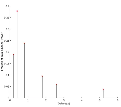
power at the receiver over time corresponding to an instance of a transmitted signal.

For example, the power delay profile of the urban channel as defined in Table 2.1 is

given in Fig. 2.5.

0 1 2 3 4 5 6

0 0.05 0.1 0.15 0.2 0.25 0.3 0.35 0.4

Delay (µs)

[image:43.595.160.419.286.515.2]

Fraction of Total Channel Power

Figure 2.5: Power delay profile for urban environment

As these profiles define the transfer function of the channel the profile for

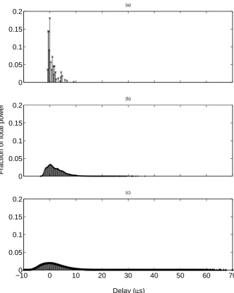
multi-hop channels can be obtained by the convolution of the transfer functions. Figure

2.6 shows how the distribution of signal power in time is affected by multiple relay

nodes.

As the number of hops increases, the dispersion of the signal in time increases.

Without a receiver with the ability to equalize the channel, not only will the received

power decrease as the transmitted power is spread outside the sample period, but

this proportion of the transmitted power will also interfere with adjacent symbols.

(44)

sample time at the receiver will not necessarily be aligned with the peak received

power.

2.4.3 P25 Communications

We give special attention in this work to the P25 communication protocol. This

uses a non-coherent frequency/differential phase modulation. The protocol maps 2

bits per symbol. While the P25 specification [24] allows some variation in the details

of implementation, our system uses differential phase shift modulation. Here, the

signal is represented by the change in phase between successive sample periods. The

message bits are grey coded to symbols as given by the signal constellation in Table

2.2. The signal to be transmitted, s, is given by

Table 2.2: P25 signalling constellation Bits Phase Change

10 -135

00 -45

01 45

11 135

st=st−1exp(iθt),

where the subscript t gives the sample time and θ is the message symbol.

P25 communications have several advantages for wireless propagation. The

con-stant envelope frequency/differential phase modulation is not susceptible to

distor-tion due to a constant complex gain in the propagadistor-tion path. Though the

demodu-lated signal is affected by a time varying phase change in the propagation path, the

extent of this effect is proportional to the rate of change of the channel phase and

the symbol rate chosen for modulation. The protocol, being non-coherent and not

taking advantage of any channel state information, will not provide a high

band-width efficiency in challenging propagation environments. The payoff for this is low

complexity radio hardware.

The symbol frequency is 4.8kHz, the modulation frequency 48kHz. The

(45)

offers a higher level of robustness in fast fading channels. Conversely, the symbol

frequency is lower than the modulation frequency, as this reduces susceptibility to

ISI. The carrier frequency is 800MHz. To demodulate the received signal, the phase

difference between successive samples is calculated and the result mapped back to

the appropriate bits.

The receiver works as follows. The phase change between samples, ˆθ, is obtained

as,

ˆ

θ =arg(rtr†t−1). (2.5)

This phase change is then mapped to the closest valid symbol, that is the value of

m′ ∈ {−3,−1,1,3} that minimizes

arg

(

ritr_i∗₍_t₋₁₎exp

(

−jπm′

4

)) .

The protocol also specifies a forward error correcting (FEC) scheme based on a

convolution code. The code is based on a 96 symbol block and has a 1₂ data rate. The

symbols to be transmitted are interleaved before passing through the convolutional

encoder and modulated as above. At the decoder, demodulation is performed as

normal then a Viterbi decoder is used to estimate the interleaved symbols. These

are then deinterleaved to recover the original symbol sequence.

2.4.4 Noise

The system is modeled using complex Gaussian noise. This is of the same form as

used in the MIMO model. Hence the noise, n, is given by

√

N0

2 (nr +jni), where

nr and ni are i.i.d real zero mean Gaussian variables and N0 is the average noise power.

2.4.5 Relaying Protocol

The primary requirements of the relays are for them to be of low cost and power.

This is the advantage it offers over a centrally routed (ie. base station) network.

(46)

maintaining a reasonable capacity over the link is also a requirement and this can

become challenging as the number of relay nodes increase. To produce a practical

communication system, the relay nodes must control the cumulative negative effects

of the multi-hop propagation environment.

The simplest form of relay is a fixed gain amplifying relay in which sl+1 =αlrl,

where αl is a constant scalar. In this type of system, the amplification factor, αl,

can be designed to control the expected transmit power, E[|sl+1|2]. To maintain a constant value for E[|sl|2], l ∈ 1,2, . . . , L, the amplification factor can be set as

αl =

√

1

E[|hl|2]+N0. This scheme will require expensive linear amplifiers. It also

will prove unstable for channels with a large variance as there is no control over

the instantaneous transmit powers, s2

l+1. The scheme requires knowledge of the expected channel attenuations, E[|hl|2], and expected noise power at the receiver, N0.

If the relay is capable of tracking channel state information, a better system

would use an adaptive gain, where αl =

√

1

|hl|2+N0. A special case of this scheme

can be applied to constant envelope modulation schemes. If no information is carried

in the amplitude, the relay node can simply take the phase of the received signal

and retransmit this at the desired power. Mathematically, this is equivalent to an

amplification factor, αl =

√

1

|rl|2, and requires no knowledge of the channel state or received noise power. The fact the transmission power can be controlled precisely

means the maximum power of information carrying signal can be transmitted at any

given instance. Constant transmit power also allows the use of simple and cheap

non-linear amplifiers.

Looking at decoding relays, the simplest relaying protocol detects message

sym-bols then regenerates the estimated signal for transmission. This protocol requires a

digital relay. In these relays the signal is shifted from pass band to base band and a

differential detector is used to estimate the transmitted message symbols as per the

P25 protocol. Differential modulation is then used to produce the signal imposed

on the carrier signal for transmission. This also allows the transmit power to be

(47)

the information carrying signal power and allowing the use of simple, non-linear

amplifiers. There are other significant advantages to the decoding and

regenera-tion of the message at each relay. It removes the effects of the multi-hop channel,

only suffering from the results of channel distortion between each relay pair. The

downside of this scheme is that any decoding errors at the relays will be propagated

through to the final receiver.

The simulation work undertaken investigates four options for relaying protocols.

These are referred to as Amplify and Forward (AF) [25], Phase Forwarding (PF),

Detect and Regenerate (DetR) [26] and Decode and Regenerate (DecR). The AF

protocol use the fixed amplification scheme giving a constant expected transmit

power across all the relay nodes. PF relays use the phase only transmission scheme,

providing constant power transmission. The DetR protocol is the basic digital relay,

demodulating the input signal to perform symbol estimation before regenerating the

signal for transmission. This protocol also allows constant power transmission. The

DecR protocol is based on the trellis coded modulation (TCM) scheme of the P25

specification. In this case the relay nodes perform symbol detection in the same way

as for DetR. Then, the most likely transmitted data sequence is estimated from the

received symbols using a Viterbi algorithm. This estimate of the transmitted signal

(48)

0 0.05 0.1 0.15 0.2

(a)

0 0.05 0.1 0.15 0.2

(b)

Fraction of total power

−100 0 10 20 30 40 50 60 70

0.05 0.1 0.15 0.2

(c)

[image:48.595.113.445.200.616.2]

Delay (µs)

(49)

Chapter 3 Statistical Properties of Multi-hop

Relay Chains

This analysis of relay chains focuses on the use of linear relays in flat Rayleigh

radio environments. The flat Rayleigh model is used as this is the most important

baseline case and leads to a multiplicative channel model, as opposed to requiring

a convolution operation which results from the use of a multi-path model. As the

statistics of the flat Rayleigh case are already highly complex, the multi-path case

has been left to be considered in future work. Detect and regenerate relays are

also not considered in this section. The reason for this is that in decoding relays

the message is regenerated at each relay and so the problem becomes one of error

propagation and the propagation channel between each relay pair can be handled

independently. To recap the system model presented in Sec. 2.3, the communication

system is represented at the lth relay by

sl+1 =αlrl

=αl(Hlsl+nl).

In Secs. 3.3-3.5 the linear amplification term,α, is left arbitrary. To give explicit

results in these sections we assume that it is a constant.

The focus of this section is the development of an end to end system model, of

the formrL=Heqs1+neq. Ideally this will prove useful in analysis of properties such as end to end capacity and BER. An end to end model is found for a multiple input

(50)

Chapter 3. Statistical Properties of Multi-hop Relay Chains 32

single output (MISO) system. We use this to characterise end to end properties

including noise to signal ratios and the moments of elements of the channel matrix

and noise vector. Additionally, the dependence structure in the end to end model

is established for MIMO systems. Finally, a characterisation of the eigenvalues of a

MIMO system is presented.

3.1 Equivalent Channel Matrices

Transmitter Relay

Receiver

H1 h2

s2,1

s2,2

r2

s1,1

s1,2

r1,1

r1,2

Figure 3.1: Example of a simple MISO system

Here we construct an end to end model for a MISO system. This can also be

applied to a MIMO system to give properties relating to a single receive antenna.

Consider a MISO system in the context of a relay chain. Here, arrays of antennas at

the source and relays transmit to arrays of receive antennas, with the constraint that

the final receiver has only one antenna. This reduces the channel matrix between

the final relay and receiver to a vector. We will look at a specific case of this type

of system to illustrate the method of obtaining the equivalent model. Consider a

system using a 2×2 MIMO link followed by a single antenna receiver, as in Fig.

3.1, with a flat Rayleigh channel and linear relaying. For this example we have the

channel model,

r2 =

[

h2,1 h2,2

]

α1

  

(H1)1,1 (H1)1,2 (H1)2,1 (H1)2,2

 

 s1,1

s1,2

 +

 n1,1

n1,2

 



+n2. (3.1)

Analysis of MIMO Relay Chains