Diagram methods for reduction factor calculations in Jahn Teller systems

DIAGRAM METHODS FOR REDUCTI ON FACTOR

CALCULATIONS IN JAHN-TELLER SYSTEMS

A thesis

submitted in partial fulfilment

of the requirements for the Degree

of

Doctor of Philosophy

in the

University of Canterbury

Christchurch, New Zealand.

by

S. H. r:ayne

,-;:,-,"

University of Canterbury

SCIENCES LIBRARY

ABSTRACT

A novel method is developed for the description and calculation of

Ham reduction factors in 'Jahn-Teller active' systems which are weakly

coupled to many lattice modes. Diagrammatic many-body perturbation theory

for finite temperatures is combined with diagrammatic group theory into a

coherent formalism, whose essential features are readily visualized. The

method lends itself to economical calculation of reduction factors (given

the recent availability of 6j symbols for crystal point group) and also to

generalization of the traditional single multiplet 'Jahn-Teller problem' •

Multirnode effects may be distinguished experimentally by searching for

particular combinations of reduction factors, associated with particular

Feynman diagrams, that vanish to all orders in systems with a continuous

symmetry group and to fourth order in all , within a single-mode

coupling model.

octahedral

General expressions for reduction factors are derived for

up to at least fourth order, and including lattice

anhar-monicity and non-linear electron-phonon coupling. The effects of symmetric

vibrations and intermultiplet coupling on reduction factors, and

CONTENTS

INTRODUCTION

CHAPTER

I

I I

III

VIBRONIC REDUCTION FACTORS

1. CONSTRUCTION OF EIGENSTATES

2. REDUCTION FACTORS

3. JAHN-TELLER SYSTEMS IN OCTAHEDRAL SYMMETRY

3.1 Doublet states -

r

3 3.2 Triplet states

- r

5 3.3 _{Quartet states - f8}

4. EXTENDED MULTIPLETS

5. SUMMARY

REDUCTION FACTORS VIA GREEN FUNCTIONS

1. A PERTURBATIVE SOLUTION FOR THE ION-PHONON SYSTEM

1.1 The Green function formalism

1.2 Comparison with standard procedure

2. AN EFFECTIVE EXTERNAL PERTURBATION

3. FEYNMAN TO GROUP-THEORETIC DIAGRAMS

4. 'ELECTRONIC' REDUCTION FACTORS

5. SUMMARY

JAHN-TELLER SYSTEMS IN OCTAHEDRAL SYMMETRY - I

1. METHOD OF CALCULATION

2. LINEAR ION-PHONON INTERACTION - f3 x E 2.1 Reduction factors to fourth order

2.2 Generalizations to higher orders

PAGE

1

4

4

7

12

13

13

15

20

21

22

22

22

30

32

36

39

44

46

46

51

51

54

3. GROUP-THEORETIC STRUCTURES OF ALL FEYNMAN DIAGRAMS 58

3.1 Arbitrary symmetry

3.2 Application to f 3 X. E

58

IV

4. LINEAR, NON-LINEAR, ANHARMONIC INTERACTIONS

4.1

4.2

5. SYMMARY AND DISCUSSION

JAHN-TELLER SYSTEMS IN OCTAHEDRAL SYMMETRY - II

1. TRIPLET STATES - f5 x €

67

67

75

SO

83

S3

1.1 Linear interaction - an exact solution

S4

1.2 Inclusion of non-linear, anharmonic couplings 87

2. TRIPLET STATES - OFF DIAGONAL INTERACTIONS

2.1 Linear interaction

2.1(a) x 1:2

2.1(b) x (

2.1(c) Equal coupling - f5 x (£=1: 2)

90

90

91

92

94

2.2 Linear, non-linear, anharmonic interactions - 95

f 5 x 2)

3. QUARTET STATES

3.1 Linear interaction

3.1(a) fS x €

3.1(b) fS x 1:2

3.1(c) fS x (£+1: 2)

3.1(d) Equal coupling - fS x (£=1: 2)

97

97

97

98

100

105

3.2 Linear, non-linear, anharmonic interactions - 105

f S x (a

l +£+1:2)

4. DISCUSSION

4.1

4.2

4.3

Features of the f

5, fS systems Other lattice models

Predictions for any symmetry

5. OTHER ASPECTS OF THE FORMALISM

5.1 Intermultiplet coupling

5.2 Higher-order reduction factors

lOS

lOS

110

113

119

119

124

APPENDIX

I

II

III

IV

V

VI

VII

REFERENCES

PUBLICATIONS

TABLES OF j SYMBOLS FOR THE OCTAHEDRAL GROUP, 0

LABELLING OF THE VIBRATIONAL STATES FOR THE

JAHN-TELLER SYSTEMS,

-/r

8 x

(E=L

2)

MULTIPLICITY CONSIDERATIONS FOR THE

r8

STATES

j SYMBOLS FOR THE GROUP S05

REDUCTION OF GROUP-THEORETIC STRUCTURES TO j SYMBOLS

METHODS FOR EVALUATING FEYNMAN DIAGRAMS AND LATTICE SUMS

ELIMINATION OF THE LINEAR INTERACTION TRANSFORMING AS

r

1

ACKNOWLEDGEMENTS

PAGE

130

137

139

142

144

149

155

158

162

FIGURE PAGE

1 10

2 25

3 27

4 34

5 37

6 41

7 48

8 56

9 59

10 61,62

11 66

12 69,70

13 77

14 89

15 101

1.

INTRODUCTION

When the coupling of an impurity ion to a host crystal lattice is

not so strong, that the Jahn-Teller instability of degenerate electronic

states lowers the site symmetry of the ion, the system is said to exhibit

the dynamic Jahn-Teller effect (DJTE), (Ham (1972), Englman (1972».

The coupling between the lattice vibrations and the electronic states now

modifies the energy levels of the combined (vibronic) system in a non-trivial

manner, even for weak coupling. Ham first recognized the import of the

DJTE for the interpretation of EPR and optical spectra of impurities: when

a symmetry lowering perturbation is applied to the ionic levels, i t is the

vibronic, and not the electronic states, which determine the response.

He introduced the concept of reduction factors (RFs) to describe the (observed)

reduction of electronic matrix elements of the perturbation, as a result of

the vibronic coupling. Since the magnitudes of the RFs contain details of

the ion-lattice interaction, their measurement, and the theoretical models

advanced for their ion, have played important roles in the

under-standing of impurity-host It is these models that are our concern.

Ham's (1965, 1968) initial model for RFs, was based on the coupling

of the ion to the linear ( ) displacements of the nearest neighbours,

assuming a single frequency for this vibration. For example, for the case

of an electronic doublet in cubic ,

r

3, coupled to a

r

3-typ e vibration,

r3

x E, the vibronic ground states related the two RFs, p,q for this system, as q = ~ (l+p) . This simple model was used with reasonable success, and held sway until 1973, when Englman and Halperin and, simultaneously, Gauthier

and Walker, showed the above relation to be incorrect when the coupling was

to more than one mode fre~uency. imental confirmation of their

pre-diction followed (Abou-Ghantous et al. (1974». Bates and co-workers

(Bates (1978) - this article reviews theoretical treatments) have also

developed a multimode coupling model for some Jahn-Teller (JT) systems.

The methods of calculating RFs, used by the above authors and others, can be

divided into three categories:

(i) Construction of the eigenstates of the vibronic Hamiltonian (e.g.

Ham, Halperin and Englman) - the standard method. It lends itself

to a determination of the relations between RFs that can follow from

(ii) Transformation of the vibronic Hamiltonian and external perturbation

(Bates) - applicable for linear ion-lattice coupling of JT ions in

certain symmetries (it is only exact for one system).

(iii) Green function methods (Gauthier and Walker) - valid for weak coupling.

Though each of the three methods has its limitations, the first is inferior

to the other two, because the dependence of the RFs on temperature, and on

the coupling of the ion to the continuum of lattice modes, cannot be easily

calculated. However, despite the work of the above authors and others,

several important problems remain outstanding: a unified approach to RF

cal-culations for JT systems of any symmetry, has yet to be given; the coupling

of the ion to the lattice has usually been considered in some restricted form;

temperature effects, in combination with the continuum coupling, have not

been examined carefully; nor has there been a general formulation to allow

the treatment of other considerations, such as coupling between separated

electronic states and higher order RFs. With the restriction to a weak

coupling solution, we redress this situation. We follow Gauthier and Walker's

initiative, and use the thermal Green function method. This borrows the

techniques of quantum field theory: perturbative expansions in any interaction

are conveniently represented as Feynman graphs. Relevant physical quantities

can then be calculated to desired orders, by summing the appropriate graphs.

In our case though, these graphs are not merely useful visual aids. Unlike

Gauthier and Walker, we represent

all

algebraic aspects of the formalism by

diagrams, as the details of the symmetry constraints on the ion-lattice and

the perturbing interactions are latent in these diagrams, and can be extracted

with the aid of Stedman's (1975, 1976) diagram technique for groups. We

use this technique to maximum advantage to reduce computations. The result

is a systematic, and novel, method for the calculation of RFs for any JT

system.

In Chapter I, we give the most general formulation of RFs that follows

from a knowledge of the symmetry of the system eigenstates alone. Previous

treatments are insufficient for our purposes. Relations between RFs for

multiplets in octahedral symmetry, the systems of later interest, are

calcul-ated. The Green function formalism is presented in Chapter II, our diagram

method developed, and RFs defined in an analogous manner to that in Chapter I.

In Chapter III, we derive analytic expressions for the RFs for the electronic

doublet,

r

as functions of coupling type, lattice frequencies, and temper-3,

3.

This analysis is extended to the more complicated octahedral systems in

Chapter IV. For all systems, we examine the implications of our formulae

for the interpretation of RFs. Comparisons with previous theoretical

treatments are made throughout. Appendices of tables and diagrams are

included so that our calculations may be followed.

As additional examinable material, we present at the end of the above

work, a paper which considers some consequences of ion-lattice coupling for 2+

CHAPTER I

FACTORS

We give a general group-theoretic construction for the

of the vibronic Hamiltonian. Following a generalization of Ham's definition

of reduction factors i t is shown how to extract the symmetry information in

them with a knowledge of the j symbols of the invariance group of the Hamil-tonian. We introduce the diagram method for groups for this. We then

determine the relations between reduction factors for isolated multiples in

cubic symmetry and review the work which has been done in this area. Lastly

we remark on systems that have a more complicated energy level structure.

1. CONSTRUCTION OF EIGENSTATES

We shall describe the electronic energy level scheme of an impurity ion

in the perfect host crystal by the eigenvalue equation,

He ~ (q) ~ E ~ (q)

a a a

where q represents the electronic coordinates.

electronic Hamiltonian, H , is not of interest e

terms (free iOn, static crystal field,

(I-I)

The form of the

, but i t will contain all

etc.) which are larger in

magnitude than the dynamic interaction between the ion and the lattice .

The complete set of eigenfunctions {~ } will then form a good basis for a a

linear vector space V (a subspace of Hilbert space).

q The energy levels of

the host lattice vibrations (phonons) can be described similarly - a

Hamil-tonian Hp with eigenfunctions

Xa(Q) (Q

the vibrational coordinates) spanning

a vector space V

Q

.

The vibronic Hamiltonian for the interacting electron-phonon system is

written as

H H

+

H

+

V(qQ)

e p

H

+

V (qQ) •

5.

We need not specify the interaction V at this stage either. To construct

the eigenfunctions of (1-2) we form the set of all possible products {~a X

S

}'

This set is complete for a function of the coordinates (q,Q) and a linear

combination of these products will form a basis for a vector space Vq x V

Q

the tensor product of Vq and V

_Q

(Messiah (1965).

eigenfunctions of (1-2) have the form

Thus the most general

'l'y (qQ) ( 1-3)

Now if the ion is situated at a lattice site of symmetry corresponding to

some point group G, H is invariant with respect to the symmetry operations

e

of G, the eigenvalues E take on degeneracies, and the eigenfunctions ~ (q)

a

a

may be relabelled by the components of the irreducible representations (irreps)

of G. Similarly for the XS' The same relabelling occurs for the vibronic eigenfunctions (1-3) since, as Ham (1972) pointed out, although the electronic

degeneracy is lifted by the inclusion of V, (1-2) remains invariant with

respect to G under simultaneous transformations of the coordinates q,Q.

Changing to bra-ket notation we introduce symmetrized orthonormal bases for

the irrep spaces VA' Vv of G and choose them to be eigenvectors of the

Hamil-tonians H , H by the relabelling (kept throughout our work)

e p

~ ~ Ixu>

a (1-4)

Here ~, n are the components of the irreps A, V of G and x, y represent all other labels necessary to specify the eigenstates completely (all definitions

and properties of group-theoretic quantities that we use can be found in

Butler (1975, 1981». So,

H Ixu> e

and EXA has degeneracy IAI (dimension of A). The tensor product space

VAX Vv will in general decompose into a sum of irreducible spaces ~ Va of G and the product of the kets (1-4) can be written

IxU>lyvn> E ros

I

(xA,yv)ras><rosIA2;vn> ( 1-5)

Here I (XA,yV) ros> is a basis ket in the product space, <rasIA~;vn> is a

coupling coefficient for G and the multiplicity label r distinguishes the

space V transforming in the same manner under G.

a

It takes the values

r 0, 1, .•.• R where R is the number of times

a

appears in the Kronecker

SEE ERRATA

Since the {~ } also transform irreducibly under G we may choose eigenvectors y

IZKk> of Hand (1-3) becomes

IZKk> = l: XA£ yvn

(1-6)

The generalized coupling coefficient <XA£j yvnlzKk> (in general complex)

contains the relevant physical information concerning the formation of vibronic

eigenstates, given a specific H, as well as a part depending on symmetry

con-siderations alone. To factorize these parts we first invert

(1-5)

to obtain

basis vectors for the space V CJ

I (xA,yv)rCJs>

=

l: £n

(1-7)

An arbitrary linear combination of these must give the eigenvector IZKk>, so

with CJ

=

K

IZKk> l: I (XAYV) rKS>< ( x

)rKslzKk>

(I-B)

By considering the action of a group operation 0 , gEG, on the kets (1-7),

(I-B)

g

separately, i.e.:

o

IZKk>

g

~

Izki> A(g)ik

and using the unitarity of the matrix representation { .A (g) .. }, the coefficient

1.J

in

(I-B)

becomes « )rKslzKk>.6 and is independent of k. Together

(1-6,

sk

7, B) factorize the generalized coupling coefficient into a coupling coefficient

for G and a term independent of the components k, £, n:

XAYV <xA£;yvnlzKk> = l: <A£;vnlrKk><xA;yvlzrK> '= l: <A£;vnlrKk> A

zrK

r r

(1-9)

(1-6)

with

(1-9)

gives the most general group-theoretic construction of the

eigenstates of the Hamiltonian (1-2) which transform as the k-th component of

the irrep K of G, the invariance group of (1-2). The summations over (XA£)

(yvn) ensure that all possible electronic and vibrational states are included

in the formation of a single vibronic state characterized by (z K k) .

Leung and Kleiner

(1974)

have achieved a similar result by a more

circuitous route - their Equn. (1) can always be chosen to transform

irreduc-ibly. However, contrary to their statements, the construction of the vibronic

7.

concering the relative strengths of V and H have been made in arriving at

p (I -6) •

2 • REDUCTION FACTORS

Consider a single electronic multiplet { ~AQ,>}. In the absence of

electron-phonon coupling, the effect of external perturbations and other

interactions involving dynamical operators on this multiplet, can be

repres-ented by the Hamiltonian

H '= L h of.!

s f.!m f.!m m (I-la)

f.! . 1 . t

o 1S an e ectron1C opera or

m transforming irreducibly under G and the h f.!m

are functions of the external perturbations and other operators (Ham, 1972).

(H is assumed to have a magnitude much less than H ).

s e However, since in

any real experiment i t is the vibronic system on which (I-Ia) acts, then any

measured quantities will be related to the matrix elements <~ I IH I~ > and

y s y

Ham (1965, 1968) restated the problem: for the (multiplic

free) systems he was considering, the ground vibronic multiplet had the same

symmetry labels as its electronic parent, for moderate strengths of V.

Hence the ground state vibronic matrix elements of (I-la) were identical to

those of

where the bar denotes operators in the vibronic manifold, defined by

and K(f.!) is a reduction factor (RF),

(I-II)

a ratio of the matrix elements in the two manifolds, independent of the

component labels. Arguing that the overlap of the vibrational wavefunctions

would make K(f.!) < 1 Ham deduced that a measurement of the response of the ground state of the system to an electronic perturbation would yield values

An assumption made in writing (I-ll) is that other vibronic/electronic

levels are sufficiently separated in energy from the mUltiplets under

consider-ation that the perturbconsider-ation does not mix them. Nevertheless, general matrix

elements <z'K'k'

lo~lzKk>

(and hence their corresponding reduction factors) m

will be required to describe the system as the interaction V increases in

strength, in particular the transition from the dynamic to the static JTE.

This then will be our first generalization of Ham's notation. Our second

is the relaxation of the mUltiplicity restriction in his definitions. We

take

O~

to be an irreducible tensor operator whose matrix elements between m

either electronic or vibronic states may be factorized by the Wigner-Eckart

theorem into a sum of independent constants (with respect to

G),

the reduced

matrix elements. Thus a vibronic matrix element becomes

<z 'K 'k '

I

O~

I ZKk>

m ( I-12)

(We discard the idea of an operator 0 acting entirely within the vibronic manifold). A different set of constants, <x'A' I

lo~PI

IXA>, is produced by

the electronic matrix elements. Consider now the matrix elements of (I-6).

A general element is;

x <z'K'k' IX'A't'; y'v'n'><xAt; yvnlz K k>

where the sum is over all repeated labels.

{Iyvn>} and (I-9) the right hand side is;

~. < xIA't' loplxAt>

\ ' 11

(AX'

A I

YVJ

*

m z'r'K'

Using the orthonormality of

x <r'K'k' IA't'; vn><Ati vnlrK k>

We cannot take the ratio of the matrix elements on both sides of (I-13)

( I-D)

(I-14)

directly. But as the (multiplicity free) definition of (I-ll) is just the

ratio of two reduced matrix elements, the obvious generalization of Ham's

method is to define a RF,

a

(XA) y ~ (ZK), by

I

(I-15)

9.

This will serve to relate the two arbitrary matrix elements in (1-13),

independently of the component of the irreps. Note however, that in general,

an operator as simple as H can never be written.

s

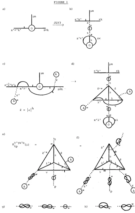
To help obtain a simple form for the RF we digress to the diagrammatic

techniques of Stedman (1975), (1976) - where the details of the following can

be found . The left hand side of (1-13) is depicted by Fig. lea). The stub

on the line labelled K'k' is a 2 jm symbol and z,z', though not group labels,

are left on the lines. The circle labelled 0 is an invariant subdiagram with three external legs and therefore application of the JLVn theorems for

n=3 will reproduce the result of (1-12), Fig. l(b). The top and bottom

parts of this diagram are respectively, a coupling coefficient and a reduced

matrix element, summed over multiplicity indices s,t (dotted lines). The

central part is a permutation matrix or 3 j symbol, m«13), K'~K)st' inserted to produce an 'untwisted' version of the Wigner-Eckart theorem. The diagram

definitions of the two coupling coefficients in (1-14) allow the latter to be

represented by Fig. l(c) with the circles labelled A, depicting those factors

in (1-14). All summations in (1-14) are implied by the diagram. Since

there is a stub on each internal line of Fig. l(c) the whole diagram is an

invariant and the JLV3 theorem may be applied twice, first to the external

legs labelled K'~K, and then to the legs A'~A to produce Fig. led).

Compari-son with Fig. l(b) and (1-15) yields the diagram definition of the RF,

l(e), where we have untwisted the line labelled by irrep

v.

This figure involves a summation over four 3jm vertices and is thus expressible as a 6j

symbol. To obtain the latter in its standard form we introduce further 3j

symbols, the result of the Derome-Sharp lemma, the reality of the 2 jm symbols

and the 2j symbol, ~ , (double stubs). The result is Fig. l(f) with the

(J

corresponding algebraic expression:

KY' ya 'a ( )

tp ~ (AX' _z'r'K' A' Y

J

*

{

~*A'A*}

_{\! K K' t" ,}

s sp

I

.~

KK'

I

~ ~

K \!

x m«132)~*K*K')tt' m«12}\!A'K'*) m«132)v*KA*)

r's' rs

x m(12) ~A' *A) , pp

This result is valid for an arbitrary compact group G. However for our

(1-16)

problems a simplification follows immediately. All the crystallographic

FIGURE 1

b)

K'k'

_I

rm

Kk

a)

JLV3 s·

)

•

.-t

z'K'k' zKk

<D

c)

d)

I~m

K'k' Kk

\.1m

0

cD

•

;r _~

A

•

:t

z'K'k'

*.

ZKk

... ·0

,

,

• r

0~

.

.

#

.

Gj~

*'

K

IKI~

(l)

•

,!,<,.p

x':>'"

@A

e)

_..

.

.

f)

.

:t

(9

KY'YCt'Ct( ) _*'

.

tp )l ₌

.. - *

. .

_•

•

II'¥<

.

'. *

<D

•

~

~

IJ~

.

,

.

.

0*

p

.-r

I ·.r

G~

.

.

'p

_G

g)

··esa~·

..

~;:

··e~·

h)

.. Q ...

[image:16.595.56.531.70.821.2]

11.

the 3j symbols to have a simple form: for an interchange, i, of the columns

of the 3jm symbol (AIA2A3)r~1~2~3 '

± 1. Thus the diagrams . leg) are equivalent. For a

cyclic interchange,

8 rs

and we can neglect the diagrams Fig. l(h) altogether. (Thus the exact

position of a multiplicity line at a 3jm vertex is irrelevant). Even for

groups which are not simple phase i t may be that for the irreps of interest

one can still make the above choices for the 3j symbols. This is the case

for the groups S02' S03' S05 which have been found to be invariance groups

of the vibronic Hamiltonian in special JT systems.

Now, (1-16) becomes

KY'ya 'a ( )

tp J1

I

yv rr,

(AX' A 'YV) _{Z t r ' K '}

*

AXAYV {J1*A' _{zrK V K K}

A.*}

_{t '}

I

KK'

I

~

. r rp

(1-17)

Thus the most general RF can always be written as the sum of two parts: the

first, the A's, contains all the physical information about the

electron-phonon interaction necessary to find eigensolutions of (1-2); the second,

depends upon the irreps of the group G of (1-2) alone. In particular a

knowledge of the 6j, 3j and 2j symbols of G yields all the information about

RFs which can follow from a symmetry analysis, independently of both the

nature and the strength of the interaction V.

As i t is not our intention to attempt a solution of the vibronic problem,

for the remainder of the chapter we treat the A's as free parameters to be

determined for a particular model. But they are not all independent:

orthonormalityof the kets (1-6) a normalization

8

zz'

=

L

XA yvr

by the unitarity of the coupling coefficient. If we set ~

r

l i n (1-17),

the 6j reduces to 11..1<1 (XK*vr').o, the 3j becomes <p, and (1-18) is

rr , 1\

KY'yaa(r )

t=p=o 1 8 zz' (1-19)

1 for any triple (KAv». This result simplifies some of the

3. JAHN-TELLER SYSTEMS OCTAHEDRAL SYMMETRY

In our later chapers strongly coupled JT systems will not be of interest

so we confine our attention to a single degenerate electronic level and its

derived ground vibronic level. Asmost of the studies of the dynamic JTE have

been of systems such as this in cubic symmetry we take the group G to be the

octahedral (double) group O. We investigate the

RFs

which follow for the

2-, 3-, and 4-fold degeneracies that occur, the last of these being sufficiently

complex to highlight the need for a formula as simple as (1-17). We reproduce

the 3j and 6j symbols evaluated by Butler for this group in Appendix IA. We

also.list there the notation used below and throughout our work to designate

irreps and various JT systems. Since for any single electronic and vibronic

mu1tiplets x

=

x', z

z'

and KI = K

=

A'

=

A (certainly for the magnitudes of V we are interested in), we can dispense with most of the labels in (1-17),

rewriting i t as;

I

vrrl

I

y (1-20)

x (>..Avrl) (AA~p)

(the only complex for any point group are those corresponding to Kramer's

doublets but (1-2) is necessarily invariant under time reversal and so has no

matrix elements within these levels, (Abragam and Bleaney (1970».

define a positive parameter,

I

y

We also

13.

(1-18) is then

I

1. (1-22)

vr

We now list the RFs for G 0, A

, r

4,

r

5,

r8

and review previous work connected with them.

3.1 Doublet States -

r3

A

=

f

3

,

~, v

=

r

l

, r2, r3.

There are no multiplicities. We find

1

(We can always remove the

A

label from b

A

without confusion).

v

These equations

give,

(I-23)

With the relabelling q

=

K(r

3), p

=

K(r

2), (1-24) is the most general relation for the RFs of the vibronic doublet, first derived by Abragam and Bleaney and

later by Leurg and Kleiner (1974). Ham's (1968) initial treatment of the

orbital doublet linearly coupled to a single

r3

phonon (pair) of a cluster of nearest neighbours of the ion,

r

3 x £ , showed that b

7

=

0 in the weak and strong coupling limits, a result subsequently generalized by Leung and Kleiner.

They and Halperin and Englman (1973), and Gauthier and Walker (1973) have also

shown that weak linear coupling to lattice phonons of different frequencies

makes b

7 > O. Thus one expects to find for measurements on the vibronic ground state, q < ~ (l+p).

3.2 Triplet States -

r5

A

=

f

5,

r

4 · ~,

v

= f l ' f 3,

r

4' f 5 · Again there are no mUltiplicities. The RF's listed below have the same form for A = _{f5 and f4 so we refer to f5}

throughout only. ( 1-20) gives,

K(r ) b + b

4 - ~ b - ~ bS

3 0 2

K( f

4) b 0

-

~ b4 + ~ b2

-

~ b

s

1 (1-24)

(1-24) is identical to Equn. (37) of Leung and Kleiner. Bersuker and Polinger

(1973) have obtained an equivalent result

in this chapter.

For the linear coupling of the

Ham (1965) obtained the results,

1 ,

the same approach as presented

to a f

3-phonon pair, fS x £,

(1-25)

Leung and Kleiner have since shown that for arbitrary coupling to (many) f3

phonons, that b

2 ~ bS 0, generalizing Ham's result. They also show for weak linear coupling to a fS phonon triplet, fS x T

2, that b2 becomes non-zero only when its perturbative expansion in V is taken to tenth order. Ham

calcul-ated RFs to second order based on the cluster model, for this system, and

Bates et al. (1974) extended his results to full lattice coupling.

These authors and Judd (1974) have obtained analytic expressions in the

strong coupling limit while the intermediate region has been treated numerically,

Caner and Englman (1966), Sakamoto and Muramatsu (1978).

The fS x (£ + T

2' system, coupling to both phonon symmetries, is

more complicated. Originally Bersuker and Polinger obtained RFs on the

cluster model for weak T2 - and arbitrary £-type linear coupling. This work

has since been generalized by Bates et al. One special system exists however,

the equal linear coupling of f3 and fS phonons of equal frequency to the

elect-ronic triplet, fS x (£ ~ T

2). The five-fold degeneracy of the vibrational mode results in (1-2) having symmetry higher than cubic, namely S03 (O'Brien

(1971), Romestain and Merle d'Aubigne (1971». Indeed, as shown most clearly

by Judd (1974), the invariance of the vibrational Hamiltonian under the

oper-ations of the group Us allows the eigenstates Iyvn> to be uniquely labelled by

the irreps of the groups in the chain,

Thus the irreps A, ~, V are those of S03 and are labelled by the J values. For the triplet, A

~

I, and

~,

V = 0, 1, 2. Using $A

=

(_1)2A, (A

lA2A3 0)

15.

K(O) b

+

b

l

+

b

=

1

0 2

K(l) b

+

l:ib - l:ib

0 1 2

K( 2) b - l:ib_l

+

_{10 b 2} 1

0

or

SK(2) - 3K (1)

=

2 - 6b

1

(1-26)

We could have obtained this directly from (1-24) since the 0 irreps are

com-parent labels for the S03 irreps so,

K(l)

=

K(f

4), K(2) (1-27)

(1-26) reduces to O'Brien's result only when b

l

=

O. But she restricted the vibrational quintets to a common frequency. The labelling of the

Us

irreps then insured that J=l of S03 never occurred in the group - subgroup reduction

(Judd) . As no-one has presented the argument clearly we show in Appendix II

that this restriction is removed for quintets of different frequency.

3.3 Quartet States - f8

A

= f8' respectively,

The symmetric and anti symmetric parts of the product

A

x

A

are

f ) 8 s

=

r

₂

+

2f4

+

fS

Thus a mUltiplicity of two exists whenever ~,

v

equal f4 or fS and complex

parameters in addition to (1-21) must be defined,

L

y

(

X3YV]*

A z03

2,5 only (1-28)

They do not appear in the normalization (1-22). Consider now the consequences

of a multiplicity for the matrix element of an operator.

symbolically as,

r

R

r

We write this element

(1-29)

where the bracket denotes a 3jm symbol and ~ is a reduced matrix element. There is a freedom in the way one performs the factorization in (1-29). One

) == U r ' r ' r

(1-30)

R 1 U R

s s's s

where U is a unitary matrix. Then r ~ r ' in (1-29), the matrix element is

unaltered, but the 6j symbols which are formed from the 3jms will be different

for the two sets of labels {r}, {r I} . Now the 6j tables of Appendix IA

corres-pond to one choice for the fS 3jms. However, Butler first produced a

differ-ent set of 6js (unpublished) with which we in turn first calculated the general

form of the RFs for the quartet. This set is reproduced in Appendix IB (the

differences between the two sets only occurs for the triple (332r)). We shall

give our results for both sets of 6js, because, in the first place, we wish to

compare them with the only other major attempt at the fS RFs, that of Ham,

Leung and Kleiner (1976) (HLK) , and in the second place, besides making clear

the arbitrariness of the mUltiplicity choice we want to show that one set of

6j s is preferable for calculations.

For our first set of RFs we use the 6js of Appendix lB. Taking account

of (1-22) and defining B

v

bV + b~ from (1-2S), we can tabulate the results as:

1

K tp (11)

1 -2 -2/5 -S/5 4/5 -2

f3 1 -2 -1 -1/5 -4/5 2/5 -2 -1

r

00

4

1 -2/5

-liS

-13/15 -8/5 -2/5 -6/5 -7/5

U

r

4 1 -S/5 -4/5 -8/5 -4/15 -4/5 -8/5

10f4 4/5 2/5 -2/5 2/5 -4/15 2/15 2/3

01f4 4/5 2/5 -2/5 2/5 -4/15 2/15 -2/3

oarS

1 -2 -6/5 -4/5 -4/15 -4/3 -2/3

1/5 1 -2 -1 -7/5

-8/

5 2/15 -2/3 -1/3

The two remaining RFs not given in (1-31) but produced by our formula are,

K

IO (f 5)

(01)

17.

SEE ERRATA

However, we show in Appendix IlIA that the S03=> 0 3jms require K (r

S) ~ 0 .

tp tp

Thus the eight RFs for the rS multiplet are completely described by eight

real parameters (two of unknown sign) and although one can invert (I-31) to

obtain all parameters there are no

we faced previously.

relations between the RFs such as

HLK restricted the coupling of the ion to the lattice to be linear (of

arbitrary strength) via (many) r3 and rS phonons, rS x (£+T

2), and expressed

their RFs in terms of five parameters. Their (hidden) multipl choice

corresponds to the conventions of Abragam and Bleaney (1970 - section lS.3)

and Koster et al.'s (196.3) coupling coefficients. For future reference we

show in Appendix IIIB that the following one-to-one correspondence between

HLKs labelling of RFs and ours holds as a result:

HLK (1-31)

K .. (r 4)

1.J Ktp (r 4)

where

i,j 2 0

1 t,p 1

K(r~)

K (r 5)

00

K(r~)

Kll(r

S)

K(r

2), K(r3) are the same in both. (Hereafter we use our labelling only). We can also relate two of our parameters to theirs directly (by comparing

(1-6,-9) to their Equns. (1,5) and using Koster et al's tables),

(1-32)

(The numerical coefficients of b

4 and b7 obtained from their RF expressions agree with those of (1-31) with one exception - see below). However, three

relations must exist for the b , B

vr

v

2,5 to obtain their remaining

para-meters. One follows immediately from their results and implies a correction

to one of their formulae without much work on our part: if K

IO(r4) is to depend on the same parameters as the other RFs, as their results suggest, then

we can set BS

=

0 in (1-31) in which case we find K

10(r4) KOI (r4), contrary to HLK. However, as they have this equality to within a factor of 25/9, and

2

their coefficients of pi, b are out by a factor of 3/5 we believe they should

1 2 1

5 (l-p') - 15 (l-q') - 5 a 2

+

!

5 b2 (1-33)

We now turn to the presentation of our second set of RFs using the

6js. of Appendix IA. We first explain why these 6js are a better set to

work with and what effects the transformation between the two sets have.

Amongst the 6js responsible for the formulae (1-31) are those of the

type ,

{1133} 233 . trsp

Here the 'off-diagonal' mUltiplicity pairs (rs) = (10), (01) complicate the

summations in (1-30). If one could remove such pairs then unnecessary work

would be eliminated and, as one simplification, B2 would not appear in K

t t(l1). Butler noticed that for some pairs (t,P) such a transformation of the 6js of

Appendix IB was indeed possible.

tities, i t takes the form,

Denoting the transformed set by primed

quan-{

u

U

r ' r s's (1-34)

where the left hand side is chosen to be diagonal in (r's'). (~ is derived in

Appendix IIle). Notice that this transformation only affects the original set

of 6js whenever the triple (233) is involved. It follows from (I-30) that

any quantity depending upon this triple will also be altered in the multiplicity

separation. Thus in our new set of RFs there will appear new parameters b' 2r, B; , which can be related to the originals by,

[A X3Y2

]

zr'3 U r ' r A

x3y2

zr3 (I-35)

and new RFs, K~'pl

(f

4), obtained from their originals by the transformation (I-34) . All other quantities are unaltered. With these changes our second

19,

1 b

7 b4 b20 b21 bSO bSl

K (fi ) tp

r

2 1 -2 -2 -2

r3 1 -2 -1 -1 2 -1

, r

00 4 1 -4/3

-4/

3 -4/3 -4/3

'II r 4 1 -2 -1 -4/3 -1/3 -2/3 -S/3 (I-36)

r

00 S 1 -2 -4/3 -2/3 -4/3 -2/3

11 r S 1 -2 -1 -4/3 -S/3 -2/3 -1/3

and Kio(r₄) 2/3 (B'

2

+

BS) 01

The simplicity of the expressions (I-36) in comparison to those of (I-31) is

obvious. Six of the RFs are now expressed in terms of six positive parameters

and are independent of the remaining two factors. And although (I-36) and

(I-31) are physically equivalent and the experimental problem of determining

all RFs is not altered by our transformation, the form of (I-36) suggests that

any attempt to find relations between them on a specific model will be made

much easier by using the new set of 6js rather than the old set.

The last problem in this section which may be easily handled by our

formalism is the equal linearly coupled system rS x

(E=T

2) (Pooler and O'Brien (1977), Judd ( 1976) ) • The vibronic Hamiltonian is now invariant under the

operations of the group SOS and the vibrational part under Us ~ 50 S' notation of Appendix IV where the necessary j symbols are listed,

A

fi, V

=

0,1,2. We find the RFs to be

K(l) 1 S/S b

l - 4/S b2

K(2) 1 - 4/S b

l - 6/S b2

or K(2) lo:! {l+K(l)} - 4/S b

2

In the

lo:!,

(I-37)

a result of the same form as (1-23).

determine that,

The compatability relations for SO ~o

5

K(l)

K (2) =

K (r S) 00

SH ERRATA]

and K(2 ) K (f

4)

00

The last two equalities must hold for either multiplicity separation in 0) • (1-37) reduces to the results of HLK and Pooler and O'Brien only when b

2

=

0, which is a special case, by the argument in Appendix II.

4. EXTENDED MULTIPLETS

Section (1.3) dealt with the case of single electronic and vibronic

multiplets, applicable to the study of the DJTE. For a better description of

the JT systems excited vibronic levels must be included, certainly in the

strong coupling limit (assuming that the interaction V is not only linear in

the displacements of the lattice). In theory (1-17) allows

arr

electronic and their derived vibronic states to be included in setting up an effective

Hamiltonian (whose eigenstates will generally involve mixtures of the IZKk»

to describe the effect of (1-10) on the system. (Though in the systems of

usual interest (orbital electronic states) the effects of excited electronic

levels can be neglected in the formation of vibronic as the latter are

typically separated by the order of phonon energies, much smaller than the

electronic separations).

these problems as well.

We can extract all the symmetry information in

As an example, consider an electronic doublet x=x',

>,,=>"'=f •

3 The

possible vibronic irreps are

K,K' = (f

l

,f

2

,f

3) and there will be five RFs with fixed

z,z'

for ~

=

f f

3. Ham (1972) uses the RFs corresponding to the first 2,

excited singlet

(K'=f

l

/f

2) connected to the ground doublet

(K=f

3), r in his

notation, to describe the transition to the static JTE. However, the only

RFs that can be related have the

K,K'

labels in common, for all·systems.

Thus for

K=K'=f

we find, 3

K2 '2(f 3)

x4y7 Az4

- a generalization of (1-23) to include all vibronic levels of f3 symmetry

21.

of the previous section will generalize like this. Also there may exist

additional relations for vibronic levels of other than ground state symmetry.

The triplet

A

=

A'

and

where y'

KY'Y(f ) 5

(z

)

.

y'

y

o

y

A knowledge of the vibronic levels structure and the non-zero parameters for

specific JT interactions would allow the above relations to be exploited in

determining the effective Hamiltonian for any system, in the manner of Setser

and Estle for the orbital doublet. We shall not pursue these problems, as

our answer to an effective Hamiltonian description for the external

perturb-ation will turn out to be quite different.

s.

SUMMARY

The most general group-theoretic construction of the eigenstates of

an arbitrary ion-lattice Hamiltonian, and a general definition for the RFs

corresponding to an external perturbation, has led to an expression for these

RFs, (I-17). The symmetry information inherent in their definition can now

be simply extracted, given the 6j symbols of the invariance group. Unlike

previous, and less general, formulations, our method emphasizes the basis

independence of the RFs. Also, i t easily handles systems of any complexity:

from a symmetry viewpoint, we have given the first complete treatment of the

RFs for the fa states. Vibronic RFs will not be of specific interest to us

in succeeding chapters. However, the relations between the ground state RFs

will be, in particular, those for the r

3, fS, ra,systems listed in Section (I.3). (For the f8 states there are a number of possibilities, depending upon which

parameters b we choose to display) • We shall refer to any special relation,

\!r

appropriate to less than arbitrary coupling for example, or when one or more

CHAPTER II

REDUCTION FACTORS VIA GREEN FUNCTIONS

We review the formalism necessary for a quantum field-theoretic

description of the interacting ion-phonon system which yields one-particle

properties of the system, for example level shifts (eigenvalues) and widths

(lifetimes) . This description obviates prior knowledge of the eigenstates

of the electron-phonon system. We then follow Gauthier and Walker (1976)

and find the effect of the external perturbation on the eigenvalues of the

system. However our analysis is quite general. We represent all the

alge-braic parts of the formalism by Feynman graphs and we show how the symmetry

information in these graphs may be revealed. This allows the most general

(electronic) reduction factor to be defined as the sum of a series of diagrams.

We compare the Green function method with that of the previous chapter.

1. A PERTURBATIVE SOLUTION FOR THE ION-PHONON SYSTEM

1.1 The Green Function Formalism

As Thermal Green function and diagram techniques are discussed fully

in the literature (Abrikosov e t a l . (1963), Fetter and Walecka (1971», we

only outline here those ideas necessary for an understanding of the formalism,

as i t applies to our problem.

Our electron-phonon system consists of an isolated impurity ion coupled

to the continuum of lattice vibrations of a host paramagnetic crystal. In

second quantized form the zero order Hamiltonian for the non-interacting

system can be described by,

H o

=

I

i

+ H P

t

E.

1 a. 1 a. 1

+

I

k

(11-1)

The fermion operators

a~(a.)

create (annihilate) the ionic level Ii> of

1 1

23.

SEE ERRAT~_

of energy E with wavevector k in the Brillani zone and belonging to branch k

mode s, k ks) (k :: (-~,s». The coupling V of (1-2) is to be treated as

a perturbation on the system of (11-1). It can take various forms but we

restrict i t to linear coupling in the meantime,

L

ijk

V V _ijk at a '"

i j 'f_k ( II-2)

~k

= b

k + bt is the phonon displacement operation and Vijk the coupling para-meter.

where T

Define a full one-particle electronic Green function

G . .

(T) by,

l.J

G . .

(T)

-

<T {a. (T) a~}> T

it/t

l.J T .1. _J

is the 'time' ordering operator, a. (T) is a Heisenberg operator

T .1.

OCT) e HT 0 e -HT

and < ..• > denotes a thermal average with respect to H,

<A> =: TrpA

P

= e -8H/ Tre

-BH

(II-3)

(II-4)

The significance of (11-3) lies in the fact that i t describes the propagation

of excitations of the electronic subsystem in a 'time' interval T allowing for

all possible interactions with the phonon subsystem. Thus G .. (T) is

proport-.1..1.

ional to the probability amplitude that the excitation at 10> will not decay

.1.

in a time T and hence the state Ii> acquires a finite lifetime as a result of

interactions.

A consideration of the time development of the system in the interaction

representation for the operators (H 7 H in (11-4» yields, o

Here

G . . (T)

l.J

5(8)

<T {S(8) a. (T) at }> /<5(8»

T .1. J 0 0 (II-5)

is the S-matrix and < ..• > denotes averaging with respect to H. (11-5) is

o 0

a perturbative expansion to infinite order in V. At this stage in the usual

theory of a many fermion system one proceeds by applying Wick's theorem to

of the subsystems,

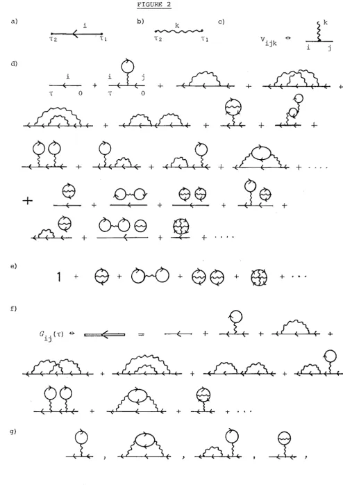
( II-6)

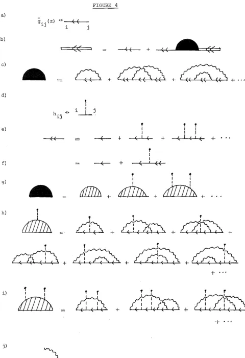
If these propagators are represented by the diagrams in Fig. 2(a),(b)

respect-ively, and the interaction by the vertex 2(c), then i t can be shown the

numer-ator and denominnumer-ator of (11-5) have the respective diagrammatic expansions

2(d) ,(e), where, in order to reproduce all the terms in (11-5), all possible

ways of connecting the propagators (11-6) are employed. For example, 2(d) ,(e)

contain all diagrams to fourth order in

v.

The advantage of the physical

interpretation of each diagram in terms of the creation and annihilation of

virtual phonons changing the character of the bare electronic levels, is obvious.

Rather than evaluating the contribution of each (Feynman) diagram to

G ..

(T) (by integrating over T. variables, summing vertices over state variables

1J 1

etc.) a simplification is made at this point. 2(d) consists of two classes

of diagrams; connected (the first 12) and disconnected (the remainder). The

T.-integrations in the latter factorize. Cancellation of the diagrams common 1

to 2(d) and (e) then occurs - this can be seen intuitively - and

G . .

(T) can be

1J

rewritten as 2(f), the sum of all topologically distinct, connected diagrams

-the linked cluster -theorem.

Now we return to the one-particle system under consideration. The

vacuum state 10> and states occupied by more than one fermion e.g. at at 10>

1 J

(i~j) are not physical states of the ion. To eliminate their contribution when

evaluating quantities like-;:'A> in (11-5) Abrikosov (1965) added an extra o

energy 6 to each ionic level,

for the one-fermion states (1)

operator (Keiter (1971»,

p

~ (E.+6) 8. in (11-1), and removed its effect

1 1

at the end of the calculation via the projection

lim 8-<x>

e

S8

p <A> ~ <A>

o all states 0 1

The effect of P on the numerator of (11-5) is to eliminate all those diagrams

in 2(d) containing one or more fermion loops (e.g. 2(g» and the linked cluster

a)

d)

e)

f)

g)

h)

FIGURE 2

b)

c)

25.

~k

V"k

**

- L

1J i _j

( i

+

&

4-

(0 (

+

(~(

+

(~.

+<

(~/~.

+

X

+

2

+

n

+

k

4-

~

+

,6\,

+ ....

+

~

+

0;0

+

0(

$

+

~

+

G, ,CT)

**

1J

+

( I =

ill

+ ---'--

+ ....

(

(C'l£':'., (

+

,~,

+

J::l/'0(

+

d

~

+

,tn,

+

Y

+ . . .

-2

~,~

-i,

i

« . ""

j

"

[image:31.597.53.547.58.755.2]

~E ERRATA

act essentially as a normalization factor and have no effect on the quantities

we wish to calculate (McKenzie (1978», so we ignore them. The resulting

diagram expansion of G, ,(c) for the electron-phonon system reduces to 2(h).

1J

The Fourier transformer of (11-3) is now taken:

f

s

z\l'

G,,(zV):: dTe G,,(,), z

1J 0 1J

v

Corresponding definitions for (II-6) give,

1

d (x )

n V

1 X -E:

\I k

1

x

V

in

2V-S

(II-7)

(II-8)

These functions are defined only at discrete 'energies' z , x , (the subscript

V \I

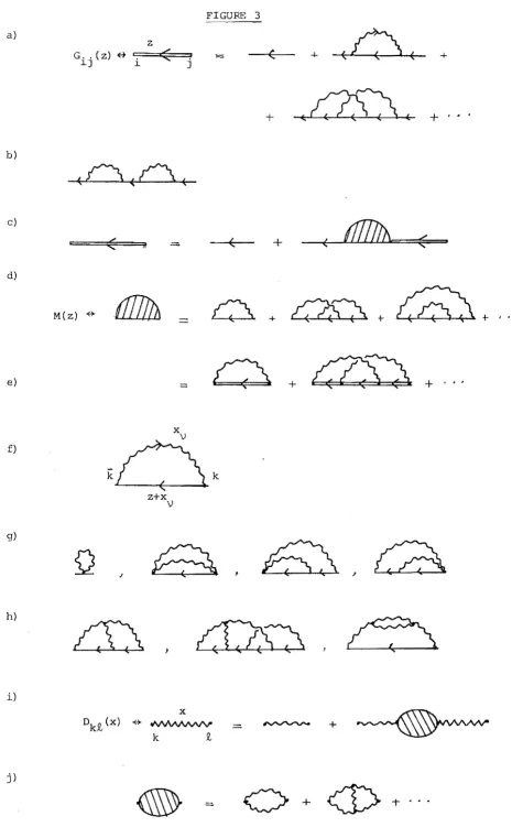
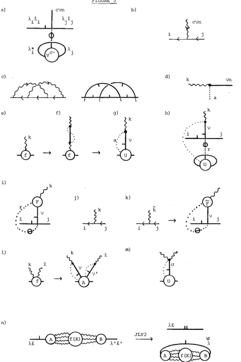
\I will be dropped in the following). Now G, .(z) is also represented by the

1J

series 2(h) but with, replaced by an 'energy' z which must flow through each

diagram - Fig. 3(a}. The advantage of working with the Fourier transform is

that diagrams like Fig. 3(b} factorize in their contribution to G" (z). This

1J

results in the iterative Dyson equation.

equation is, in operator form,

G(z) = g(z}

+

g(z} M(z) G(z)

Defining G. , (z)

1J <iIG(z}

Ip,

this

(II-9)

where g (z) is diagonal in the basis

{I

i>}. (II-9) has the diagrammatic

rep-resentation of 3(c). M(z) is the self-energy operator consisting of the sum

of all irreducible diagrams, 3(d), - those diagrams in G(z} which cannot be

factorized - and can be written most compactly as 3(e). If the inverses of

the operators g(z), {l-g(z) M(z)} are defined, (II-9) can be rearranged to,

G(z) {(g(z»-l - M(z)}-l

{z - H

e - M(z)} -1

(II-IO)

Although the complex functions G(z), M(z) are defined only at discrete points

along the imaginary axis I after evaluation (by rules to be given shortly) they

can be analytically continued to the whole complex z-plane, in particular to

the real axis I z ~ E

±

io (Fetter and Walecka) .

~(E), r(E) may now be defined via,

-M(E ± io} ~(E)

+

i f(E)

Two Hermitian operators

a)

b)

c)

d)

e)

f)

g)

h)

i)

j)

FIGURE 3

z

G .. (z) tf+ i . ( , =

~J ~ j

==(~~!'

-M(z) #

k

Q

j

z+x

V

x

DkQ, (x) # tN\AA.IvvVV k Q,

k (

27.

+

+

+ ...

+

(

,

.

,

[image:33.597.60.526.64.826.2]

Restricting G(z) to diagonal elements for simplicity G, , (z) 11 near the poles (11-10) gives,

G, (E±io)

1 {E - 8, 1

!:", (E) ± i f, (E) }-l

1 1

G, (z), then 1

(II-12)

The interpretation of (11-12) is as follows: when

V

=

0, the state

Ii>

has an energy 8, (the pole of g, (z»; for V

f

0, the energy is given by the solution

1 1

of,

E - 8, - !:", (E)

1 1

o

(II-l3)

and defines a dressed excitation shifted in energy from the bare state. In

the Lorentzian approximation in which the arguments of !:"" f, are made

indep-1 1

endent of E (in its simplest form E ~ 8, in the argument, but see Stedman 1

(1971), Hernandez and Walker (1972», this 'quasiparticle' decays with an

inverse lifetime ~ f,(e,) (Abrikosov et al). We refer to this as the width

1 1

of the excitation since the spectral function describing the excitation is a

Lorentzian of half-width f, (e,), peaked at 8,

+

!:", (8,), in this approximation

1 1 1 1 1

(Stedman 1971).

Thus

!:,,(E), feE)

are interpreted as shift and width operators respectively

for the totality of ionic levels under consideration.

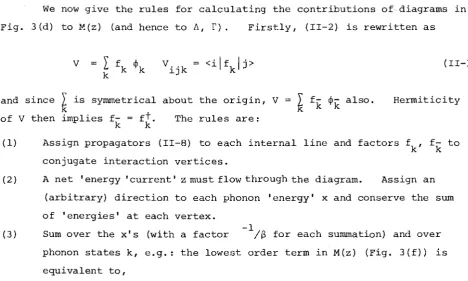
We now give the rules for calculating the contributions of diagrams in

Fig. 3(d) to M(z) (and hence to !:", f). Firstly, (II-2) is rewritten as

V

I

k

V

k (II-14)

and since

k

is symmetrical about the origin, V implies f- = ft. The rules are:

Hermiticity

of V then

k k

(1) Assign propagators (II-8) to each internal line and factors f

k, fk to conjugate interaction vertices.

(2 )

(3)

A net 'energy 'current' z must flow through the diagram. Assign an

(arbitrary) direction to each phonon 'energy' x and conserve the sum

of 'energies' at each vertex.

Sum over the x's (with a factor -1

/p

for each summation) and over phonon states k, e.g.: the lowest order term in M(z) (Fig. 3(f» is

[image:34.595.65.534.506.787.2]

1

B

I

x\lk

29.

(4) Convert the sum on x to a contour integral over the complex x-plane

\I

and evaluate by the method of residues (Fetter and Walecka, Schreiffer

(1964» .

Since the residue of the pole of g (z+x) vanishes as

e

-+::0, the sum reduces to,

1

I

B

x

\I

~

{e6Ek - l}-l is the Bose-Einstein population factor.

Although individual diagrams are most easily calculated by the above

rules, a little thought shows that each diagram in Fig. 3(d) is reproduced by

a term in the expansion of

co

M(z)

=

I

(II-IS)

n~o

Here Ip> is an eigenstate of H and the thermal average is over all excited p

states of the lattice:

Hlp>

p E p Ip>

-6Ep/

-6Ep

e Tr e

Only irreducible diagrams are to be included in the summations.

Finally we note that interactions other than (11-2), hereafter denoted

as

VI'

are easily dealt with by the appropriate diagrams.

quadratic interaction,

For example the

(II-l6)

contributes diagrams like Fig. 3(g) to M(z). (In future we shall not draw

the mirror image of an asymmetric diagram as in 3(g) but i t is understood to

be included). And if we relax the approximation of

a

.harmonic crystal the

(lowest order) anharmonic phonon interaction,

1

31.

I

kR.m

gives diagrams like 3(h). Strictly though,the last diagram in 3(h) will be

included in a full phonon propagator Dk~(xV)' also obeying a Dyson equation,

3 (i) ,

D(x) d(x)

+

d(x) P(x) D(x).

The phonon self-energy P(x), would then correspond to the series 3(j), where

electronic loops are now eliminated by the Abrikosov procedure. The effect

of the replacement of the unperturbed propagations d(x) in 3(d) by D(x) would

be to change the value of

E

corresponding to H no longer being in the harmonic

p p

approximation. We ignore these corrections.

1.2 Comparison With the Standard Procedure

Much of the literature concerned with perturbative solutions to the

electron-phonon problem uses the method of section (1.1) - explicit construction of the vibronic eigenstates. We compare this method with the Green function

approach. Firstly we note the effect of symmetry restrictions for the latter.

We have in mind that the electronic Hamiltonian, H =

~ e.a~a.

will represent e l l ]. 1

a sequence of multiplets, not degenerate with one another, each of which may

be labelled by the irreps of the symmetry group of H , Ii> = IX.A.~.>. The

e l l ].

interaction

V

will modify the energies of these multiplets according to the

solutions 0 f ,

(E - H - ~(E) Ii»

=

0 e

where Ii» is a vector constructed in the basis {Ii>}.

(II-18)

This is just the

generalization of (II-13) to include the off-diagonal elements. Since

V

and

H are invariant with respect to the symmetry group so is (11-15), and there-o

fore ~(E). By Schur's lemma (cf. (II-39»,its matrix elements have the form,

f(E,x.x .. ,A.) 0 \

on n

1 J 1 AiAj kikj

and the shifts in energies will be the same for all the components ~. of a 1

particular multiplet. Thus the electronic degeneracies are retained when the

interaction is switched on.

Suppose we follow the usual procedure and construct exact eigenstates

{Iy,> :: IZKk>} of H =: H +V from the product states {la>18>

=

IXA~>lyvn>} of H .

o ' 0

We can use the results of Brillouin-Wigner perturbation theory (Ziman (1969»

adapted for this problem. For simplicity we consider a single electronic

state, but many vibrational states 18 >, a

=

1,2, •.•

zero-31.

order states la>ls> , of energy Eo ' the eigenstate Iy > of H is given by,

a a a

0 )

[E_IH

pvt

jy

>

_L

la>IS > (II-19)

a a

n=o 0

(p = P

a

+

Ps - PaPS' is the complementary projection operator) with the corres-ponding eigenvalue,

E <y

I

H

jy

>

a a a

( II-20)

This also has the degeneracies of the symmetry group. We now construct the

state Iy> Ely>· It is not an eigenstate of H but we assume i t to be a a

approximately so with eigenvalue E E. This is allowable in the sense that a a

one can never specify the eigenstates

h

> precisely. Not only do they evolve a

in time as a result of interactions ((II-19) is the time independent solution},

but the vibrational states Is > can never be specified either - in reality they a

depend upon the temperature of the system. Measured quantities of the system

are in fact (grand canonical) ensemble averages over the

{IS

>}. Performing a

this for (II-20), we see that the change in the electronic energy, E (E -Eo ),

a a a

is just the energy shift ~ (E) obtained from (II-18), (one can replace

-1 _laa

(E-H) .P by (E-H ±io) - Van Kranendonk and Walker (1968». Thus the two

o 0

methods agree within our approximation.

Clearly the construction (II-19) makes i t impossible to know the real

matrix elements of operatOrs. And even assuming that one could calculate

the eigenstates of the time-dependent Schrodinger equation, (a very difficult

task), i t would be quite unnecessary: the one-particle thermal Green function

determines all there is to know about the ensemble averages of observables

corresponding to these operators (Ziman). The time evolution and temperature

dependence of the system is fully incorporated in the Green function. In

addition the coupling of the ion to the phonon continuum can be as complicated

as one pleases. None of this information is so easily available using the

standard procedure (for which reason many of the results have been simplistic) .

Thus whenever a perturbative solution is possible, one can forget about