Coarse grained computer simulation of fibre self assembly

(1)

assembly.

PRYBYTAK, Pavel V.

Available from Sheffield Hallam University Research Archive (SHURA) at:

http://shura.shu.ac.uk/20250/

This document is the author deposited version. You are advised to consult the publisher's version if you wish to cite from it.

Published version

PRYBYTAK, Pavel V. (2012). Coarse-grained computer simulation of fibre self-assembly. Doctoral, Sheffield Hallam University (United Kingdom)..

Copyright and re-use policy

See http://shura.shu.ac.uk/information.html

(2)

I_*JC U ! Ml i y Ctl !U II M l/ l l l l C t l K J ! I I J C I V IV /C O

Adsetts Centre, Citv Campus Sheffield SI 1WD

1 0 2 0 0 6 8 5 6 6

REFERENCE

Sheffield Hallam University Learning m j Information Services

(3)

The quality of this reproduction is dependent upon the quality of the copy submitted. In the unlikely event that the author did not send a com plete manuscript and there are missing pages, these will be noted. Also, if material had to be removed,

a note will indicate the deletion.

uest

ProQuest 10700895

Published by ProQuest LLC(2017). Copyright of the Dissertation is held by the Author.

This work is protected against unauthorized copying under Title 17, United States C ode Microform Edition © ProQuest LLC.

ProQuest LLC.

789 East Eisenhower Parkway P.O. Box 1346

(4)

Coarse-Grained Computer Simulation of

Fibre Self-Assembly

Pavel Prybytak

A thesis submitted in partial fulfilment of the requirements of

Sheffield Hallam University

for the degree of Doctor of Philosophy

(5)

In this Thesis we present the results of a series of molecular computer simula tion studies undertaken to investigate fibre self-assembly. The driving objective for this work has been to develop a generic coarse-grained model for peptide systems and examine its ability to exhibit free self-assembly of fibre structures at moderate computational cost.

Firstly, the development of a model is addressed. The model is based on mixtures of disc-like Gay-Berne and spherical Lennard-Jones particles. The discs represent single-site models of peptide molecules, whereas the spheres represent solvent par ticles. An additional parameter in the disc-sphere potential is introduced to adjust solvent quality. Using this model, depending on variables such as the solvent quality, formation of either chromonic stacks or chiral fibres is observed.

To explore the process of fibre self-assembly in more detail, larger systems are studied. Here, we find that, for a narrow temperature range, defect-free chiral fibres can freely self-assemble from an initially isotropic configuration. This occurs as a result of a complex multistage process, which can be controlled by adjusting the temperature. We study systems with different disc-disc interaction strengths and find that this parameter can be used to control the size and shape of a resultant fibre. We also investigate whether chiral fibres have a limiting radius.

(6)

The Road Not Taken

Two roads diverged in a yellow wood, And sorry I could not travel both And be one traveler, long I stood And looked down one as far as I could

To where it bent in the undergrowth;

Then took the other, as just as fair, And having perhaps the better claim, Because it was grassy and wanted wear

Though as for that the passing there Had worn them really about the same,

And both that morning equally lay In leaves no step had trodden black.

Oh, I kept the first for another day! Yet knowing how way leads on to way, I doubted if I should ever come back.

I shall be telling this with a sigh Somewhere ages and ages hence;

Two roads diverged in a wood, and I -I took the one less traveled by,

And that has made all the difference.

(7)

I would like to thank my supervisors, Prof. Doug Cleaver, Prof. Chris Care and Dr. Tim Spencer for their support and guidance during this project. Thanks also to my former supervisors in Belarus, Prof. S.V. Hileuski and Prof. V.V. Apanaso- vich, who encouraged me making the decision to study in England. I also wish to acknowledge the support of the Unilever and the Materials Research Institute at Sheffield Hallam University for providing a student bursary.

It gives me pleasure to thank all of my colleagues whom I have worked with over the past three and a bit years. So thanks to Alex Webster, Terry Hudson, Mish, Tim, David Michel, Vinay, Stuart, Vic, Mike. I am also very greatful to all my friends, who assisted me and who have made my stay in Sheffield so enjoyable and memorable. Thank you Alex, Mish, Jan, Vitald, Andrei, Lesha and Ira, Jurij, Alibek, Gena, Taras, Sasha, Viktor, Katya, Eugenia, Pavelas, Sol, Vinay, Julia, Ann, Max, Sofia, Richard, Steve, Alena.

(8)

Advanced Studies

The following is a chronological list of related work undertaken and meetings attended during the course of study:

• IOP Winter School, Leeds, January 2009

• MERI Research Methods module, Sheffield Hallam University (2009)

• IOP Biological and Soft Matter Conference, Warwick University, April 2009

• MERI 1st Year Student Seminar Day (Poster Presentation)

• CCP5 Summer School Sheffield, University of Sheffield, July 2009 (Poster

Presentation)

• NASQ Meeting, Warrington, 11 September 2009 (Oral Presentation)

• Course in MPI, HECTOR, Exeter, 14-16 September 2009

• MERI 2nd Year Student Seminar Day (Oral Presentation)

• CCP5 Annual Meeting, Sheffield Hallam University, 13-15 September 2010

(Oral Presentation)

• NSASM International Workshop, September 20-24, 2010, Dresden, Germany (Poster Presentation)

• BLCS Annual Conference, University of Nottingham, April 2011

• Geometry of Interfaces Conference, Primosten, Croatia, 3-7 October 2011

(9)

Chapter 1

Introduction

Due to their unique ability to undergo reversible and discontinuous system-wide phase change in response to different external physicochemical factors, fibre-forming systems have found broad application in various technological and biomedical appli cations. For example, hydrogels have been extensively used in the development of smart drug delivery systems. A hydrogel can be considered as a three-dimensional network of crosslinking fibres. Loaded with drug molecules these structures may release payload in response to changes in the local environmental conditions, such as pH, temperature, presence of small molecules or enzymes, and oxidising/reducing environment, among others. Hydrogels are also of great interest as a class of materi als for use in tissue engineering and regeneration as they offer 3D scaffolds to support the growth of cultured cells. Another key application is in bio-sensing, where small chemical or physical changes in the sensing environment trigger macroscopically ob servable changes in material properties, thereby reporting the former, for example by gelation or nanoparticle assembly [1].

The practical importance of fibres’ applications has attracted considerable at tention to this class of materials. However, even though many experimental and theoretical studies have been performed on such systems, a complete understanding of their supramolecular structure and the way in which they form has yet to be

(13)

achieved. The relative complexity of the molecular units which form fibres via the processes of self-assembly, makes a full theoretical description of these systems a formidable challenge. Further, empirical observation of these macroscopic phenom ena requires high spatial and temporal resolution, inaccessible to many experimental techniques. This means that computer simulation has the potential to be an effec tive tool here, bridging the gap between experiment and theory, and giving novel insights into the molecular basis of fibre formation.

1.1 Aims and Objectives

The work presented in this Thesis addresses the study of fibre self-assembly by means of molecular simulations. The aims of this study were set as follows:

• to research the self-assembly processes involved in fibre formation, in terms of a generic molecular model.

• to develop a generic coarse-grained model able to exhibit free self-assembly of fibre structures at moderate computational cost.

• to implement this model via an appropriate simulation strategy.

• to conduct a detailed study of fibre self-assembly using the developed model and associated analytical methodologies

1.2 Outline of the Thesis

The Thesis is organised in eight Chapters, including this brief introduction.

(14)

CHAPTER 1. INTRODUCTION 3

results presented here, although some effort has been made to give a wider consid eration.

Chapter 3 reviews computer simulation techniques relevant to the study per formed here. A particular emphasis is placed on the Molecular Dynamics (MD) simulation method used in this project. This chapter also describes two important soft particle models: the Gay-Berne and Lennard-Jones model.

In chapter 4, model development and testing is described. An initial molecular model is introduced and preliminary results associated with this model are presented.

Following from these initial results, Chapter 5 presents comprehensive results of simulations of much larger systems. Systems with different parametrisations are studied and the resultant data are analysed. From this, a detailed description of the processes involved in fibre self-assembly is given.

In chapter 6, a modified version of the model is introduced in order to investigate self-assembly of aggregates which incorporate solvent particles within their struc tures. This modified model is then used to study how these composito-structures vary with model parametrisation. Following from these initial studies, Chapter 7 presents results of additional simulations of some of the systems from Chapter 6, conducted in constant NPT ensemble.

(15)

Chapter 2

Studies of fibre self-assembly

The study of molecular self-assembly has become an active and diverse field of research, ranging from biomedicine and biotechnology to material science and nan otechnology. Understanding of the sequence-structure-properties relationships in self-assembling systems is crucial, in view of the rational design of new nano build ing blocks for biotechnological applications or new drugs. Special interest has been shown in self-assembling biodegradable materials based on proteins, polysaccharides and polypeptides [2]. This class of biological materials has considerable potential for a number of applications, including scaffolding for tissue repair in regenerative medicine, drug delivery and biological surface engineering [3]. A significant amount of existing research in the field of molecular self-assembly has been concentrated on peptide self-assembling systems. The relative simplicity of structure, simplicity in design and synthesis, make peptides an attractive model system for the study of fibre self-assembly.

2.1 Experimental studies of fibre self-assembly

Short aromatic peptides have been found to self-assemble into a number of different supramolecular structures such as straight hollow spherical structures, amyloid-like

(16)

CHAPTER 2. STUDIES OF FIBRE SELF-ASSEMBLY 5

fibres and nanotubes. These were first described by Reches and Gazit et. [4, 5]. Although a complete understanding of the self-assembly of these peptides has not yet been achieved, some intuition has been gained. For example, aromatic interac tions (or 7r — 7r interactions) are believed to play a key role in the formation of these

structures, TT — 7r interactions are attractive interactions caused by intermolecular

overlapping of p-orbitals in 7r-conjugated systems. Obviously, the larger the num ber of 7r-electrons, the stronger the interaction is. Thus, surfaces of flat aromatic rings tend to arrange themselves in stacks, contributing a free energy of formation, as well as order and directionality, to the self-assembly process [6]. Besides aro matic interactions, hydrogen bonds and ionic interactions are also present, but their contribution is less understood and explored.

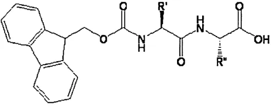
Fmoc-dipeptides belong to a class of aromatic peptides. They comprise a Fmoc (9 -Fluorenylmethoxycarbonyl) protecting group and two chemical residues (the generic molecular structure of Fmoc-dipeptide is presented in Fig.2.1). By varying the chemistry of the residues, different peptides can be synthesised. For instance, if Phenylalanine is used as a residue Fmoc-Phenylalanine -Phenylalanine peptide will be synthesised. It is noteworthy that this peptide is believed to represent the smallest structural unit that can form typical amyloid-like fibres [6].

O

"OH RB

Figure 2.1: Generic molecular structure of Fmoc-dipeptide.

[image:16.612.181.448.496.605.2]

(17)

for a range of these peptides, although in some cases (Fmoc-glycine-phenylalanine and Fmoc-glycine-threonine) no gelation was observed under any of the conditions tested, crystals being formed instead. CryoSEM images of the thus synthesized gels shows significant morphological variation (Fig. 2.2), indicating dependence on the amino acid sequence in the peptide. The diameters of the fibres that were observed by Ulijn et al.[7] for all peptides are summarized in Table 2.1.

Fmoc-peptide pH Fibre diameter [nm

Gly - Gly < 4 33 ± 8

Ala — Gly < 4 30 ± 6

Ala — Ala < 4 68 ± 18

Leu — Gly < 4 22 ± 5

Phe - Gly < 4 25 ± 6

Gly - Phe — —

Phe — Phe < 4 56 ± 13

Table 2.1: Diameters of the Fmoc-dipeptide fibres presented in [7].

Figure 2.2: Morphology of the Fmoc-dipeptide gels observed in [7].

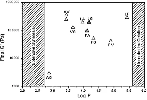
The influence of the hydrophobicity of the Fmoc-dipeptides on their gel proper ties has been studied at Unilever Research. Storage moduli reported after 20hrs are plotted versus logP (hydrophobicity) in Fig. 2.3. These results further indicate that the molecular structure of peptide has a direct effect on the resultant gel properties.

(18)

CHAPTER 2. STUDIES OF FIBRE SELF-ASSEMBLY 7

Fmoc-peptide Ri R2 LogP

Ala — Gly CH3 H 2.865

Ala — Val CHS CH (C H 3)2 3.431

Val - Gly CH3CH {CH3)2 H 3.644

Leu — Ala CH2CH {CH3)2 c h3 3.962

Phe — Ala CH2Ph c h3 4.113

Leu — Gly CH2C H (C H 3)2 H 4.175

Phe — Gly CH2Ph H 4.326

Phe - Val CH2Ph CH (CH 3)2 4.892

Leu — Phe CH2CH{CH3) 2 CH2Ph 5.423

Table 2.2: Fmoc dipeptide sequence studied at Unilever Research along with their hydrophobicity (Log P).

toooooo LF VG F A CO CL FG F V O <T3 ,C _toooo -u_

A G

1000

2.5 3 JO 3.5 45 5.0 5.5

2.0 4.0 e jo

Log P

Figure 2.3: Storage moduli versus hydrophobicity for the dipeptides listed in Table

2.2.

large degree of ir — TT stacking of the fluorenyl group, suggesting that aromatic inter

actions have a significant influence on fibre self-assembly. Based on these features, it was assumed that fibres are formed from twisted antiparallel /^-sheets, interlocked via 7r — 7r stacking of fluorenyl groups.

[image:18.612.189.426.264.426.2]

(19)

4L Single ribbon ^

Tom ribbon \ magnified

Overlapping ribbon* form a moth

*

Cluster of ribbons

*

Figure 2.4: TEM image of Fmoc-Phe-Phe gel [9], showing an overlapping mesh of flat ribbons.

to be in good agreement with the proposed model structure of [9].

As can be seen from examples above, experimental techniques make it possible to study and analyse the structure of formed fibres. However little is known about the early-stages of fibres self-assembly, due to limitations of available resolutions. Nevertheless, some progress in this direction has been established. Different exper imental reports suggest that fibre self-assembly is a multi-stage process involving distinct intermediate structures.

(20)

CHAPTER 2. STUDIES OF FIBRE SELF-ASSEMBLY 9

but that later they detoxify by conversion to a fibre [11, 12].

An interesting example of combining experimental techniques with computer simulation to study fibre formation has been presented by M. Marini and co-workers [13]. They studied the self-assembly of the eight-residue peptide KFE8. Depend ing on the ionic strength of the solution, different rates of self-assembly could be achieved. The pH of the solution was, therefore, adjusted such that speed of self- assembly was considerably reduced, making it possible to study intermediate struc tures. AFM images and electron microscopy performed on quick-frozen aliquots taken from evolving solutions then confirmed the presence of left-handed helical ribbons a few minutes after preparation of the peptide solution. After 2 hours, the concentration of these ribbons decreased considerably and further assembly into bands of parallel filaments was observed. CD spectra collected over time indicated a steady increase in antiparallel /3-sheet structures in the early stages, followed by decrease in the presence of random coils. This suggested that ribbons are interme diates in the formation of fibres. Various /3-sheet configurations were constructed and their stability was tested by all-atom MD simulations. Dimension and pitch of the most stable simulated configuration was found to be in a good agreement with experimental measurements.

(21)

used to estimate dimensionality of growth and the size of the nucleus. According to this analysis, the critical nucleus comprised six to eight partially folded dimers. Af ter nucleation, subsequent linear fibre growth occured through both elongation and thickening. The first fibres were visible by TEM at 10 to 30 min. At later times (1-2 hours) it became possible to observe fibre elongation directly by LM. Additionally, a series of seeding experiments was conducted. In this, fragmented matured fibres were used as initial nuclei. These produced more and shorter fibres with increasing amounts of seed.

ms______________ min________________ hr_________________________day

Figure 2.5: Schematic of possible pathways for fibre formation. (A) The two peptides may interact to form various oligomers that are competent for fibrelogenesis, or (B) the individual peptides may be competent for assembly. (C) Onward assembly may be immediately energetically favorable, or (D) further assembly may only be favorable once a critical nucleus has formed. (E) fibres may thicken via the bundling of fibres, or (F) the addition of material in both radial and longitudinal directions

yields mature fibres as shown in the electron micrograph (scale bar: 5 fim). The

(22)

CHAPTER 2. STUDIES OF FIBRE SELF-ASSEMBLY 11

2.2 Computer simulations of fibre self-assembly

Self-assembled fibre nanostructures hold great promise for many applications. How ever, even though many experimental and theoretical studies have been performed on such systems, a complete understanding of their supramolecular structure and the way in which they form has yet to be achieved. The relative complexity of the molecular units which form fibres via the processes of self-assembly, makes a full theoretical description of these systems a formidable challenge. Further, empirical observation of these macroscopic phenomena requires high spatial and temporal res olution, inaccessible to many experimental techniques. This means that computer simulation has the potential to be an effective tool here, bridging the gap between experiment and theory, and giving novel insights into the molecular basis of fibre formation.

However, the inherent potential of this approach is limited by the time and length scales that can be accessed. Depending on the complexity of the building blocks and size of a system, the time scale of a processes such as fibre self-assembly is on the order of seconds, to minutes. In comparison, most MD simulations are limited to times on the order of nanoseconds. Statistical sampling (such as in MC simulation) would also require significant amount of computational resources due to the large configuration space needed to be explored in order to equlibrate and sample self assembled nanostructure. Thus, a rigorous numerical study of this problem at the atomistic level is beyond the capability of modern computers. For this reason, in most of the presented full-atomistic simulations studies of molecular self-assembly, number of molecules (building blocks) used is limited to dozens and, in some cases, pre-assembled structures are used and tested for stability.

(23)

in MD simulations to study their self-assembly into a chromonic stack. Despite the number of molecules being small, it took 200 ns to observe system evolution from the initial dispersed state through formation of dimers and tetramers to development of single stack of eight molecules. Subsequently, using preformed 9 stacks of 16 molecules each, larger simulations were used to investigate chromonic columns with a loose hexagonal packing, corresponding to a nematic phase of SSY.

Often, an atomistic simulation is used just to verify the stability of a constructed (or preformed) nanostructures. Typically this approach involves constructing a wide variety of molecular packing geometries that are consistent with the dimensions found experimentally. Each of these is then evaluated by MD simulations to identify the most stable one [16, 17]. This approach enables determination of structural features as well as significant interactions that stabilize the nanofibre [18].

The limitations to time and length scales that inhibit study of the dynamics of self-assembly can be partially overcome by applying coarse-graining approaches. Coarse-graining consists of, e.g., replacing an atomistic description of a molecule with a lower-resolution (coarse-grained) model that averages and smoothes away atomistic details. The use of a coarse-grained representation of a system decreases the number of particles, degrees of freedom and interactions. This results in a considerable reduction in the computational effort required to generate physically meaningful configurations.

(24)

CHAPTER 2. STUDIES OF FIBRE SELF-ASSEMBLY 13

calculated; it also excludes the high frequency motions of bonded hydrogen atoms and so allows for the use of a larger time step in simulations. Constraining bonds between united atoms means that two more high frequency motions can be removed, allowing further increase of the time step. Finally, the propane molecule can be represented by a single particle, which averages the behaviour of three united atoms.

In this simplest representation, each molecule has three degrees of freedom and only one intermolecular interaction has to be calculated for each pair of molecules. Thus, different levels of coarse-graining can be achieved. Generally, the level chosen is dictated by the objectives of the simulations, or, in other words, by the physical and chemical properties which need to be present in the model. Once an appropriate level of coarse-graining has been chosen and united atoms have been determined, effective interactions between these coarse-grained sites have to be developed to encompass the essential properties of the system to be simulated.

A more contextual and involved example of coarse-grained model development

systems. In this model, four-to-one mapping was used to represent the molecules, i.e. four united atoms were represented by a single interaction center. Four dif ferent coarse grained site types were defined to describe physicochemical properties of different moieties: thus combination of polar (P), nonpolar (N), apolar (C), and charged (Q) were taken to interact via Lennard-Jones (LJ) potentials of various strengths. In addition to these, charged groups interacted via the normal electro static Coulombic potential. To represent chain stiffness and bonded interactions

o

Figure 2.6: Coarse-graining of propane.

(25)

between chemically connected sites, weak harmonic potentials were used. The sol vent was modeled explicitly, CG water molecules again interacting via a L J potential. The proposed model was first verified by running bulk alkane simulations for butane, octane, dodecane, hexadecane, and eicosane (1 through 5 C particles, respectively). The results obtained for densities of liquid alkanes and mutual solubilities of alkanes in water and water in alkanes were found to be in good agreement with exper imental values. Subsequently, the CG model for dipalmitoylphosphatidylcholine (DPPC) was shown to aggregate spontaneously into a bilayer. Structural, elas tic, dynamic properties of the resultant self-assemblies matched the experimentally measured quantities closely. The distribution of the individual lipid components along the bilayer normal was also found to be very similar to those obtained from atomistic simulations. It was then demonstrated that phospholipids with different headgroup (ethanolamine) or different tail lengths (lauroyl, stearoyl) or unsaturated tails (oleoyl) could also be modelled with this same CG force field. Finally, the CG model was applied to nonbilayer phases. Dodecylphosphocholine (DPC) aggregated into small micelles that were structurally very similar to those modeled atomisti- cally, and Dioleoylphosphatidylethanolamine (DOPE) formed an inverted hexagonal phase with structural parameters in agreement with experimental data. Thus, this CG model proved to be both versatile in its applications and accurate in its pre dictions, being computationally significantly more efficient (a gain of 3-4 orders of magnitude) than the fully atomistic version.

Nguyen and Hall at [20], following a previously proposed model [21], developed an intermediate-resolution CG model for polyalanine peptide Ac-KA14K-NH2. This model was extensively used in spontaneous fibre formation simulations. The results obtained were found to be in good qualitative agreement with experiments. Here, each amino acid residue was composed of four spheres (Fig.2.7): a three-sphere

backbone comprised of united atom NH, CaH, and CO, and a single-bead sidechain

(26)

CHAPTER 2. STUDIES OF FIBRE SELF-ASSEMBLY 15 L-isomerization were achieved by imposing pseudobonds.

• H - C~ H

Figure 2.7: CG representation of alanine residue [21].

All forces were modelled by either hard-sphere or square-well potentials to en sure compatibility with discontinuous molecular dynamics (DMD). The solvent was modelled implicitly; its effect was factored into the energy function as a potential of mean force. Simulations indicated that fibre formation developed according to a certain sequence. Initially, the denatured peptide system stayed in a lag phase, during which some amorphous aggregates formed. These aggregates then dispersed into small /1-sheets. Finally, the sheets aligned one by one, creating a small fibre, which then grew into a longer fibre (Fig.2.8).

Fibre growth was observed to occur by both /1-sheet elongation and lateral ad dition. It was further found that fibrelization depends on temperature and peptide concentration: the critical temperature for forming fibres decreased with increasing peptide concentration. The strength of the hydrophobic interactions was also found to play an important role: depending on hydrophobicity, either fibres or amorphous structures were formed.

(27)

t*=49.7 l*=92J t»=203.9

Figure 2.8: Fibrelisation process [21].

simple enough to permit the simulation of hundreds of peptides, yet detailed enough to enable the formation of twisted /7-tapes, ribbons, and higher order aggregates (small protofibres consisting of triple and quadruple tapes)(Fig.2.9).

(28)

CHAPTER 2. STUDIES OF FIBRE SELF-ASSEMBLY 17

(a)

(b)

Figure 2.9: Snapshots obtained from molecular simulations: (a) starting configura tion and (b) self-assembled fibrelar structures obtained from molecular simulations

[22] .

ample of a so-called bottom-up approach to coarse-graining. Here, to derive bonded interaction potentials for the CG model, atomistic simulations of a single peptide in water were first performed. According to the mapping scheme, distributions of CG bond lengths, P CG(r, T), CG angles, P CG(6,T), and CG dihedral angles P CG((j),T)

(29)

UCG(r,T) = —kBT ln (P CG(r,T )/r2) + Cr

UCC(8,T ) = - k BT ln (P CG(8,T)/sin{8)) + C„

Uc a (<j>,T) = —kBT ln (P oa(<p, T)) + C*

(2.1)

(2.2)

(2.3)

For the nonbonded interactions, potentials of mean force were calculated by thermally averaging over bead internal and solvent degrees of freedom from all-atom description simulation of a pair of peptides. The resultant CG model was used to simulate the self-assembly of dipeptides at finite concentration in solution. Despite being at least three orders of magnitude more efficient, the model results were found to be in very good agreement with those obtained using a detailed-atomistic force field model.

Another impressive example of using coarse-grained models to study self-assembly is the work on tethered nanoparticles performed by Glotzer and co-wokers [25]. This used a minimal model for nano building blocks determined as follows. For spherical nanoobjects, a nanoparticle was modeled as a single sphere of diameter d. Non- spherical nanoparticles, in contrast, were built by freezing Nnp spherical subunits (atoms) of diameter <r, separated by distance Zo = 0.97<r, into the desired nanopar ticle geometry.

A polymer tether was modeled as a bead-spring chain of Np monomers with diameter <r, neighboring monomers along the chain being connected by a FENE po tential with average bond length Zq. Tethers were permanently connected to specific atoms on the nanoparticles via further FENE potential. Atoms or monomers of the same type were then taken to interact with a 12-6 Lennard-Jones (LJ) potential, whereas purely repulsive Weeks-Chandler-Andersen soft-sphere potentials were used to describe interactions between particles of different type.

(30)

CHAPTER 2. STUDIES OF FIBRE SELF-ASSEMBLY 19 ing of thermodynamic parameters and architectural features of the nano building blocks can control aspects of local and global nanoparticle ordering. It was also demonstrated that the additional packing constraints, introduced by the nanopar ticle geometries and the nano building block topologies, combined with tether and nanoparticle immiscibility, can lead to structures far richer than those known for conventional block copolymer, surfactant, and liquid-crystal systems (Fig.2.10).

(a) (b)

Figure 2.10: Equilibrium structures formed by tethered nanosphere and nanorod building blocks.

Often even more idealized coarse-grained models are used to study molecular self- assembly. For instance, in [26] two models for chromonic molecules were developed and studied. In the first of these, molecules were represented as diamond shaped

assemblies comprising of 9 tangent spheres of diameter a rigidly bonded together

(31)

were taken to be disk shaped and represented by 7 tangent spheres. Here, the 6 outer spheres were hydrophilic and the sphere at the center of each molecule was treated as hydrophobic. Water molecules were modeled as spheres. Attractive interactions between like particles (water-water, hydrophilic-water, and hydrophilic- hydrophilic) were modeled via LJ potentials. Repulsive hydrophobic-hydrophilic and water-hydrophobic interactions were modeled by a truncated and shifted LJ potential.

0

(

1

)

Figure 2.11: A schematic representation of the model chromonic and water molecules used in [26]

On carrying out Monte Carlo simulations with these models, lyotropic LC phases were observed in the first model. At low concentrations the chromonic molecules formed short columns and, with increase in concentration, the lengths and the num ber of columnar aggregates increased. In contrast, for the second model colum nar aggregates proved to be highly unstable and the systems remained isotropic (Fig.2.12).

A closely related (in terms of geometry) model was studied previously by Hender son [27]. Here, the 6 outer spheres were also treated as solvent-like and inner sphere was treated as solvent-hating. However, all interactions were modeled by scpiare-well potentials. The model was used to study the self-assembly of discotic amphiphiles.

(2)

Hydrophilic Unit (water like)

Hydrophobic Unit

(32)

CHAPTER 2. STUDIES OF FIBRE SELF-ASSEMBLY 21

g f S j g

M

K

|?5

I " * , * 4

-4 . » .

'ml ^ *' _fc*T - *♦• -v

-V* v. ■ - * ,

*'V»r v

V*<-> ^

./V.

v-..."

«" #•* »* . . *2r ♦** x«*

** *-> ^ igT ■**

*■' -* ;;. Kk,

r*2S ■.*■«:'.*%. **<r

& *~T -.*•* ____

<r" * .

\

is

(a ) (b )

Figure 2.12: In [26] starting from an isotropic initial configuration columnar aggre gates were formed by the diamond model (a). Simulations performed with model 2 did not generate columnar aggregates though (b).

The simulation results displayed a strong resemblance to experimentally studied be haviour of discotic solutions. In particular, both nematic and hexagonally ordered columnar phases were observed. Data collected from simulations were in agreement with theory of linear aggregation over a wide range of temperatures and concentra tions.

Recently, Stedall, Hanna and co-wokers used CG simulation to study systems based on synthetic peptides (SAFs) [28]. The SAF system consists of two 28-residue a-helical sequences that fold to form a helices. The peptide sequences form offset

dimers with complementary sticky ends to promote longitudinal assembly into

a-helical coiled-coils, and, ultimately, fibres. Assembly of the peptide coils depends on specific interactions between the peptide sequences. Hydrophobic interactions be tween leucine and isoleucine residues stabilise the coiled coils and are supplemented by ionic interactions between glutamic acid and lycine. The offset in assembly is created by the inclusion of aspargines, which have a strong affinity to each other, at different sites on the two peptides.

(33)

in which each peptide sequence was modelled as a rod, with n interaction sites distributed along its length. The peptides, denoted AB and CD, had two distinct halves and, as such the model mimiced the design rules of the self-assembly of the real system where B bonds to C and A bonds to D. The interaction sites, thus, represent the hydrophobic and electrostatic interactions via a relatively simple rule- set.

Figure 2.13: Example of fibre formation by homogeneous nucleation from dilute solution in a MC constant-/rVT simulation [28]

(34)

CHAPTER 2. STUDIES OF FIBRE SELF-ASSEMBLY 23 Finally, there have been few recent studies exploring the fibre-forming capabilities of particles with disk-like symmetry. Bolhuis [29] presented coarse-grained model consisting of hard spheres of diameter cr, decorated with attractive interaction sites on their poles. This specially developed orientation-dependent patch potential not only allowed chain formation but also led to a weak chain-chain interaction. The potential between patches was given by a Lennard-Jones potential modulated by three directional components, favoring parallel alignment of patches.

a ) k ® T = 0 . 0 5

Figure 2.14: Representative configuration at two very close temperatures

Monte Carlo simulations of these patchy particles showed that, by decreas ing temperature or increasing density polymerization into chains occurs. Subse quently these polymeric threads undergo a phase transition toward bundles or fibres (Fig.2.14). This bundling was interpreted as a sublimation transition between a polymer gas and a solid bundle. Due to the simplicity of the model used in these simulations, the authors said it was unlikely that their simple patchy particles could yield fibres with an intrinsically limited thickness. They did, though, state that patchy particles appeared to be a powerful tool for efficient modeling of complex, self-assembling systems and that their implementation could readily be improved by incorporating of more specific interactions.

(35)

sented in [30]. In this work the authors studied the kinetic pathways of self-assembly of Janus spheres with hemispherical hydrophobic attraction. It was shown that iso mers join to form highly ordered largescale structures, including helical structures. Dynamical interconversion between clusters occured through three major mecha nisms: step-by-step addition of individual particles, fusion of smaller clusters into a larger one, and isomerization.

Li and co-workers developed a simple mesoscale simulation model in order to study self-assembly of soft disklike micelles in dilute solutions [31]. Their anisotropic potential was based on the conservative potential in DPD that incorporated some orientation dependence of the particles. It was expressed as:

Vij = (1 - T i j f - /" ^ (ry - r l ) ,

where

(nj ■ ry ) (rtj • ry )

r?._tj

and Ui and are unit vectors assigning the orientation to particle i and j,

respectively.

It was found that the so-defined DPD particles could pack into one-dimensional flexible threads. Depending on the solvent condition and concentration, these threads were found to further self-assemble into flexible hexagonal and twisted hexagonal bundles. However, there is considerable non-physical character in the potential, such as dimensional inconsistency in (2.4) and the absence of iq-iq term in (2.5). As such, the relevance of this work to experimentally realisable situations is questionable.

(36)

CHAPTER 2. STUDIES OF FIBRE SELF-ASSEMBLY

2.3 Conclusion

25

(37)

Chapter 3

Computer simulation techniques

3.1 Molecular simulation techniques

Many techniques have been developed for the computer simulation of various physi cal and biological systems. Generally, the choice of simulation technique is governed by the specifics of the scientific problem being addressed. Often, the time and length scales of the processes occuring in the system are the key determining factors for this choice, as all simulations are limited by the acessible computational resources. Considering molecular self-assembling process, there are two main simulation meth ods that are extensively used to explore different molecular (and atomistic) systems: Molecular Dynamics (MD) and Monte Carlo (MC). For atomistic detail, MD is a more appropriate technique, as it provides essential information about a system’s dynamics (as it works with approximation of the actual trajectories of the particles). The MC method, by contrast, is based on a statistical sampling of phase space, and involves accepting or rejecting randomly generated system states with an appropri ate probability. Thus, due to its stochastic nature, time-dependent quantities cannot be analysed in this method. However, MC can be used to negotiate pathways over energy barriers which separate different system states and, thus, to explore phase space efficiently.

(38)

CHAPTER 3. COMPUTER SIMULATION TECHNIQUES 27

Simplification of a system description generally enables access to longer time scales and/or larger systems to be simulated. For instance, explicit calculations of solvent interactions (as in MD) are avoided in Brownian Dynamics method (BD) by treating the solvent as a viscous medium for the solvated particles. This is implemented by introducing stochastic (to account for the Brownian motion) and drag force terms into Newton’s equation of motion together with the assumption that the average acceleration of a particle is small and can be neglected (non-inertial dynamics). The resultant first order differential equation can then be integrated with a timestep which is two to four times larger then those used in standard MD. Even longer time scales are accessible in the Dissipative particle dynamics (DPD) method, where the Navier-Stokes behaviour is emergent from large time-step simulation of simple interaction sites.

3.2 Molecular dynamics method

Molecular Dynamics is a computer simulation method in which a given sample is considered as a system of interacting particles. This approach often centres on mod elling molecular motion. This is achieved by numerical integration of the classical equations of motion:

^ 2 ( m «r i ) = f i (3.1)

f i = - v r j t / (3.2)

where m* is the mass of molecule i and f* is the force acting on that molecule . The basic form of a MD algorithm is as follows:

(39)

step 2: calculate the forces on all particles

step 3: integrate the equations of motion, using the forces calculated on step 2 Steps two and three are then repeated until the system has been equilibrated for the desired length of time.

3.2.1 Initialisation

As was mentioned above, MD simulations are started by assigning initial positions and velocities to all particles in the system. The first of these should be implemented in such a way that particles do not overlap significantly. In practice this is often achieved by placing the particles on a low density cubic lattice. In most cases, this cubic lattice is mechanically unstable and melts rapidly to some amorphous configuration.

The velocities may be assigned randomly from a Gaussian distribution, to achieve required initial temperature of the system. For example, for the x-component of velocity, this has the following form:

p (viX) = (mi/2irkBT)* exp (^-^miV2ix/k BT^ (3.3)

Alternatively, a uniform distribution can be used, as the Maxwell-Boltzmann distribution of velocities will naturally become established by molecular collisions processes within some equilibration time.

A desired temperature for a system T can be achieved by scaling all velocities

with a factor ( T /T ) 1, where T is the instantaneous temperature.

(40)

CHAPTER 3. COMPUTER SIMULATION TECHNIQUES 29

3.2.2 Integration algorithm

The Velocity-Verlet algorithm is the most popular algorithm for the integration of the equations of motion [32, 33]. Being computationally efficient, it allows long-term energy conservation to be achieved; this is a crucial characteristic for any integration scheme. For translational motion, velocities v*(t) and positions ri(t) are updated according to the following expressions:

vi ^ = vi (t) + ai ( t ) j (3.4)

r{ (t + dt) = ri (t) + V* u + y j dt (3.5)

After the forces (and updated accelerations a*(t 4- dt)) have been computed, the velocities are updated again:

Vj (t + dt) = vi + y 'j + (t 4- dt) y (3.6)

To integrate the equations of rotational motion of objects with biaxial symmetry, the method of quaternions can be applied. A quaternion Q is a set of four scalar quantities

Q = (00,01,02,03) (3.7)

satisfying the constraint

0o + 0i + 02 + 03 = 1 (3-8)

(41)

q2 = sin^6sin^(ip - ip)

1 1

q3 = c o s - 6 s in -(ip + ip)

(3.11)

(3.12)

Rotation of a molecule now can be described in terms of quaternions by the rotation matrix A, which connects body-fixed u 6 and space-fixed coordinates u s

where A(Q) is defined as

u b = A(Q)iT (3.13)

A =

^ Q o + Q i - q l - Q l 2 + qoqs) 2 (g ig 3 - q0q2)

2(<M 2 - qoQo) q l ~ q \ + q l - q\ 2(q2q3 + qQqx)

\ 2 ( t f i ? 3 + M 2) 2 (q2q3 - q0qi ) ql - q\ - q% + q\. J

(3.14)

In terms of quaternions, rotational motion of a molecule is described by the following expression: Q = ( . \ qo qi 42 \ 4 s j

(

\

/

' o '

(3.15)

\ Wz J

qo —qi —q2 —qo

qi qo —qo q2

q2 qo qo - q i

qo - q 2 q\ qo

where u is the angular velocity (in the body-fixed coordinates). It is more convenient

to represent the last equation in a shortened form Q = ^MapWp.

The equations of rotational motion in quaternion form are obtained from the Euler equations for a rigid body:

ojl = NxIIx +whywhz{Iy - l z)IIx,

(42)

CHAPTER 3. COMPUTER SIMULATION TECHNIQUES u>bz = Nz/ I z +cjbujby(Ix - I y)/Iz

31

where N is the torgue and I is the inertia moment tensor (in the principal frame). Expressing angular velocities in quaternion form, using (3.15), taking derivatives and substituting these into the Euler equations (3.17) the following equation is obtained

Q = \ m01% - Q p(Q lQ a). (3.17)

where T is the right-hand side of eq. (3.17) with 74 = 0. Finally, the integrator for

Qa takes the form [34]:

dt2 dt2

Qa(t + dt) = Qa(t) + Qa(t)dt + Qa( t ) ~ (3.18)

Here f a is a constraint force with the form f a = —2AQa. The condition QaQa = 1

leads to an explicit expression for the coefficient A:

(dt)2 A = 1 — si(dt)2/2 — — si(dt)2 — s2(dt)3 — (s3 — sf)(dt)4/4, (3.19)

where Si = Q • Q,s2 = Q • Q and s3 = Q • Q.

The values for Q and Q are updated accordingly to (3.15) and (3.17) respectively, with angular velocities obtained by solving the Euler equations, Eqs. (3.17).

3.3 Practical aspects

3.3.1 Boundary conditions and the minimum image conven

tion

(43)

tion of the particles are close to the boundaries. Thus, the choice of the boundary conditions is important and should be made so as to minimize its influence on the properties of the system. One of the choices of boundary conditions that is often made in simulations is periodic boundary conditions. In this, the simulation box is treated as a primitive cell of an infinite periodic lattice of its own identical images. This is implemented in practice by applying a simple rule: when a particle crosses one side of the simulation box, its image reappears on the opposite side with the same velocity.

The interactions between particles in these periodic cells are computed accord ingly to the ‘minimum image convention’: a particle from a given cell interacts with the nearest ‘image’ of a second particle from the neighbouring boxes. For short- range interactions, it is reasonable to truncate potentials beyond a certain cutoff

distance r > r c, thereby neglecting weak interactions between particles. An addi

tional requirement is that size of the simulation box L must satisfy the condition

L > 2rc to prevent particles from interacting with two images of any other particle.

3.3.2 Verlet Neighbour list

As mentioned above, it is very common to impose an interaction cutoff distance

in simulations. In this case, the condition r < rc should be checked for each pair

of particles during the force calculation loop. Considering any individual particle, however, it is clear that many of the particles in the system will not lie within its

cutoff distance rc and that the number of non-interacting particles will grow with

increasing system size. Thus, the standard loop procedure is low-efhciency, as it includes a large amount of pointless but computationally expensive operations.

(44)

CHAPTER 3. COMPUTER SIMULATION TECHNIQUES 33

distance rv > rc, can be created. Now, during the force calculation loop, only pairs of particles in this neighbour list need to be considered. Obviously, particles can leave and enter this defined space, so neighbour lists need to be updated occasionally by removing ‘old’ and adding ‘new’ particles respectively.

An appropriate value for rv is best determined in the context of simulation, rather than being predicted in advance. Its value controls the frequency of neighbour list

updating. If rv is too small, then the neighbour list will be updated unnecessarily

often. If it is too big, then too many unnecessary comparison operations (r < r c) will be included in the force calculation loop.

3.3.3 Observable Quantities

The aim of any MD or MC simulation is to provide information about the many body properties of a given sample. These thermodynamic and structural properties are often reflected in such quantities as the potential energy, temperature, pressure, orientational order parameter and others. Calculation of all such quantities is based on the ergodic hypothesis, that is that the ensemble average of a given macroscopic property can be obtained by the the time averaging of its instantaneous values. In unperturbed, bulk systems, the potential energy is defined by the sum of all pairwise potentials in the system:

= £ _i (3-2°)

=1j>i

The total kinetic energy is defined as the sum of the translational and rotational kinetic energies of individual particles:

^ 777V‘2 T(±)-2

E*i n = E_i ^ + E ^ L- (3-21)

=1 Z i=1 Z

T em p eratu re in the system can be defined in accordance with the equipartition

theorem: on average an energy \UbT is associated with each harmonic translational

(45)

of N,use discs and Aisp/, spheres can be found from the following equation:

E

+ =

(fiW

+ § * * > ) kBT (3.22)

P ressu re is calculated using the virial theorem:

P = pkBT + ± E E r y . F y (3.23)

z=l j>i

O rien tatio n al o rd er p a ram eter describes an orientational properties of the system. It is defined as the largest eigenvalue of the Q-tensor:

(3.24)

M om ent of in e rtia is a measure of an object’s resistance to changes to its rota tion. It encompasses not only the overall mass of an object, but also the distribution of component masses within the object. Thus, the moment of inertia can be used to characterise an object’s shape.

For a rigid object comprising N point masses mi, the moment of inertia tensor

(with respect to the origin) has components given by:

h i h2 hz

1 = _{h i I}₂₂ _hz (3.25)

h i I32

h3-where:

h i = h x = J 2 m i {Vi + zi) » *=l

N

(46)

CHAPTER 3. COMPUTER SIMULATION TECHNIQUES 35

N

133 = I z z = Y l m i ( X i + V i ) >

i=l

N

I\2 Ixy — ^ ] Tft'iZ'iyii (3.26)

i=l

N

Il3 Ixz ^ ^ TfljXjZi) i= 1

N

I23 ~ lyz = ^ ] f^LiyiZj. i= 1

There is a Cartesian coordinate system in which moment of inertia tensor is diagonal, having the form:

h 0 0

0 h 0 (3.27)

0 0h .

where the coordinate axes are called the principal axes and the constants 7i, I2 and

/ 3 are called the principal moments of inertia. When all principal moments of inertia are distinct, the principal axes through center of mass are uniquely specified.

R adial d istrib u tio n function (or pair correlation function) g(r) is an another important measure to use to characterise the local structure of a material sample. This function gives the probability of finding a pair of atoms at a distance r, relative to the probability expected for a completely random distribution at the same density.

In the canonical ensemble, g(r) is defined as:

N ( N - l ) r

g(

ri, r 2) =

p2ZNVT J

dr3dr4...drNexp(-f3V(r1,r2, ...rN) ) . (3.28)

An equivalent definition takes an ensemble average over pairs:

(47)

This last form may be used to calculate g(r) in computer simulations. Numerical results for the radial distribution function can be compared with experimentally obtained information about g(r) (the neutron, the X-ray scattering diffraction data) and thus to be used to test model interaction types and parameters.

Reduced U nits

For reasons of simplicity, convenience and numerical stability, physical quantities in computer simulations are often expressed in reduced units instead of dimensional ones. The choice of these reduced units is usually closely related to ceratain key parameters of the model. For instance, it is convenient to set the particle’s mass to be a unit of mass, as then acceleration is numerically equal to the acting force and so expensive division operation can be omitted. Obviously, if a system has some characteristic length <To and energy eo parameters, it is also convenient to measure all distances in units of cr0 and energies in units of e0. For unchanged system, once these reduced units have been defined, all other quantities should be expressed in accord with these. For instance, the unit of temperature becomes eo/&b, where ks is Boltzmann’s constant, the unit of time is equal to yjmcrQ/ eo and the unit of pressure is eo/o-J.

3.4 Intermolecular model potentials

3.4.1 Lennard-Jones potential

Realistic interactions between molecules include both attractive and repulsive com ponents. These are mimicked using simple approximation in so-called soft particle models in which the potential comprises an attractive tail at large intermolecular separations and a short range repulsive core.

(48)

CHAPTER 3. COMPUTER SIMULATION TECHNIQUES 37

ULj (r) = 4e (7

12

- - I - I(T\_{r )} 1 (3.30)

where e is the depth of the potential well, cr determines the separation of repulsion

and r is the interparticle distance.

1

0

1

0 1 2 3

Figure 3.1: LJ Potential model graph.

The term describes attraction at intermediate range and comes from the

leading term in the quantum-mechanical solution for non-polar, neutral atoms with

spherically symmetric electron shells, like e.g. noble gas atoms. The term de

scribes repulsion at short intermolecular distances, however, unlike attraction term, it does not have any explicit theoretical basis. It is basically an approximation of repulsive interactions and the choise of inverse twelfth power is largely a matter

/ 1 \ 12 /i\6

of pragmatism: as the term is simply the square of ( M , it is easy to com

pute. Use of this functional form allows to reduce computational costs, maintaining reasonable fit to realistic interatomic potentials at the same time.

3.4.2 G ay-B erne p oten tial

(49)

significant computational cost in cases where large system size and simulation time are needed.

To model anisotropic molecules as single-site objects (instead of as multi-site molecules made of Lennard-Jones particles), Gay and Berne [35] proposed an effi cient model for representing anisotropic molecular interactions. In this approach, the molecules are represented as soft ‘rod-shaped’ particles interacting via the Gay- Berne potential. The Gay-Berne potential in itself is a Lennard-Jones type po tential with an angular dependence of the shape and energy parameters (cr and e correspondingly). It takes the form:

Ua s { r«, Ui, Uj) = 4e(ry, ui, uj)

12

j i j - cr(?ij, Ui, Uj) + cr0

\ry - (j(fij,Ui,Uj) + a 0 J

where Ui and Uj are unit vectors describing molecular orientations.

(3.31)

Figure 3.2: Schematic representation of Gay-Berne particles.

(50)

CHAPTER 3. COMPUTER SIMULATION TECHNIQUES 39

and

e(fli,Uj) = eo[ei(Ui,Uj)ne2(fu,Ui,Uj)]" (3.33)

with

(3.3D ((ae/a sY -f 1

where ae and <rs are the length and the diameter of the molecule, respectively, and cr0 and eo are constants.

The terms ei and e2 in the equation for the energy parameter are defined by:

ei(ui, uj) = [l - x 2(ui • uj)2] 1/2 . (3.35)

ff u u ) - 1 *' [ (fij • fli + f|J • flj)2 I (fiJ • fli ~ •Qj)2] (3 36)

where

/ ( e s s / e e e ) 1/,/X 1 / Q

X = (e../£e.)V , + l- (3-37)

The parameter ess is the depth of the potential for a pair of parallel molecules

arranged side-to-side and eee is equivalent depth for two parallel molecules arranged

end-to-end.

(51)

[41]. For example, the exponents /i and v were originally adjusted to obtain a good fit to the linear four site Lennard-Jones potential. From the same comparison it was found that the elongation of the molecule ae/<js should be set to 3, and ess/eee

to 5. A system with (cre/crs = 3;ess/eee = 5;// = \\v = 2) parametrisation was studied by Luckhurst et al. [42]. These subsequent simulations demonstrated that the model is able to form a number of different phases, including isotropic, nematic, smectic A, smectic B and crystalline phases. Later, Luckhurst and Simmonds [43] determined an alternative set of parameters to represent the molecule of p-terphenyl, which has a molecular structure typical of many mesogens. Here parameters (4.4; 39.6; 0.74; 0.8)were obtained by fitting the Gay-Berne potential to the contours of a biaxially averaged set of multi-site interaction potentials. Simulations showed that the isotropic and nematic phases, dominated by short range repulsion, are controlled by the shape parameter, whereas the stability of the Sa was critically dependant on

the anisotropy in the energy terms.

3.4.3 Generalized Gay-Berne potential

Cleaver et al. [44] proposed a generalisation of the Gay-Berne potential for the interaction between two unlike molecules. The shape parameter in the generalised form was found to be:

<r(fy,Ui,Uj) = (To \ _ X ( (afjj ■ Uj + a ‘fjj ■ Uj)2 ( a f j i - U i - Q ‘fjj • u j): 2 1 1 + x ( « i' <ij) 1 - X(ui • Uj)

- 1 /2

(3.38) Parameters x and a here are functions of li,lj,di and dj and, thus, depend on particle shapes. For example, if particle i is a sphere of diameter d, so U = di = d, both x and ol go to zero. The shape parameter, nevertheless, remains finite in this

(52)

CHAPTER 3. COMPUTER SIMULATION TECHNIQUES 41

= ao /?-d?

- 1 /2

(3.39)

The energy parameter e in this case is given by:

A*

(3.40)

where the ratio e^/e^ determines the well-depth anisotropy of the interaction. The form (3.39) was first noted in an aside in Berne and Pechukas original paper [45]. It was understood that there is a continuous route between the rod-rod and rod-sphere shape parameters, corresponding to a gradual shrinking of one of the rods to a sphere. The behaviour of this class of system was investigated through a comprehensive simulation study by Antypov [46]. This showed the effects of adding small spherical particles to a fluid of rods which would otherwise represent a liquid crystalline substance[47].

3.4.4 Discotic Gay-Berne potential

A discotic Gay-Berne potential can be derived from original Gay-Berne potential

(3.31) simply by considering that a disc is a £rod-shaped’ particle with diameter d

being greater than its length /. In addition, the e//ec ratio can be altered to reflect the relative attractions between two molecules. Obviously, there are three possible variants. If e/ > ec, the face-to-face interaction will be enhanced and one can expect

the system to have propensity to form a columnar phase. Secondly, if e/ < ee,

the discs will tend to align such that the edge-to-edge interaction is enhanced; this attraction may conceivably lead to a layered or smectic phase. A third possibility may arise if there is no anisotropy in the attractive forces for parallel molecules (e/ = ec); here, it might be expected that only a nematic mesophase will be observed, as is the case for hard ellipsoids and Berne-Kushick-Pechukas particles.

(53)

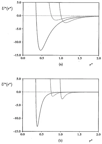
parametrized for discs, exhibits unrealistic behavior at small r. It is easy to show that, for all arrangements of a pair of molecules, except for the edge-to-edge, the

<j(fij, Ui, Uj) term is less than the particle breath ae and so the potential energy

only tends to infinity at negative, unphysical separations. To correct this unrealistic feature, a modified version of the potential was proposed by Bates and Luckhurst

[48], where the potential is shifted and scaled by 07 rather than <re:

where 07 defines the thickness of the discs [48].

Figure (3.3) shows the distance dependence of the potential energy for both ver sions of discotic Gay-Berne potential. It is clear that the modified version posseses many of the same features as the original one (strong face-to-face attraction,

dis-(3.41)

(54)

CHAPTER 3. COMPUTER SIMULATION TECHNIQUES 43

5.0

0.0

--5.0

--10.0

--15.0

0.0 0.5 1.0 1.5 2.0

(a)

5.0

U*(r*)

o.o

--5.0

-- 10.0

-- 15.0

0.0 0.5 1.0 1.5 2.0

(b) r*

[image:54.612.130.464.108.578.2]

(55)

Chapter 4

Preliminary Results

4.1 M odel Development and Testing

A significant amount of time was spent in the development, testing and modifica tion of an initial MD code with which to conduct some preliminary simulations. The first step was to develop an efficient, bug-free integrator - the central part of MD code. This was achieved by running a series of test NVE (constant energy) sim ulations. Starting from simple systems (pure LJ spheres systems), and moving to more complex (pure discotic, rod-sphere systems, where rotational motions should be considered) total energy conservation was checked. It was found that for both

short times (10 time steps) and long times (few million time steps) the total energy

deviations were within 5 • 10-5 units of energy per particle or 0.003% of the average.

This provides confidence that this central part of the MD code was bug-free and both translational and rotational moves were treated correctly.

The second major stage of code development was to improve its efficiency. As was discussed in a previous chapter, the Verlet neighbour list is an effective method to save computational time in the main force calculation loop. After implementa tion of this technique and performing a series of test simulation runs, results were compared with data obtained with earlier