Discussion Papers in Economics
No. 2000/62
Dynamics of Output Growth, Consumption and Physical Capital
in Two-Sector Models of Endogenous Growth
by
Farhad Nili
Department of Economics and Related Studies University of York
No. 2003/16
Coupon Bond Valuation with a Non-Affine Discount Yield Model
by
November 3, 2003
COUPON BOND VALUATION WITH A NON-AFFINE
DISCOUNT YIELD MODEL
Abstract
I report a closed form for the Laplace transform of the Ahn Gao (1999) discount function and show how it generates closed form solutions for the prices of coupon bonds, including hybrid
fixed/variable rate instruments. In contrast, numerical techniques have to be used to analyse these prices for the standard affine yield specifications. I show that many of the characteristics of the Cox Ingersoll and Ross (1980) solutions extend to this more general specification. The allowance for mean reversion in the Ahn-Gao specification means that the solutions are hypergeometric rather than power functions, but the properties of these functions are nicely established, facilitating qual-itative analysis. The prices of interest rate options can be backed out of these formulae by Laplace inversion, overcoming a major problem with the original Ahn and Gao (1999) valuation approach.
JEL Nos: C6, E21, G11-13.
Key words: Non-affine yield curve; Bond valuation, Laplace transform.
(*) I am indebted to Karim Abadir for help with the derivation of the closed form of the transform and to Marco Realdon for extensive discussions on this material. William Perraudin, Steven Satchell and John Knight also provided helpful advice.
Peter D. Spencer University of York
1
Introduction
The theory of the yield curve has developed beyond all recognition over the last quarter of a century. Vasicek (1977) developed the first model of a bond market in which arbitrage
opportunities between different securities were absent. A more realistic specification, which allowed the volatility of the spot rate to be state-dependent, was developed by Cox Ingersoll and Ross (CIR, 1985). These models are easily manipulated and have beenfitted to a wide
range of nominal and real bond price data sets. They yield closed form solutions for the prices of interest rate options and other derivatives. They have been extensively used by practitioners for pricing interest rate derivatives and other securities (Rebonato (1998)).
These two models are encompassed by the specification of Duffie and Kan (1996) in which the yield to maturity is an affine function of the spot rate. However, studies of the spot rate dynamics have raised serious doubts about the spot rate diffusion underpinning this affine yield specification (Chan, Karyoli, Longstaff and Sanders (1992), Aït-Sahalia (1996), Conley et al (1997), Stanton (1997), Jiang and Knight (1997) and Nowman (1999)). The inconsistency between the assumptions of the affine yield model and the empirical dynamics of the spot rate has been emphasised by many others, including Campbell et al (1996) and Ahn and Gao (1999).
These doubts have stimulated the development of non-affine models that better reflect the empirical characteristics of the spot rate process. Foremost amongst these is the specification of Ahn and Gao (1999). They obtain a hypergeometric solution for the price of a default free discount bond under the assumption that the elasticity of the variance is 3, consistent
with the standard empirical result for the US markets. The resulting yield curve is concave rather than linear in the spot rate and provides a better explanation of the yield curve (and, as the earlier studies showed, the spot rate) than the affine model does.
Ahn and Gao (1999) conclude their paper by suggesting that their model could be used for the valuation of caps and floors and other hybrid bond prices. However, there has been
very little progress in this area since the seminal paper of CIR (1980). The lack of closed form solutions for non-zero coupon bond prices in the standard affine yield specifications been a major obstacle. What little work there is has relied heavily upon numerical techniques (Ramaswamy and Sundaresan (1986), Buttler (1995) and Cathcart (2000)). Moreover, as Ahn and Gao (1999) note, their model is at a technical disadvantage to the affine models because the transition densities of the spot rate under the forward neutral measure does not exist in closed form. This means that the expressions for interest rate and bond options are not available in closed form. They suggest the use of Monte Carlo simulations, which are notoriously slow and practically impossible to use in valuing securities with path dependent prices (like barrier options).
However, this paper shows that the Ahn Gao (1999) specification actually has an im-portant technical advantage over the affine models: the Laplace transform of the discount function exists in closed form. This is a characteristic that it shares with the original CIR (1980) specification, which is a special case of Ahn Gao (1999), without mean reversion in the spot rate. The Laplace transform precipitates closed form and quasi-closed form solutions for non-zero coupon bond prices, including hybrids with caps and floors, allowing these prices
to be obtained without relying unduly upon numerical techniques. Qualitatively, many of the characteristics of the CIR (1980) solutions extend to this more general specification. The allowance for mean reversion in the Ahn Gao (1999) model means that the solutions are hypergeometric rather than power functions, but the properties of these functions are well established. They allow non-zero coupon bond prices to be analysed qualitatively, just like the hypergeometric discount prices of the original paper. This analysis extends CIR (1980) and supports their conjecture that their qualitative results would extend to a more general model. These results allow accurate and instant pricing of derivatives like interest rate options, side-stepping the transition density problem identified by Ahn and Gao.
The plan of the paper is as follows. The next section provides a brief description of the Laplace transform and its properties and demonstrates its use as a tool for coupon bond and annuity valuation. Section 3 is supported by appendix 1 and provides a brief summary of the Ahn Gao (1999) model and its assumptions, deriving the closed form for the Laplace transform and then applying the earlier results. Section 4 provides a general pricing lemma that can be used tofind the Laplace transform of a wide variety of bond prices
(including path dependent securities). Closed form solutions for the prices of perpetuities follow immediately. This section values fixed and floating rate annuities and the associated
swap rates; hybrid bonds and interest rate options. Section 5 illustrates the way that the model can be used to price path-dependent securities. The emphasis is on the pricing of default free securities and the technical discussion of defaultable bonds is relegated to appendix 2. The conclusion offers a summary of the main findings and argues that this
coupon pricing framework provides a more appropriate way of modelling the term structure econometrically than the existing approach, which is tofit the discount function to estimates
of discount prices obtained indirectly from coupon bond prices.
2
The Laplace transform and coupon bond valuation
The Laplace transform is a standard mathematical tool, with important financial
applica-tions. In this section I show how it can be used to price a range of non-zero coupon bonds given a specification of the discount function. The results are generic, but are illustrated in the later sections using the Ahn Gao (1999) discount function.
2.1
The valuation of zero-coupon bonds
Consider the general diffusion:
Assumption A1: Let r represent the short term riskless interest rate and let its dynamics under the risk-neutral probability measure be specified by the diffusion:
dr =ζ(r)dt+ξ(r)dw (1)
where wt is a standard Weiner process. Also, make the standard assumptions:
Assumption A2: The financial markets are in continuous transactions-costless equilib-rium.
Standard arbitrage pricing arguments can be used to show that under these assumptions the evolution of any default-free zero-coupon1 instrument V(τ, r) is determined by the
homogeneous partial differential equation (PDE): 1
2ξ(r)
2∂2V /∂r2+ζ(r)∂V /∂r
−∂V /∂τ =rV (2)
whereτ represents time to the terminal maturity date. If the bond pays a coupon of cthen this is added to the left hand side of the PDE (which shows the rate of return expected under the risk neutral measure), making this a non-homogeneous PDE. A similar equation results if the issuer can default and this event is a counting or jump process with intensity (under the risk-neutral measure) ofλ:
wλ+1 2ξ(r)
2∂2V /∂r2+ζ(r)∂V /∂r
−∂V /∂τ = (r+λ)V (3)
where w is the recovery value in default (Dai and Singleton (2003)). As Dai and Singleton note, even though this prices a zero-coupon bond, the possibility of early recovery in the event of default effectively introduces a continuous dividend or coupon of c = wλ. These payments must be discounted at the default-risk adjusted rate(r+λ).Payments from bonds with sinking funds that redeem bonds at face value F and intensity λ are valued by this equation if wλ is replaced by the face value (Goldstein, Ju and Leland (1997)). In this paper, I focus on the valuation of default free instruments using (2). However, appendix 2 shows that the results extend readily to a reduced form default model. Section 5 discusses the way in which the model could be developed to provide a structural model of default risk.
1 In this paper I use the term ‘zero coupon bond’ to describe any security that offers a single future
payment. This includes bonds that offerfloating rate or hybrid payments as well as discount bonds that offer a unit payment.
The valuation PDEs (2) and (3) are solved together with the two boundary conditions:
V(τ; 0) =f inite; (4)
lim
r→∞V(τ;r) = 0;τ >0. (5) and an initial value condition that depends on the specification of the terminal payment. In the case of the generic instrument offering the single payment p(τ, rτ) after a time interval
of τ,the initial value condition (7) is:
V(0;r0) =p(0, r0). (6)
In the case of a standard discount bond with value D(τ;r)paying $1 at maturity we set:
V(0;r0) =D(0;r0) = 1. (7) Differentiating the negative of the log of this price with respect to the maturity then gives the forward interest rate: G(τ;r):
G(τ;r) =−∂logD(τ, r)
∂τ . (8)
Alternatively, the initial condition p(0, r0) = r0 generates the cash value of aτ period spot interest receipt traded in the FRN market which I denote by R(τ;r). In an arbitrage free market this must be equal to the present value G(τ;r)D(τ;r) of the τ period forward rate (8) :
R(τ;r) =G(τ;r)D(τ;r) =−∂D(τ, r)
(Cox, Ingersoll and Ross, (1981), Rebonato (1998))2 . Similarly for a caplet or interest
rate option that pays the excess of the spot rate over a strike rate ¯r (if positive) we set: p(0, r0) = max(r0 − ¯r,0) with value J(¯r,ρ;r). The second column of Table 1 shows the notation used to represent these one-offpayment structures and the other columns show the associated bond prices.
I now show how the real Laplace transform of the discount function can be used to price a range of non-zero coupon bonds. I follow Cathcart (2000) and suppose:
Assumption A4: Coupons are default free and paid continuously. There are no taxes, and:
Assumption A5: The discount bond market is complete: it is possible to buy or sell discount bonds of any maturity3 .
2.2
The Laplace transform
Suppose that the price structure V(τ;r) is a locally integrable function defined on [0,∞) which satisfies the condition |V(τ;r)eat
| ≤ M for all t ∈ [0,∞) for some real a. Then the Laplace transformLρ of V(τ;r), denoted by L(ρ;r) is defined as:
L(ρ;r) =Lρ{V(τ;r)}=
Z ∞ 0
e−ρτV(τ;r)dτ; . (10)
2 That is because I can secure a future payment of rby enter into a forward contract to pay G(τ;r) at
settlement,financing this by buying a discount bond payingG(τ;r)at that time, but costingG(¯r,τ;r)D(τ, r) today. Alternatively I can simply use the FRN market to buy for cash now. Absent arbitrage, these costs must be identical.
3 This is not particularly restrictive because in an N−factor model a bond of any maturity can be
forρ∈C, where C denotes the complex numbers. This transform is useful in solving partial differential equations (Doetsch, (1974)), including those that arise in hybrid valuation prob-lems (Cathcart (2000)). That is because, multiplying (2) by the factor e−ρτ;and integrating
over [0,∞) reduces this to an ordinary differential equation (ODE) for L(ρ, r):
p(0, r0) = (r+ρ)L(ρ, r)−ζ(r)∂L(ρ, r)/∂r− 1 2ξ(r)
2∂2L(ρ, r)/∂r2 (11)
where the Laplace transform of ∂V /∂τ is integrated using:
Lρ[∂V(τ;r)/∂τ] = Z ∞ 0 e−ρτ[∂V(η;r)/∂η]η=τdτ (12) = Z ∞ 0 ρe−ρτV(τ;r)dτ+ [e−ρτV(τ;r)]∞0 = ρL(ρ;r) −p(0, r0) (using (6) and (10)).
It follows that any representation of the integral (10) for a given price structure V(τ;r) is a particular solution of (11) for the associated payment structurep(0, r0).For example, for the fixed rate structure, with V(τ;r) = D(τ;r), the transform L(ρ;r) = P(ρ;r) (see table
1) is a particular solution to (11) for p(0, r0) = 1. Alternatively, putting V(τ;r) =R(τ;r)in (10) we see thatL(ρ;r) =F(ρ;r) and is a particular solution of (11) withp(0, r0) =r0.
2.3
The real Laplace transform as a perpetuity price
If the Laplace parameterρ is real then the Laplace transform is often of direct interest. To take a well known example, the real Laplace transform of a probability density function gives the moment generating function. Gourieroux et al (2003) provide other financial
time of the single payment price structureV(τ;r)multiplied bye−ρτ. It therefore shows the
cost of acquiring a portfolio that yields a continuous income streame−ρτp(τ, r
τ);τ >0.This
income stream lasts for ever, but decays (or for negative values of this parameter, grows) at the rate ρ as maturity τ increases. In other words, L(ρ;r) is the value of a portfolio generating the same income stream as a perpetual bond, and under A2 and A3 must have the same value as a perpetuity generating the same income stream.
For example, with V(τ;r) = D(τ;r); then L(ρ;r) = P(ρ;r) and shows the cost of acquiring a portfolio of discount bonds that yields a continuous income stream e−ρτ;τ >0.
Absent arbitrage, this must equal the price of a perpetuity with the same payment structure. If ρis set to zero we get the price of a standard fixed coupon perpetuity:
Definition 1 A standard fixed interest rate perpetuity provides the income stream:
p(τ;rτ) = 1; τ ≥0 (13)
and under assumptions A1-5 has the value P(0;r) =R0∞D(τ;r)dτ.
The Laplace transform of the floating rate price structure F(ρ;r) follows directly from
that of the fixed rate structure P(ρ;r). Putting V(τ;r) = R(τ;r) in (10); substituting (9);
and using (12) with p(0, r0) = 1 and L(ρ;r) =P(ρ;r) :
F(ρ;r) = Z ∞ 0 e−ρτR(τ;r)dτ (14) = − Z ∞ 0 e−ρτ[∂D(η;r)/∂η]η=τdτ (15) = 1−ρP(ρ;r) (16)
Hypergeometric formulae P(ρ;r)for and hence F(ρ;r) in the Ahn Gao (199) model are reported in section 3.
2.4
Valuing redeemable bonds and annuities
Once the basic solutions forP(ρ, r)andF(ρ;r)have been found, standard theorems for the Laplace transform can be used to value annuities, redeemable coupon bonds, swaps, hybrid securities and many other instruments. First, if we take the Laplace inverse L−τ1 of L(ρ;r)
we regenerate the original zero-coupon price structure:
V(τ, r) =L−τ1{L(ρ;r)} (17) This is useful when we have a closed form solution for L but not forV , as in the case of a cap for example, analysed in section 4.
A second formula can be used to calculate the price of annuities and coupon bonds of finite maturity. Consider the annuitised value of the generic payment stream p(τ, rτ),
m≥τ ≥0:
N(m, r) = Z m
0
V(τ;r)dτ. (18)
A basic theorem (Theorem 23.5, Bronson (1973)) allows us to write the Laplace transform
of this price as:
Lρ{N(m, r)}=Lρ{
Z m 0
V(τ;r)dτ}=Lρ{V(τ;r)}/ρ=L(ρ;r)/ρ (19)
allowing the annuitised value (18) to be recovered as:
This formula can be used to value standard fixed coupon annuities, floating rate equivalents
and swap rates:
Definition 2 A standard m− period fixed interest annuity provides the income stream:
p(τ;r) = 1; m≥τ ≥0 = 0;τ > m.
and under A1-5 has present value:
A(m;r) = Z m
0
D(τ;r)dτ =L−m1{P(ρ;r)}/ρ}. (21)
The price of a standardm−maturity bond with afixed coupon ofcand redemption value
of unity follows immediately as: D(m;r) +cA(m;r) =L−1
m {P(ρ;r)(1 +c/ρ)}.
Now consider the value of a floating rate annuity (or the floating rate leg of a swap).
Direct integration of (9) gives the standard valuation 1−D(m;r):
Definition 3 A standard m− period floating rate annuity provides the income stream:
p(τ;r) = r; m≥τ ≥0 (22)
= 0;τ > m. (23)
and under A1-5 has present value:
Z m 0
R(τ;r)dτ = 1−D(m;r). (24)
Adding the value of a unit redemption payment gives a value of unity for a straight FRN (CIR (1980).
The m−period fixed for floating swap rate s(m, r) is defined as the coupon that brings
the price of a fixed annuity streams(m, r)A(m;r) into equality with this value:
s(m, r) = 1−D(m;r)
2.5
Hybrid
fi
xed/
fl
oating rate valuation
Finally, Cathcart (2000) shows that the Laplace transform with its associated ODE (11) is very useful infixed/floating rate valuation. Because the ODE is time independent, standard
techniques can be used to ensure regularity at this stage (CIR (1980), Dixit (1993)). This approach is particularly useful when we canfind a closed from solution to the ODE (11) but
not the associated PDE (2), as in the case of the hybrid bonds analysed in section 4. The results of this section apply in principle to any arbitrage-free specification of the bond market. However, they can only be implemented analytically when the Laplace trans-form of the discount function exists in closed trans-form as in the model of the next section. A similar example is provided by Spencer (2002). Otherwise, as in the case of the affine yield specifications for example, they have to be implemented using numerical techniques such as those used by Cathcart (2000). In the case of the Ahn-Gao (200) specification, the closed form for the Laplace transform neatly offsets the absence of one for the transition density under the forward neutral measure, as Table 2 indicates. In addition it greatly facilitates the valuation of fixed/floating rate hybrids.
3
A non-a
ffi
ne model of the yield curve
In this section I report the Laplace transform of the Ahn-Gao discount function and use it to illustrate the results of the previous section. The formula is derived in appendix 1. Following Ahn and Gao (1999)4 I specialise (1) to:
4 In developing their model, Ahn and Gao identify the price of risk explicitly and derive the risk premium
Assumption A10:
dr =κ(θ−r)rdt+σr3/2dw (26)
where: θ,κ ≥0; σ>0.
The well-known perpetuity pricing model of CIR (1980) is a special case of this model with κ= 0. Ahn and Gao note that the inverse of the spot rate obeys a CIR (1985) square root volatility process. Reflecting this observation , its conditional distribution is non-central χ2. They show that the expected value ofr
τ conditional on r0,τ ≥0 is: E{rτ|r0} = αe−uM(q, q+ 1, u)/q (27) where : α= 2κθ σ2(1−e−κθτ);u= e−κθτ r0 ;q= 2(κ+σ 2) σ2 −1 and where M(a, b, z) =1F1 (a, b, z)is Kummer’s hypergeometric function.
Under (26), (2) specialises to:
1 2σ
2
r3∂2V /∂r2+κ(θ−r)r∂V /∂r+∂V /∂τ =rV (28) Ahn and Gao (1999) show that under this assumption, the regular solution of (28); (4); (5) and (7) for the discount price is:
D(τ;r) = Γ(β−γ) Γ(β) M(γ,β,−x)x γ (29) where : x= 2κθ σ2(eκθτ −1)r; (30) γ = 1 σ2[ q φ2 + 2σ2−φ]>0; (31) However in estimating the empirical model reported in table 6 they use the risk-neutral
β = 2κ
σ2 + 2(1 +γ)>0; (32)
φ = κ+σ2/2. (33)
They use the properties of this function to demonstrate that the yield to maturity at any point on the curve is a concave function of the spot rate.
3.1
The Laplace transform of the discount function
Substituting the discount price structure V(τ;r) = D(τ;r) from (29) into (10) gives the integral representation of the Laplace transform
P(ρ;r) = Γ(β−γ) Γ(β) Z ∞ 0 e−ρτM(γ,β,− µ 2κθ σ2r ¶ /(eκθτ −1)) µ 2κθ σ2r ¶γ (eκθτ −1)−γdτ. (34) A hypergeometric representation is given by the lemma:
Lemma 1: The Laplace transform of the discount function (29) can be represented as:
P(ρ;r) = αz2F2([1 +ρ/κθ,1],[2−γ,1 +β−γ], z) +d1(ρ)zγM(γ+ρ/κθ;β;z) where : α= (κθ(1−γ)(β−γ))−1;z = 2κθ rσ2; d1(ρ) = Γ(ρ/κθ+γ)Γ(1−γ)Γ(β−γ) κθΓ(1 +ρ/κθ)Γ(β) . (35)
Proof: See appendix.
The Laplace transformF(ρ, r)of thefloating rate payment structure follows immediately
by substituting (35) into (14):
F(ρ;r) = 1−ραz2F2([1 +ρ/κθ,1],[2−γ,1 +β−γ], z)−d2(ρ)zγM(γ+ρ/κθ;β;z) where : d2(ρ) =
Γ(ρ/κθ+γ)Γ(1−γ)Γ(β−γ)
The price of a standard fixed interest perpetuity is obtained by settingρ to zero:
P(0, r) =αz2F2([1,1],[2−γ,1 +β−γ], z)−
Γ(1−γ)Γ(β−γ)Γ(γ) κθΓ(β) z
γM(γ;β;z).
while annuity and swap rates follow by substituting (35) into (21) and (25).
3.2
Pricing hybrid bonds
These solutions can be used to analyse the prices of hybrid instruments that offer either fixed orfloating rate payments, conditional on the value of the spot rate. I use the ODE for
the Laplace transform of the zero coupon price structure because this is time-independent like that for the perpetuity ODE in CIR (1980). As in that paper, I divide the domain of the spot rate up into segments over which fixed orfloating coupon payments are made and use
particular solutions that are valid over these different segments. This procedure gives the Laplace transform of the hybrid zero coupon price structure, which may be interpreted as a general type of perpetual. Setting ρ to zero again gives a standard perpetual, as analysed by CIR (1980). The prices of annuities, caplets and other interest rate options follow by Laplace inversion of the resulting price formulae using (17) or (20).
Under A1,0 the ODE (11) specialises to:
p(0, r0) = (r+ρ)L(ρ, r)−κr(θ−r)∂L(ρ, r)/∂r− 1 2r
3σ2∂2L(ρ, r)/∂r2 (37)
Recall thatP(ρ, r)as defined in (35) is a particular solution to this equation withp(0, r0) = 15.Similarly,p(0, r
0) =r0 in (36) gives an ODE for the Laplace transform of thefloating rate
5 Withρ= 0we obtain the standard perpetuity valuation ODE (equation (17) in CIR (1980)). This states
that the unit coupon plus the expected capital gain (shown in curly brackets) must equal the risk-adjusted cost of carry rP.
price structure that is obeyed byF(ρ, r).Thus we have particular solutions for simplefixed
andfloating rate payments. Trivially, L(ρ, r) = 0 is a particular solution for p(0, r0) = 0.
These three solutions form the building blocks of the hybrid bond valuation model that is developed in the remaining sections. Solutions for L(ρ, r) can be derived by setting p(0, r0) equal to 0,1 orr0 over different spot rate intervals, and then solving (37) using 0, P, or F respectively as particular solutions. Complementary solutions to (37) are added appropri-ately to ensure continuity and satisfy boundary conditions. These solutions are derived in appendix 1. They are more complicated than the simple power functions identified by CIR (1980), reflecting Ahn-Gao’s allowance for mean reversion. They are of hypergeometric type, resembling those of the Cathcart (i.e. CIR(1985)) specification. However, unlike Cathcart, I have a set of particular solutions in closed form and can impose the appropriate boundary conditions analytically using the asymptotic properties of the hypergeometric function6 .
The basic result is stated as a lemma:
Lemma 2: If Bp(ρ;r) is a particular solution to (37) over the interest rate segment
¯r >r > r then the general solution over this segment is:
B(ρ;r) = Bp(ρ;r) +c1B1(ρ;r) +c2B2(ρ;r);where: (38) B1(ρ;r) = zγM(γ+ρ/κθ;β;z); (39)
B2(ρ;r) = zγU(γ+ρ/κθ;β;z); (40)
6 In her CIR (1985)-based model, the particular solution is an integral of a product of hypergeometric
functions that has to be integrated numerically. The boundary condition corresponding to (56) also has to be imposed numerically. Finally, to derive annuity prices, she performs a numerical Laplace inversion. The only numerical technique used in this paper is Laplace inversion, where I employ the same algorithm as she does.
and where c1 and c2 are arbitrary constants, to be determined by the appropriate boundary
conditions. U(a;b;cr)is Tricomi’s hypergeometric function, defined and discussed in (Slater (1960), (1966)).
Proof: See appendix.
The asymptotic properties of hypergeometric functions are well established and I draw upon them heavily in appendix 1. Analytical formulae for the derivatives of the functions can be used to show that:
[∂B1(ρ;r) ∂r ]¯r = − γ+ρ/κθ βr¯ z¯ γ+1M(1 +γ+ρ/κθ; 1 +β; ¯z) −γz¯γM(γ+ρ/κθ;β; ¯z)/¯r ≤ 0 (41) [∂B2(ρ;r) ∂r ]¯r = (γ+ρ/κθ)¯z γ+1U(1 +γ +ρ/κθ; 1 +β; ¯z)/¯r −γz¯γU(γ+ρ/κθ;β; ¯z)/¯r Similarly, the derivatives of the particular solutions P(ρ;r) andF(ρ;r) = 1−ρP(ρ;r) can be obtained from: [∂P(ρ;r) ∂r ]r¯ = α[¯z2F2([1 +ρ/κθ,1],[2−γ,1 +β−γ],z)¯¯ r −2 (42) −z¯2 ( 2 +ρ/κθ (3−γ)(2 +β−γ))2F2([2 +ρ/κθ,2],[3−γ,2 +β−γ],z)]¯ −d1(ρ)[ ∂B1(ρ;r) ∂r ]¯r. The sign restriction in (41) is important for extending the CIR (1980) qualitative analysis
to the mean reverting model. It follows from (31); (32) and the property thatM(a, b;x)≥0 when a, b≥0; (Slater (1960)).
4
Illustrative hybrid payment structures
Following CIR (1980) and Cathcart (2000), the values of hybrid fixed-floating payment
structures are built up by using the alternative particular solutions to generate fixed or
floating payments over different interest rate segments, using the complementary solutions
to ensure continuity and satisfy boundary solutions. This analysis is set out in appendix 1. This section reports some basic price formulae that can be used to value more complex instruments. The basic building block is the value of an interest rate ‘cap’.
Issuers of FRNs often hedge themselves against high interest rates by buying insurance in the form of ‘caps’. These instruments pay the difference between the spot rate and a ceiling ¯
r (if positive) over some future time interval. They effectively convert an FRN liability into a capped FRN, which pays a floating rate of r up to some ceiling r,¯ which is then capped
out at that rate (Rebonato (1998)). They are viewed as a series or stream of ‘caplets’ or interest rate options each of which paysrτ −r¯if positive after the elapse of time τ :
Definition 4 A standard τ− period caplet has price J(¯r,τ;r) and yields a payment after
time τ of:
p(τ;r) = max(rτ −r,¯ 0) (43)
Under (1) these values follow from:
Proposition 1 The Laplace transform of the caplet price structureJ(¯r,τ;r)under
assump-tion (26) is:
Q(¯r,ρ;r) = 1−[¯r+ρ]P(ρ;r) +a1(¯r,ρ)B1(ρ;r); ¯r≥r≥0; (44) =c2(¯r,ρ)B2(ρ;r); r >r.¯
where c2 and a1 follow from the value matching and smooth pasting conditions as: a1 = ([¯r+ρ]P(ρ;r)−1)[∂B2(ρ;r)/∂r]r¯−[¯r+ρ]B2(ρ; ¯r)[∂P(ρ;r)/∂r]r¯ WB(ρ; ¯r) (45) c2 = ([¯r+ρ]P(ρ;r)−1)[∂B1(ρ;r)/∂r]r¯−[¯r+ρ]B1(ρ; ¯r)[∂P(ρ;r)/∂r]r¯ WB(ρ; ¯r) (46)
where the derivatives are defined in (41) to (42) and where WB(r) is the Wronskian, derived from (54) as: WB(ρ;r) =B1(ρ;r)[ ∂B2(ρ;r) ∂r ]¯r−B2(ρ;r)[ ∂B1(ρ;r) ∂r ]r¯ =−Γ(β)(2κθ rσ2) 2γ er2κθσ2/Γ(γ+q/κθ)<0.
Proof: See Appendix.
The price of the capletJ(¯r,τ;r)follows by substituting L(ρ;r) =Q(¯r,ρ;r)into (17) and the priceC(¯r, m;r)of a standardm−period cap follows by putting this in (20). Subtracting the latter from the baseline FRN value of unity shows the price of anm−period FRN with an interest rate ceiling at ¯r .
Structures (13), (43) and their associated values form the building blocks of the hybrid valuation model. These follow in a straightforward way from standard relationships. For example, the value of a floorlet or interest rate put option follows immediately from the
value of the caplet and put-call parity. This instrument offers a single payment defined by: p(τ;r) = max(r−rτ,0) = max(rτ − r,0) + r−rτ. Note that the first component is
furnished by an r-caplet, the second by a discount bond of face value r and the third by selling an interest rate forward. Thus the present value of the floorlet is: J(r,τ;r) + (r
− G(τ, r))D(τ, r). It follows that the cost of an m−period ‘floor’ providing the annuitised payment streammax(r−rτ,0);m ≥τ ≥0is: C(r, m;r) +rA(m, r)−(1−D(τ, r)). Finally,
adding the unit value of a standard FRN gives the value of an m−period FRN with an interest ratefloor atr:C(r, m;r) +rA(m, r) +D(τ, r)7.
5 10 15 20 maturity 0.02 0.04 0.06 0.08 price
Future Forward Option
Figure 1: Prices of futures (H(τ; 0.04)), forwards (G(τ; 0.04)) and 5% call options (G(0.05,τ; 0.04)) as a function of maturity (r= 4%).
The prices for these various interest rate options can in turn be used to price Forward Rate Agreements that are negotiated in advance, but settled at maturity. As with any forward price, a forward option priceG(¯r,τ;r)is derived from the cash equivalent (Rebonato (1998)) by dividing by D(τ, r) : G(¯r,τ;r) = J(¯r,τ;r)/D(τ, r) 8 . Obviously if the strike price is set to zero, the forward option must cost the same as the standard forward price : G(0,τ;r) = G(τ;r). Similarly the value of a forward put option isJ(r,τ;r)/D(τ, r) + (r+ G(τ, r));.where r is the strike rate.
Figure 1 shows some basic results obtained using the risk-neutral parameter estimates on the interest payments of a floater can be constructed by using combinations of these instruments. For example, an m−period FRN offering a rate with bounds at (¯r, r) is constructed by subtracting the value of the capC(¯r,τ;r)from the floored FRN price: C(r, m;r) +rA(m, r)−D(τ, r)−C(¯r,τ;r).The value of interest rate straddle options can be calculated along similar lines using the prices for put and call options.
8 That is because I can secure a future payment ofp(τ;r) = max(r
τ−r,¯0)either by buying forJ(¯r,τ;r)
cash now, or entering into a forward option to payG(¯r,τ;r)at settlement,financing this today by buying a discount bond payingG(¯r,τ;r)at that time, but costingG(¯r,τ;r)D(τ, r)today. In the absence of arbitrage, these alternatives must cost the same.
provided in Table 6 of Ahn Gao (1999) for the period 1960-1991:θ = 2.060;κ= 0.9801;σ= 1.595. The initial value of the spot rate is set at r0 = 0.04. The interest rate future follows immediately from the standard result that a future is a martingale under the risk-neutral measure, which means that the future is the current expectation under this measure. Substituting these parameter estimates into (27) gives the structure of futures prices shown as the dashed line in the Chart. It may be shown that the maturity asymptote is H∞ = 2κθ/(2κ+σ2) = 0.08 96. Similarly, the forward rate structure follows directly from (8) and is shown as the dotted line in the chart. The asymptote is G∞ = κθγ = 0.07423. The continuous line shows the value of a forward option to receive: max(rτ −0.05,0). This is
calculated as G(0.05,τ; 0.04) = J(0.05,τ; 0.04)/D(τ,0.04); where the numerator is obtained from (44) using the method of Gaussian Quadrature developed by Piessens (1969) and used on a similar problem by Cathcart (2000)9 . Recall that Ahn Gao suggest the use of Monte
Carlo techniques for option pricing, which are an order of magnitude slower.
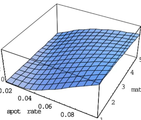
Figure 1 shows that the forward call option price is increasing in the time to expiry, reflecting the increasing likelihood that the interest rate, starting at 4%, will move above the strike of 5%. This effect obviously depends upon the initial interest rate, as shown in Figure 2. This shows the forward call priceG(0.05,τ;r) =J(0.05,τ;r)/D(τ, r)as a function of the initial value of the spot rate (r) as well as maturity (τ). With an initial interest rate of 10%, the call is a decreasing function of maturity, since a longer time interval makes it slightly less likely that the call will be exercised.
9 The accuracy of this technique was checked by comparing the results of numerical inversion of (35)
0.02 0.04 0.06 0.08 0.1 spot rate 1 2 3 4 5 maturity 0 0.02 0.04 price 0.02 0.04 0.06 0.08 0.1 spot rate
Figure 2: The price of a forward call option with a 5% strike: G(0.05,τ;r).
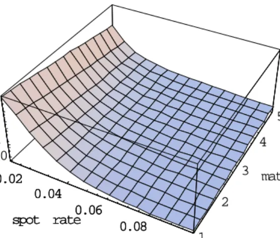
Figure 3 shows the price of the matching forward put option, calculated asG(0.04,τ;r) + 0.04−G(τ;r). This is a decreasing function of time to maturity when the initial interest rate is below 5%, because the passage of time makes exercise less likely. As we would expect, the put option price is a decreasing function of the initial spot rate.
5
Path dependent securities
In the examples used so far, the value of the instrument only depends upon the current state vector(r,τ).As Ahn and Gao (1999) note in the context of bond options, such securities can always be valued faute de mieux using Monte Carlo methods. However, these methods are extremely difficult to use in the case of path dependent securities, where the payoffdepends upon the history of the state variables. Examples include American & barrier options and convertible & callable bonds, wherefinal values depend upon whether particular states have
0.02 0.04 0.06 0.08 0.1 spot rate 1 2 3 4 5 maturity 0 0.01 0.02 0.03 price 0.02 0.04 0.06 0.08 0.1 spot rate
Figure 3: The price of a forward put option with a 5% strike: G(0.04,τ;r) + 0.04−G(τ;r). been attained during the life of the instrument. In practice,finite difference methods are used
to solve the valuation PDE for these securities (Wilmot, (1998)). However, these methods can lead to unacceptable approximation errors: Buttler (1995) analyses the value of a bond that can be called by the issuer on afinite number of dates, comparing the numerical results
with those obtained using the Green’s function (Buttler and Waldvogel, (1996)).
Unfortunately to obtain the Green’s function we again need the transition densities under the forward neutral measure in closed form. Moreover, this approach cannot be employed when the instrument can convert at any time, as in the case of a barrier option for example. However, Cathcart (2000) shows how the Laplace transform handles this pricing problem. This approach is particularly effective in the Ahn Gao (1999) pricing model because (unlike her CIR (1985)-based specification) the particular solutions are available in closed form. I illustrate this point by pricing the bond with the ‘drop lock’ feature analysed by Cathcart
(2000):
Definition 5 A bond with a drop lock feature costs Y(¯r,r, m;ˆ r) and pays the floating rate
r initially, which swaps into thefixed rate ¯r when the spot rate falls to the trigger valuer.ˆ It has a unit redemption payment.
Proposition 2 The price of a redeemable drop lock instrument Y(¯r,ˆr, m;r)under (26) is:
Y(¯r,r, m;ˆ r) = 1 +L−ρ1{[(¯r/ρ+ 1)P(ρ; ˆr)−1/ρ}B1(ρ;r)/B1(ρ; ˆr)};r >rˆ (47) = ¯rL−ρ1{P(ρ; ˆr)/ρ}+V(m,r);ˆ r = ˆr.
In the case of a perpetuity this simplifies to:
Y(¯r,r;ˆ r) = 1 + [rP¯ (0; ˆr)−1 B1(0; ˆr)
]B1(0;r); r >rˆ (48) = ¯rP(0; ˆr);r= ˆr.
Proof: See appendix.
These formulae show that the drop lock feature adds or subtracts from the unit value of a straight FRN depending upon whether the value at conversion is greater than the value of a straight FRN: r¯L−1
ρ {P(ρ; ˆr)/ρ}+V(m,r)ˆ ≶ 1. This premium will be positive if r¯is
high relative torˆ. The sign restriction onB1(ρ;r)in (41) means that the absolute value of the premium (or discount) is a decreasing function of the spot rate. This effect is evident in Figure 4:
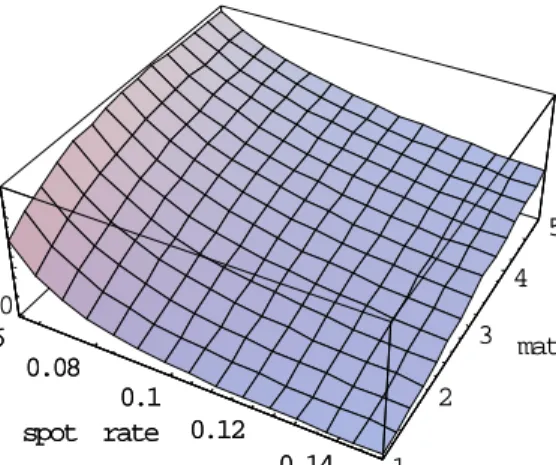
This figure shows the price of a drop-lock FRN that offers afloating rate until the spot
rate falls to 6%. It then offers 6% fixed until redemption. The relatively high value of this
guarantee means that the security trades at a premium to the FRN vanilla value of unity. The figure shows that this premium increases with maturity.
0.06 0.08 0.1 0.12 0.14 spot rate 1 2 3 4 5 maturity 0 0.01 0.02 price 0.06 0.08 0.1 0.12 0.14 spot rate
Figure 4: Price of a drop-lock FRN that locks into 6% fixed.
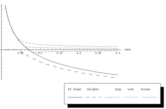
The effect of different lock-in values is shown by figure 5, which shows the prices of
20-year securities. The continuous curve shows the price of a standard 8%fixed rate bond. This
trades at par value when the spot rate is almost 7%. The value of a 20-year instrument with ˆ
r= ¯r= 0.08is shown by the lowest of the three dotted lines and converts into the fixed rate
bond at this rate. It trades at a discount to a vanilla FRN. The central dotted line shows the value of an FRN bond that converts atrˆ= 6%, trading at a premium to the FRN. Note that in each case, the value lines are continuous but exhibit ‘kinks’ as they convert intofixed
rate.
In the case of a convertible, the holder has the once and for all option to swap floating
for fixed payments. As explained in CIR (1980), this ensures that rˆis a point of tangency
between the value curve for the convertible and that for the conversion stock. This solution is illustrated by the highest of the dotted lines in figure 4, which assumes r¯ = 0.08. The
0.05 0.1 0.15 0.2 0.25 0.3 rate 0.6 0.8 1.2 1.4 1.6 price
8% Fixed Callable Drop Lock Prices
Figure 5: 20 year bond prices: The continuous line shows the price of the benchmark 8% fixed coupon security; the dashed line that of an 8% bond callable at par; and the top dotted line that of an FRN convertible into 8%fixed. The other two dotted lines value FRNs that convert into fixed rates of 6% and 8%.
trigger value is calculated as rˆ= 0.041.
Next, consider afixed income bond that has nofinal redemption date, but is ‘callable’ or
redeemable by the issuer. When the spot rate falls to a sufficiently low raterˆ, it will benefit the issuer to call the bond and refinance. As in CIR (1980), the smooth pasting condition that maximises the value of the call option is identical to the conversion condition. This security takes the value of a basic consol but subtracts a weight on the complementary solution B1. The sign restriction onB1(ρ;r) in (41) means that this discount increases monotonically as the spot rate falls to the redemption rate, reflecting the increasing value of the call option to the issuer. The broken line in Figure 5 shows the numerical result obtained using the Ahn
Gao parameters. Again, this assumes ¯r= 0.08 and hence ˆr= 0.041.
Finally, although it is beyond the scope of this paper, the model can be used to develop a structural model of defaultable debt valuation. In these models, bankruptcy occurs when some cashflow or credit indicator falls below a threshold value, which may be endogenous.
The threshold is an endogenous choice variable if the shareholders have the option of issuing additional equity to service debt interest payments. Existing models, including an influential model of bank behaviour by Fries et al (1997), typically assume that the interest rate isfixed.
However, banks and other financial firms are typically exposed to interest rate movements
because they typically borrow at the short end and lending out at the long end of the maturity spectrum. The solution techniques developed in this paper allow this kind of mismatching effect to be analysed by assuming that banks take in variable rate deposits and lend them on in the form of default-freefixed-coupon perpetuities (or mortgages).
6
Conclusion
Despite the advances in modelling the discount yield curve in recent years, there has been little progress in modeling the prices of variable rate instruments since the seminal paper of CIR (1980). What little work there is has relied heavily upon numerical techniques (Ramaswamy and Sundaresan (1986)). The work of Cathcart (2000) uses the theory of the Laplace transform to approach the hybrid valuation problem in the affine CIR (1985) model and represents a big step forward in this area. However she does not obtain these solutions in closed form as I do, but as integrals that have to be integrated numerically. This also
means that she has to impose the boundary conditions numerically.
The closed form for the Laplace transform of the Ahn Gao model provides convenient formulae for the prices of non-zero coupon bonds, including fixed/floating rate hybrids and
bonds with call and conversion features. The theoretical analysis of Cox Ingersoll and Ross (CIR, 1980) can thus be extended to allow for mean reversion and finite maturity. CIR
(1980) admit that their model is a simple one, but they suggest that ‘many of the qualitative properties should carry over to more complex models’. The existence of closed form solutions for these security prices allows this conjecture to be confirmed. I find that many of the
characteristics of the CIR (1980) solutions extend to this more general specification. The allowance for mean reversion in the Ahn Gao (1999) model means that the solutions are hypergeometric rather than power functions, but the properties of these functions are well established, allowing non-zero coupon bond prices to be analysed qualitatively.
The paper provides closed form and quasi closed form solutions for the hybridfixed/floating
structures described by Cathcart (2000) and shows that it is remarkably easy to apply the model to the valuation of caps andfloors, providing the extension suggested by Ahn and Gao
(1999). These results allow accurate and instant pricing of derivatives like interest rate op-tions, overcoming the problem with the forward risk neutral measure identified by Ahn and Gao. The ability of the model to price these instruments arguably provides the bond trader with a more versatile as well as a more realistic alternative to the affine model. These results can be readily extended to other non-affine specifications in which the Laplace transform of the discount function exists in closed form (Spencer (2002)). The model easily lends itself
to other theoretical applications, for example in pricing defaultable debt and convertible & callable bonds.
For the econometrician, these results open the way to direct non-linear regression mod-eling of coupon bond and swap price data. Conventionally, the yield curve is calibrated by fitting formulae for the discount function to indirect estimates of the discount curve. These
are derived by regressing coupon bond price data on variables representing maturity and coupon. This is the approach used by Ahn Gao (1999), who fit (29) to the discount price
data estimated by McCullock and Quon (1992). However the use of a regression estimate as the regressor is problematic and could lead to a spuriously good fit. It might also introduce
measurement error10 11 . Indeed, in their econometric models Ahn Gao replace the spot rate
estimate of McCullock and Quon by a market interest rate, noting that the former contains a large degree of extrapolation error.
Recent work on the term structure has used estimates of the discount function derived from the swap curve. The swap market is now more liquid than the bond markets, providing a better test framework for arbitrage pricing models. However, the swaps market is essentially a coupon bond market and could also be modeled directly using formulae such as (25). All in all, the Ahn Gao discount function and its Laplace transform would seem to offer both academics and practitioners a very useful addition to the bond valuation tool-kit.
10 Tax clientelle and other distortions are also difficult to allow for (Schaefer (1981)).
11 An alternative approach would be to model data from the US Treasury Strips curve, which in principle
give a market estimate of discount bond prices. However, these markets are thin and there is evidence that the long end is artificially increased by ultra-long investors seeking duration.
7
Appendix 1
7.1
Proof of lemma 1
This shows how the closed form Laplace transform (35) can be derived from the integral representation (34). First adopt the change of variable:
z = 1/(eλτ −1)⇐⇒τ = ln(1 + 1/z)/λ
and rewrite (34) as:
P(ρ;r) = c γΓ(β −γ) λΓ(β) Z ∞ 0 zγ+ρ/λ−1(1 +z)−(1+ρ/λ)M(γ,β,−cz)dz where : c= µ 2κθ σ2r ¶ ;λ=κθ
The integral in this expression has a closed form. This is reported (as Equation 14, page 260, volume 3) by Prudnikov et al (1985). This may be derived as follows. First substitute the standard integral representation of the Kummer hypergeometric function to get (49). Changing the order of integration then allows us to use the integral representation of the Kummer hypergeometric function to get (50). Then (51) represents this in terms of Kum-mer functions. These integral representations are shown as 13.1.36; 13.2.5 and 13.1.3 in Abramovitz and Steigun, (1965).
P(ρ;r) = c γ λΓ(γ) Z ∞ 0 zρ/λ+γ−1(1 +z)−(1+ρ/λ)[ Z 1 0 e−czttγ−1(1−t)β−γ−1dt]dz (49) = c γ λΓ(γ) Z 1 0 tγ−1(1−t)β−γ−1[ Z ∞ 0 zρ/λ+γ−1(1 +z)−(1+ρ/λ)e−cztdz]dt = cγΓ(ρ/λ+γ) λΓ(γ) Z 1 0 tγ−1(1−t)β−γ−1J(γ+ρ/λ,γ;ct)dt (50)
= cγΓ(ρ/λ+γ) λΓ(γ) Z 1 0 tγ−1(1−t)β−γ−1[(ct) 1−γΓ(γ −1)M(1 +ρ/λ,2−γ;ct) Γ(γ+ρ/λ) (51) +Γ(1−γ)M(γ+ρ/λ,γ;−cz) Γ(1 +ρ/λ) ]dt.
Finally, series representation of these two Kummer functions (Abramovitz and Steigun, (1965): 13.1.2) and term by term integration of the resulting Beta functions (noting that β >γ)gives (35) and completes the proof:
P(ρ;r) = cγΓ(ρ/λ+γ) λΓ(γ) Z 1 0 tγ−1(1−t)β−γ−1[(ct) 1−γΓ(γ −1) Γ(γ +ρ/λ) ∞ X n=0 (1 +ρ/λ)n(ct)n n!(2−γ)n + Γ(1−γ) Γ(1 +ρ/λ) ∞ X n=0 (γ+ρ/λ)n(ct)ndt n!(γ)n ] = 1 λΓ(γ)[cΓ(γ−1) ∞ X n=0 (1 +ρ/λ)ncn R1 0 t n(1 −t)β−γ−1dt n!(2−γ)n +Γ(ρ/λ+γ)Γ(1−γ)c γ Γ(1 +ρ/λ) ∞ X n=0 (γ+ρ/λ)ncn R1 0 t n+γ−1(1 −t)β−γ−1dt n!(γ)n ] = cΓ(γ−1) λΓ(γ) ∞ X n=0 (1 +ρ/λ)nΓ(n+ 1)Γ(β−γ)cn n!(2−γ)nΓ(1 +β+n−γ) +Γ(ρ/λ+γ)Γ(1−γ)c γ λΓ(γ)Γ(1 +ρ/λ) ∞ X n=0 (γ+ρ/λ)nΓ(n+γ)Γ(β−γ)cn n!(γ)nΓ(β+n) = c λ(γ−1)(β−γ) ∞ X n=0 (1 +ρ/λ)n(1)ncn n!(2−γ)n(1 +β−γ)n +Γ(ρ/λ+γ)Γ(1−γ)Γ(β−γ)c γ λΓ(1 +ρ/λ)Γ(β) ∞ X n=0 (γ+ρ/λ)ncn n!(β)n = αz 2F2[(1 +ρ/κθ,1); (2−γ,1 +β−γ), z] +d1zγM(γ+ρ/κθ,β, z)
7.2
Proof of Lemma 2
Lemma 2 follows directly from the fundamental theorem of linear differential equations, which states that any solution can be expressed as the sum of any particular solution and a weighted sum of its complementary solutions (Simmons (1972), Chapter 3, Theorem B). These are the solutions to the homogeneous analogue of (37) :
0 = (r+ρ)L(ρ, r) + [r2κ−rκθ]∂L(ρ, r)/∂r−1 2r
3σ2∂2L(ρ, r)/∂r2 (52)
Adopting the changes of variable:
r= 2κθ/σ2z; L(ρ, r) = zγY(z(r)) (53)
transforms equation (52) into Kummer’s differential equation (Slater (1960)): 0 =z∂2Y(z)/∂r2+ (β−z)∂Y(z)/∂r−(γ+ρ/κθ)Y(z). The solution set for Kummer’s equation may be written as:
Y(z) = b1Y1(z) +b2Y2(z); where: Y1(z) = M(a;b;z);
Y2(z) = U(a;b, z). a = γ+ρ/κθ;b=β
and where b1 and b2 are arbitrary coefficients. M(a, b, z) is Kummer’s confluent hypergeo-metric function, andU(a, b, z) is Tricomi’s hypergeometric function. The Wronskian of this system is (Slater (1960), 13.1.20):
WY =Y1Y20−Y2Y10 =−Γ(b)z−
SubstitutingY1 andY2into (53) gives the solutionsB1 andB2reported in (38) and completes the proof of the lemma.
7.3
Asymptotic behaviour
As noted in section 3, the values of hybrid fixed-floating payment structures are built up
byfinding a particular solution that generates the payments relevant over different interest
rate segments. Then complementary solutions are added to ensure continuity and satisfy boundary conditions. The rest of the appendix shows how the boundary conditions (4) and (5) can be implemented analytically for different types of payment structure using the asymptotic properties of the hypergeometric function. I first take the Laplace transform of
both sides of each inequality to get:
L(ρ; 0) =f inite; (55)
lim
r→∞L(ρ;r) =f inite. (56)
The solutions to the Laplace valuation ODEs must obey these restrictions if the under-lying zero price structures are to obey (4) and (5). First consider the behaviour of these functions at the right boundary. The basic property used in this case is that the 1F1 and 2F2 functions have unit value for z = 0. The basic result follows directly from (39);
lim
r→∞B1(r) = limz→0z
γ
M(a;b, z) = 0 (57)
Also, using (35) and (36):
lim
lim r→∞F(ρ, r) = 1 Then with β >2; 1 +γ−β <0: lim r→∞B2(r) = limz→0z γU(a;b, z) = lim z→0z 1+γ−β = ∞ (58)
(Abramowitz and Stegun (1965),13.5.6).
Turning to the left boundary condition (55), the asymptotic behaviour ofB1 follows from a standard result for the 1F1 function:
lim
r→0B1(r) = limr→0( 2κθ rσ2)
2γ−β−ρ/κθe2rσκθ2Γ(β)/Γ(γ+ρ/κθ) =∞ (59)
(Abramowitz and Stegun (1965),13.1.4). Note that2γ−β−ρ/κθ<0.The behaviourB2asr tends zero andz to to infinity follows from that of the Tricomi function: limz→∞U(a;b, cz) = (cz)−a (Abramowitz and Stegun (1965),13.5.2). Consequently, with a = γ+ρ/κθ > 0, B
2 satisfies (55): lim r→0B2(r) = limr→0( 2κθ rσ2) −γ−ρ/κθ = 0. (60)
7.4
Proof of Proposition 1
Recall that a caplet has the payment structure (43) and pays nothing over the lower interest segment r¯ ≥ r ≥ 0. Thus, we set Bp = 0. The value of the Laplace transform over this range is defined by the homogeneous equation (52) and is given by the set of complementary solutions:
c1B1(ρ;r) +c2B2(ρ;r); ¯r≥r ≥0; (61) To satisfy (55), (59) shows that we need c1 = 0.
At higher interest rates r > ¯r, the caplet yields: (rτ − ¯r). Thus we need to find a
particular solution to (37) withp(0, r) = r−r.¯ The linearity of (37) allows us to build this up as the sum of any particular solution with p(0, r) = r less another one with p(0, r) = ¯r; e.g. : F(ρ;r)−rP¯ (ρ;r).Adding in the complementary functions and simplifying using (14) gives the solution set:
1−[¯r+ρ]P(ρ;r) +a1B1(ρ;r) +a2B2(ρ;r); r >r.¯ (62) In this case (56) and (58) require a2 = 0. The system (61) and (62) is solved given c1 = a2 = 0.
Since the interest rate can pass freely through the switch rate r¯in both directions, we require that the solution and itsfirst derivative are continuous at this point. These conditions
are respectively known as the value matching and smooth pasting conditions (Dixit (1993). Substituting c1 =a2 = 0 into (61) and (62):
1−[¯r+ρ]P(ρ; ¯r) +a1B1(ρ; ¯r) =c2B2(ρ; ¯r) (63)
Differentiating (61) and (62) with respect tor, and equating these derivatives at the switch point :
−[¯r+ρ][∂P(ρ;r)/∂r]r¯+a1[∂B1(ρ;r)/∂r]¯r =c2[∂B2(ρ;r)/∂r]¯r. (64) This is solved together with (63) after substituting r = ¯r to give c2 and a1 as specified in (45) and (46). This completes the proof.
7.5
Proof of Proposition 2
The value Y(¯r,r, m;ˆ r) of the floater with the drop-lock feature is the integral of present
values of future interest receipts X(¯r,r,ˆ τ;r) and the redemption V(τ;r)payment:
Y(¯r,ˆr, m;r) = Z m
0
X(¯r,r,ˆ τ;r)dτ +V(m;r) (65)
As long as interest rates remain above the conversion rate, the instrument paysfloating rate
and so the Laplace transform of the price structure for these interest receipts must obey:
Lρ{X(¯r,ˆr,τ; ˆr)}=F(ρ;r)+a1B1(ρ;r)+a2B2(ρ;r) = 1−ρP(ρ;r)+a1B1(ρ;r)+a2B2(ρ;r); r >r.ˆ (66) Again, the right boundary requires a2 = 0. When the spot rate falls to r,ˆ and conversion takes place the redemption payment is not affected but this floating rate stream is swapped
into thefixed rater.¯ Unlike the two-way switch rate of the previous section,rˆis an absorbing
barrier (Dixit (1993)), so we only use the value matching condition at r= ˆr: Z m 0 X(¯r,r,ˆ τ; ˆr)dτ = ¯r Z m 0 D(τ; ˆr)dτ (67)
Taking the Laplace transform of both sides using (19):
Lρ{
Z m 0
X(¯r,r,ˆ τ; ˆr)dτ} = Lρ{X(¯r,r,ˆ τ; ˆr)}/ρ= ¯rLρ{D(τ; ˆr)}/ρ
⇒ Lρ{X(¯r,r,ˆ τ; ˆr)}= ¯rLρ{D(τ; ˆr)}= ¯rP(ρ; ˆr) (68)
Equating (66) and (68) at r= ˆr gives the value of the undetermined coefficient:
Substituting this back into (66) gives the Laplace transform of the price structure for the interest rate stream:.
Lρ{X(¯r,ˆr,τ;r)}= 1−ρP(ρ;r) + [(¯r+ρ)P(ρ; ˆr)−1]B1(ρ;r)/B1(ρ; ˆr); r > ˆr. (70) If the instrument is a perpetuity as in CIR (1980) then settingρ= 0gives the price directly:
Y(¯r,r, r) =ˆ Z ∞
0
X(¯r,r,ˆ τ;r)dτ =Lρ[X(¯r,ˆr,τ; ˆr)]ρ=0 = 1+[¯rP(0; ˆr)−1]B1(0;r)/B1(0; ˆr); r >r.ˆ (71) For a redeemable we use (65) and (70) to get the Laplace transform of the price:
Lρ{Y(¯r,r, m;ˆ r)}=Lρ{X(¯r,ˆr,τ;r)}/ρ+Lρ{V(τ;r)}= 1/ρ+[(¯r+ρ)P(ρ; ˆr)−1]B1(ρ;r)/ρB1(ρ; ˆr) (72) Laplace inversion then gives the drop lock price shown at (47), which equates with the value of the conversion stock at the trigger point. This completes the proof.
8
Appendix 2: Default risk and premature repayment
This appendix shows how the default free bond price formulae can be modified to allow for default risk, using the observation of Dai and Singleton (2003) that the possibility of early recovery in the event of default effectively introduces a continuous dividend or coupon of c = wλ. This premature payment effect can therefore be evaluated by modifying the argument used to obtain the annuity formula (20). Adding in the value of the possible final
Recall that the price of a defaultable discount bond is determined as the solution to (3); (4); (5) and (7). First, to value the terminal payment, consider the homogeneous analogue of (3) obtained by setting the recovery rate w to zero. Under A10:
1 2r
3σ2∂2V /∂r2+rκ(θ
−r)∂V /∂r−∂V /∂τ = (r+λ)V (73)
It is easy to see that the solution to this equation (with (4); (5) and (7)) ise−λτD(τ, r);where
D(τ, r)is given by (29). This is just the value of a default-free discount bond multiplied by the probability of survival.
Second, to obtain the Laplace transform of the value of early recovery with w > 0, multiply (73) by the factore−ρτ; and integrate over [0,
∞) as for (11) using p(0, r0) = 0: wλ ρ = (r+ρ 0)L(ρ0, r)−rκ(θ−r)∂L(ρ0, r)/∂r− 1 2r 3σ2∂2L(ρ0, r)/∂r2 (74)
whereρ0 = (λ+ρ).This is similar to ((37), now replacingp(0, r0)bywλ andρ byρ0), so the regular solution can be found by appropriate modification of (35):
P D(ρ;r) = wλ ρ αz2F2([1 + (λ+ρ)/κθ,1],[2−γ,1 +β−γ], z) + wλ ρ d1(ρ)z γM(γ+ (λ+ρ)/κθ;β;z) where : α = (κθ(1−γ)(β−γ))−1;z= 2κθ rσ2; d1(ρ) = Γ((λ+ρ)/κθ+γ)Γ(1−γ)Γ(β−γ) κθΓ(1 + (λ+ρ)/κθ)Γ(β) . (75)
The annuitised value of the default payments on a discount bond can then be obtained from (20). Adding in the value of the possible redemption payment gives the total value:
The value of a bond with an early repayment dictated by a sinking fund with intensity λ follows by setting w = 1. Hybrid fixed/floating defaultable zero values can be obtained by
modifying the coupon payment appropriately.
9
References
Abadir, K. (1997): “An Introduction to Hypergeometric Functions for Economists,” Econo-metric Reviews, 18, 287-330.
Abadir, K. (2004): “Explicit Distribution Theory for Simple Time Series”, forthcoming 2004, Wiley, New York.
Abramowitz, M., and I. A. Stegun (1965): Handbook of mathematical functions. Dover Publications, New York.
Ahn, D. H and Gao, B. (1999): ‘A Parametric Model of Term Structure Dynamics’,
Review of Financial Studies, 12, 721-762.
Aït-Sahalia, Y. (1996) “Testing Continuous-Time Models of the Spot Interest Rate” Review of Financial Studies, 9,385-42.
Bronson, R. (1973): “Modern Introductory Differential Equations” Mc Graw-Hill, Lon-don.
Buttler, H-J, (1995): “Evaluation of Callable bonds: Finite Difference Methods, Stability and Accuracy’ Economic Journal, 1056(1), 374-384.
Buttler, H-J, and J. Waldvogel, (1996): “Pricing Callable Bonds by means of Green’s Function,” Mathematical Finance, 6(1),53-88.
Campbell, J. Y., Lo, A. W., and MacKinlay, A.C. (1996): ‘The Econometrics of Financial Markets’ Princeton University Press, Princeton, N.J.
Cathcart, L, (2000): “The Pricing of Floating Rate Instruments”Computational Finance, 1 (4) 221-241.
Chen, K.C., G.A. Karolyi, F.A. Longstaff and A.B. Sanders,: (1992): “An Empirical Comparison of Alternative Models of the Short Term Interest Rate,”The Journal of Finance, 47(3), 1209-1227.
Conley, T. Hansen, L. and Lutmer, E. and Scheinkman, J. (1997): ‘Short-Term Interest Rates as Subordinated Diffusions’ Review of Financial Studies,10, 525-577.
Cox, J.C., J.E. Ingersoll, and S.A. Ross, (1980): “An Analysis of Variable Rate Loan Contracts” The Journal of Finance, 35(2), 389-404.
Cox, J.C., J.E. Ingersoll, and S.A. Ross, (1981): “The relation between forward prices and futures prices,” Journal of Financial Economics, 9, 321-346.
Cox, J. C., J. E. Ingersoll, and S. A. Ross (1985): “A Theory of the Term Structure of Interest Rates,“Econometrica, 53(2), 385-407.
Doetsch, G (1974): ‘Introduction to the Theory and Application of the Laplace transform’ Springer, New York.
Dai, Q. and Singleton, K. (2003): ‘Term Structure Dynamics in Theory and Reality’
Review of Financial Studies, 16 (3), pp 631-678.
Duffie, D. and Kan, R. (1996): ‘A Yield-Factor Model of Interest Rates’ Mathematical Finance, 6, 379-406.
Dixit, A.K.(1993): “The Art of Smooth Pasting” Harwood, Langhorne.
Dixit, A.K. and R.S. Pindyk (1990): Investment under Uncertainty, Princeton.
Dothan, U. (1978): ‘On the Term Structure of Interest Rates’ Journal of Financial Economics, 6, 59-69.
Fries, S. Mella-Barral, P and Perraudin, W. (1997) :‘Optimal Bank Reorganisation and the Fair Pricing of Deposit Guarantees’ Journal of Banking and Finance, (21) 441-468.
Gourieroux, C. Darolles, S. and Jasiak, J (2003) : ‘Structrural Laplace Transforms and Compound Autoregressive Models,’ Working Paper, Crest-Cepremap, Paris.
Goldstein, R., Ju, N., and Leland, H., (1997): “Endogenous Bankruptcy, Restructuring and Dynamic Capital Structure” Working Paper, University of California, Berkeley.
Harrison, M and Kreps, D. (1979): ‘Martingales and Arbitrage in Multiperiod Securities Markets’ Journal of Economic Theory, 20,381-408.
Jiang, G. J and Knight, J. (1997): ‘A Non-Parametric Approach to the Estimation of Diffusion Processes, with an Application to a Short-Term Interest Rate Model’Econometric Theory, 13, 615-645.
McCulloch J.H., and Kwon H-C, (1990) : ‘US Term Structure Data’ manuscript and computer diskettes., Ohio State University, March.
Nowman, B. (1999): ‘Gaussian Estimation of Single-Factor Continuous Time Models of the Term Structure of Interest Rates’ Journal of Finance, Vol. LII, 1695-1706.
Piessens, R. (1969): “New Quadrature Formulas for the Numerical Inversion of the Laplace Transform,” BIT, 9, 351-361.
Prudnikov, A.P., Brychov, Y.A.,and Marichev, O.I, (1985): ‘Integrals and Series’ Volume 3: More Special Functions, Gordon and Breach Science Publishers, New York.
Ramaswamy, K., and S. Sundaresan (1986): “The valuation offloating rate instruments,“
Journal of Financial Economics, 17, 251-272.
Rebonato, R (1998): “Interest rate option models,” Wiley, New York.
Schaefer, S. M. (1981): ‘Measuring a Tax-Specific Term Structure of Interest Rates in the Market for British Government Securities’ The Economic Journal, Vol 91, pp 415-478.
Simmons, G. F. (1972): ‘Differential Equations’ Mc Graw Hill, New York.
Slater, L. J. (1960): “Confluent hypergeometric functions.” Cambridge University Press, Cambridge
Slater, L. J. (1966): “Generalized hypergeometric functions.” Cambridge University Press, Cambridge.
Stanton, R. (1997): ‘A nonparametric Model of Term Structure Dynamics and the Market Price of Interest Rate Risk,”Journal of Finance,52,1973-2002.
Spencer, P.D. (2002):‘Rival Models of the Yield curve: The US Treasury Market
1974-2000’, IFR Discussion Paper 1/2002, Birkbeck College, London:http://www.econ.bbk.ac.uk/wp/fwp/ifr. Vasicek, 0. A. (1977): “An Equilibrium Characterization of the Term Structure,”Journal
of Financial Economics, 5(2), 177-188.
Wilmot, P. (1998): ‘Derivatives: The Theory and Practice of Financial Engineering’ Wiley, New York.
Table 1: The basic valuation building blocks
Type Payment: Zero price: Laplace transform: Perpetuity: Annuity
Generic p(0, r0) V(τ;r) L(ρ;r) = L(0;r) N(ρ;r) = Lρ{V(τ;r)} L−m1{ L(ρ;r) ρ } Fixed 1 D(τ;r) P(ρ;r) P(0;r) A(m, r) Floating r0 R(τ;r) F(ρ;r) F(0;r) 1−D(m;r) Cap max(r0−r,¯ 0) J(¯r,ρ;r) Q(¯r,ρ;r) C(¯r, m;r)
Table 2: Spot rate diffusions and bond valuation
Model: Vasicek (1977) CIR (1985) Ahn Gao (2000)
Gaussian volatility Square root volatility Augmented CIR (1980)
Spot rate:
Diffusion dr=κ(θ−r)dt+σdz κ(θ−r)dt+σr1/2dz κ(θ
−r)r2dt+σr3/2dz
Transition density - actual Gaussian Non-central χ2 Non-centralχ2
- under forward neutral measure Gaussian Non-central χ2 No closed form
Discount yield:
Affine? Yes Yes No