Decomposition-Based Multiobjective Optimization
for Constrained Evolutionary Optimization
Bing-Chuan Wang , Han-Xiong Li , Fellow, IEEE, Qingfu Zhang, Fellow, IEEE,
and Yong Wang , Senior Member, IEEE
Abstract—Pareto dominance-based multiobjective optimization has been successfully applied to constrained evolutionary optimization during the last two decades. However, as another famous multiobjective optimization framework, decomposition-based multiobjective optimization has not received sufficient attention from constrained evolutionary optimization. In this paper, we make use of decomposition-based multiobjective optimization to solve constrained optimization problems (COPs). In our method, first of all, a COP is transformed into a biobjective optimization problem (BOP). Afterward, the trans-formed BOP is decomposed into a number of scalar optimization subproblems. After generating an offspring for each subprob-lem by differential evolution, the weighted sum method is utilized for selection. In addition, to make decomposition-based multiobjective optimization suit the characteristics of constrained evolutionary optimization, weight vectors are elabo-rately adjusted. Moreover, for some extremely complicated COPs, a restart strategy is introduced to help the population jump out of a local optimum in the infeasible region. Extensive exper-iments on three sets of benchmark test functions, namely, 24 test functions from IEEE CEC2006, 36 test functions from IEEE CEC2010, and 56 test functions from IEEE CEC2017, have demonstrated that the proposed method shows better or at least competitive performance against other state-of-the-art methods.
Manuscript received May 15, 2018; revised August 10, 2018; accepted October 2, 2018. This work was supported in part by the General Research Fund Project from Research Grant Council of Hong Kong SAR under Grant CityU 11205615, in part by the Innovation-Driven Plan in Central South University under Grant 2018CX010, in part by the National Natural Science Foundation of China under Grant 61673397 and Grant 61876163, and in part by the Hunan Provincial Natural Science Fund for Distinguished Young Scholars under Grant 2016JJ1018. This paper was recommended by Associate Editor H. R. Karimi. (Corresponding author: Yong Wang.)
B.-C. Wang is with the Department of Systems Engineering and Engineering Management, City University of Hong Kong, Hong Kong (e-mail: [email protected]).
H.-X. Li is with the Department of Systems Engineering and Engineering Management, City University of Hong Kong, Hong Kong, and also with the State Key Laboratory of High Performance Complex Manufacturing, Central South University, Changsha 410083, China (e-mail: [email protected]).
Q. Zhang is with the Department of Computer Science, City University of Hong Kong, Hong Kong, and also with the Shenzhen Research Institute, City University of Hong Kong, Shenzhen, China (e-mail: [email protected]).
Y. Wang is with the School of Information Science and Engineering, Central South University, Changsha 410083, China, and also with the School of Computer Science and Electronic Engineering, University of Essex, Colchester CO4 3SQ, U.K. (e-mail: [email protected]).
This paper has supplementary downloadable material available at http://ieeexplore.ieee.org, provided by the author. It contains analysis and tables related to the main paper. The total file size is 0.2 MB.
Color versions of one or more of the figures in this paper are available online at http://ieeexplore.ieee.org.
Digital Object Identifier 10.1109/TSMC.2018.2876335
Index Terms—Constrained optimization problems (COPs), decomposition, evolutionary algorithms (EAs), multiobjective optimization, Pareto dominance.
I. INTRODUCTION
M
ANY scientific and engineering optimization problemscan be formulated as constrained optimization problems (COPs) [1], [2]. Without loss of generality, a COP can be described as
minimize f(x), x=(x1, . . . ,xD)∈S,Li≤xi≤Ui subject to: gj(x)≤0,j=1, . . . ,l
hj(x)=0,j=l+1, . . . ,m
where f(x)is the objective function, x is the decision vector (a solution or an individual), xi is the ith dimension ofx, D is the number of dimensions, Li and Ui are the lower and upper bounds of xi, respectively, S =
D
i=1[Li,Ui] is the decision space, gj(x)is the jth inequality constraint, l is the number of inequality constraints, hj(x)is the(j−l)th equality constraint, and(m−l)is the number of equality constraints.
For COPs, the degree of constraint violation ofx on the jth constraint is expressed as follows:
Gj(x)= max0,gj(x) , 1≤j≤l max0,|hj(x)| −δ , l+1≤j≤m (1) where δ is a positive tolerance value to relax equality con-straints. Afterward, the degree of constraint violation of x on all constraints is calculated as follows:
G(x)= m j=1 Gj(x) (2)
x is called a feasible solution if G(x) = 0; otherwise, it is called an infeasible solution. The goal of solving a COP is to locate the feasible optimum.
In the community of evolutionary computation, there has been an increasing interest in applying evolutionary algo-rithms (EAs) to solve COPs. In order for EAs to deal with COPs, constraint-handling techniques should be inte-grated. In principle, EAs aim to generate offspring while constraint-handling techniques are in charge of comparing individuals. The last two decades have witnessed the suc-cessful applications of multiobjective optimization to design constraint-handling techniques. In multiobjective optimization-based constraint-handling techniques, a COP is first trans-formed into a multiobjective optimization problem (MOP).
Then, multiobjective optimization techniques are used to com-pare individuals. In this paper, multiobjective optimization-based constraint-handling techniques are briefly classified into three categories: 1) standard multiobjective optimization meth-ods; 2) standard biobjective optimization methmeth-ods; and 3) gen-eralized multiobjective optimization methods. The standard multiobjective optimization methods transform a COP into an MOP with (m+1) objectives, i.e.,(f(x),G1(x), . . . ,Gm(x)). Multiobjective optimization-based constraint-handling tech-niques at the early stage always fall into this category [3], [4]. Under this condition, the transformed MOP always involves more than two objectives. As we know, MOPs with more than two objectives usually exhibit complicated properties. Consequently, the transformed MOP is also very difficult to be tackled as the original COP. In contrast, the standard biobjec-tive optimization methods consider the degree of constraint violation, i.e., G(x), as another objective function in addi-tion to the original objective funcaddi-tion f(x). Interestingly, most of the recent multiobjective optimization-based constraint-handling techniques belong to this category [5]–[9]. Different from the above two categories, the generalized multiobjective optimization methods introduce other additional objective functions or constraints [10], [11].
It can be found that most of the existing multiobjective
optimization-based constraint-handling techniques are
based on Pareto dominance [12], in which Pareto domi-nance is viewed as the criterion to compare individuals. Note, however, that decomposition is another famous multiobjective optimization framework [13]–[15]. Its out-performed performance has been demonstrated in a lot of literature, such as [16]–[18]. Different from Pareto dominance-based multiobjective optimization, decomposition-based multiobjective optimization decomposes an MOP into a set of scalar optimization subproblems, where each subproblem is assigned a weight vector. Afterward, these subproblems are optimized in a collaborative manner. Such a framework exhibits numerous advantages for solving MOPs. By decomposing an MOP into a set of scalar optimization subproblems, every two solutions are comparable. Hence, a certain degree of selection pressure can be guaranteed. Besides, it is well-known that decomposition-based frame-work is more efficient than nondominated sorting [13], [19]. Moreover, by adjusting the weight vectors, search biases can be incorporated. Note that these search biases are crucial when taking advantage of multiobjective optimization to tackle COPs [20], [21]. However, little effort has been devoted to making use of the above advantages of decomposition-based multiobjective optimization for constrained evolutionary optimization.
Motivated by the above considerations, this paper makes an attempt to tailor decomposition-based multiobjective optimization to solve COPs. In our method, a COP is first converted into a biobjective optimization problem (BOP) (f(x),G(x)). Afterward, this BOP is decomposed into NP scalar optimization subproblems. Each individual in the pop-ulation is associated with a subproblem and is evolved along the direction defined by the weight vector of this subprob-lem. After generating an offspring for each subproblem by
differential evolution (DE), the weighted sum method is employed to compare individuals. To make decomposition-based multiobjective optimization suit the properties of COPs, a weight vector adjusting strategy is designed. Furthermore, a restart strategy is introduced to cope with extremely complicated constraints. By the above process, an alterna-tive constrained optimization EA (COEA), i.e., DeCODE, is proposed. Note that DeCODE is different from the constrained decomposition-based multiobjective optimization algorithm introduced in [22]. The algorithm in [22] utilizes constrained optimization to improve the decomposition-based method for multiobjective optimization. On the contrary, DeCODE applies the decomposition-based method to solve COPs.
The main contributions of this paper are summarized as follows.
1) The idea of decomposition-based multiobjective
optimization is thoroughly investigated for constrained evolutionary optimization.
2) A weight vector adjusting strategy is designed to make the decomposition-based multiobjective optimization suit the properties of COPs.
3) We develop a search algorithm to strike a balance not only between diversity and convergence, but also between constraints and objective function.
4) A restart strategy is introduced to find feasible solutions for some COPs with extremely complicated constraints. To be specific, in the theoretical aspect, the relationship between decomposition-based multiobjective optimization and constrained evolutionary optimization is analyzed. Besides, the weight vectors which are beneficial to solve COPs are clarified. Furthermore, how to achieve the tradeoff between constraints and objective function in a search algorithm is illustrated. In the practical aspect, systematic experiments on three bench-mark test suites from IEEE CEC2006, IEE CEC2010, and IEEE CEC2017 have demonstrated that DeCODE is effective and efficient for solving various kinds of COPs.
The rest of this paper is organized as follows. Some pre-liminary knowledge is introduced in Section II. Section III
conducts a brief survey of utilizing multiobjective optimization for constrained evolutionary optimization. The details of the proposed DeCODE are given in Section IV. Section V pro-vides the empirical study. Finally, Section VI concludes this paper.
II. PRELIMINARYKNOWLEDGE
Since decomposition-based multiobjective optimization is applied for constrained evolutionary optimization in this paper, some basic concepts of multiobjective optimization and the framework of decomposition-based multiobjective optimization are briefly introduced in this section.
A. Related Concepts of Multiobjective Optimization In general, an MOP is formulated as follows:
minimize f(x)=(f1(x), . . . ,fn(x)) (3) wherex=(x1, . . . ,xD)∈S is a D-dimensional decision vector andf(x)is the objective vector involving n objective functions.
Several related concepts of multiobjective optimization are presented below.
1) Pareto Dominance: A decision vector x=(x1, . . . ,xD) is said to Pareto dominate another decision vector y = (y1, . . . ,yD), denoted asx≺ y, if∀i∈ {1, . . . ,n}, fi(x)≤fi(y) andf(x)= f(y).
2) Pareto Optimum: A decision vectorx∗is called a Pareto optimal solution, if it is not Pareto dominated by any other decision vectors.
3) Pareto Set: The Pareto set PS is a set of all Pareto optimal solutions.
4) Pareto Front: The Pareto front is the image of the Pareto set in the objective space, i.e., PF= {f(x)|x∈PS}.
The principal task of multiobjective optimization is to seek a reasonable approximation of the Pareto set/front.
B. Framework of Decomposition-Based Multiobjective Optimization
Decomposition-based multiobjective optimization is very popular for solving MOPs [13]. Its framework with the weighted sum method [23] is described as follows [19].
Step 1 (Initialization):
Step 1.1: Set the archive which is used to store nondomi-nated solutions as an empty set: EP= ∅.
Step 1.2: Initialize a uniform spread of NP weight vec-tors: WV = {λ1, . . . , λNP}, where λi = (λi,1, . . . , λi,n), i∈ {1, . . . ,NP}.
Step 1.3: Calculate the mating neighborhood Bm(i) which includes Tm indexes and the replacement neighborhood Br(i) which includes Tr indexes for each weight vector λi (i ∈
{1, . . . ,NP}).
Step 1.4: Generate a random population consisting of NP individuals: P = {x1, . . . ,xNP}, and evaluate the population: FV = {f(x1), . . . ,f(xNP)}.
Step 1.5: Calculate the weighted sum of the population: WS= {gws(x1|λ1), . . . ,gws(xNP|λNP)}, where gws(xi|λi)= n j=1 λi,jfj(xi),i∈ {1, . . . ,NP}. (4) Step 2 (Population Updating): For i=1, . . . ,NP do Step 2.1: Generate an offspring y for xi by executing the search algorithm on several individuals selected based on Bm(i).
Step 2.2: Evaluatey:f(y)= {f1(y), . . . ,fn(y)}.
Step 2.3: For each index j∈Br(i), if gws(y|λj)≤gws(xj|λj), setxj= y,f(xj)= f(y), and gws(xj|λj)=gws(y|λj).
Step 2.4: Remove all the solutions Pareto dominated by y from EP, and add y into EP if no solutions in EP Pareto dominatey.
Step 3 (Stopping Criterion): If the stopping criterion is satisfied, then stop and output EP; otherwise, go to step 2.
The above procedure explicitly decomposes an MOP into NP scalar optimization subproblems via the weighted sum method, as shown in (4). Each subproblem is associated with an individual and is optimized by making use of the informa-tion from its neighboring subproblems. The main idea behind decomposition-based multiobjective optimization is that the
optimal solutions of neighboring subproblems should be close to each other and any information from one subproblem should be helpful for optimizing another subproblem.
III. PREVIOUSWORK
A considerable number of multiobjective optimization-based constraint-handling techniques have been proposed dur-ing the last two decades. As mentioned previously, they are divided into three kinds in this paper: 1) standard multiobjective optimization methods; 2) standard biobjec-tive optimization methods; and 3) generalized multiobjecbiobjec-tive optimization methods.
1) Standard Multiobjective Optimization Methods: This kind of methods aims at optimizing (f(x),G1(x), . . . ,Gm(x)) simultaneously. Coello Coello et al. [24], [25] carried out a series of pioneer work on generalizing the classical multiobjective optimization EAs [26], [27] to solve COPs. Ray et al. [3], [28] calculated three ranks, which include the rank of objective function, the Pareto rank of constraints, and the Pareto rank of the combination of objective function and constraints. These three ranks are utilized to select solutions in a collaborative way. Angantyr et al. [29] proposed a constraint-handling technique which is a variant of a multiobjective real-coded genetic algorithm. In this method, the rank of objective function and the Pareto rank of constraints are calcu-lated separately. Subsequently, these two ranks are aggregated together by the feasible proportion, i.e., the percentage of fea-sible solutions in the population. Aguirre et al. [4] modified the famous Pareto archived evolutionary strategy [30] to deal with COPs. In this method, the constrained search space is shrunk dynamically to focus the search effort on specific areas of the feasible region. Besides, an adaptive grid is utilized to store solutions.
2) Standard Biobjective Optimization Methods: The aim of this kind of methods is to optimize the BOP(f(x),G(x)). Zhou et al. [31] defined the individual’s Pareto strength, which is based on Pareto dominance. Afterward, a new real-coded genetic algorithm based on Pareto strength and minimal gen-eration gap model is devised. In 2006, Cai and Wang [5] made use of Pareto dominance to compare individuals. Moreover, an infeasible solution archiving and replacement mechanism is proposed to drive the population approaching or landing in the feasible region quickly. Later, they improved this infea-sible solution archiving and replacement mechanism based on multiobjective optimization and proposed CMODE [7]. In 2007, Wang et al. [6] proposed a hybrid COEA, called HCOEA, which effectively combines Pareto dominance with global and local search models. In [8], HCOEA is improved by dynamically implementing the global and local search models. In 2008, Wang et al. [32] divided the constrained optimization process into three phases. In the first phase, a selection strat-egy is designed based on Pareto dominance. Subsequently, several COEAs adopt or improve this three-phase-based method [33]–[36]. Similarly, Venkatraman and Yen [37] proposed a two-phase-based method to tackle COPs. In phase one, a COP is considered as a constraint satisfaction problem.
In phase two, the famous nondominated sorting genetic algo-rithm II (NSGA-II) [38] and a niching scheme are combined to calculate the fitness value. Masuda and Kurihara [39] exploited the multiobjective optimization particle swarm optimization to solve COPs. In this method, only several Pareto optimal solutions with the least degree of constraint violation will be preserved if the number of Pareto optimal solutions exceeds a predefined threshold. In addition, a novel global best selection technique and a diversity preservation strategy are proposed. Deb and Datta [40] applied NSGA-II to esti-mate the penalty factor. This paper theoretically analyzes the relationship between the lower bound of the penalty factor and the slope of the Pareto front at the point of G(x) = 0. Based on such analysis, the penalty factor is obtained. This method is further improved by estimating the penalty factor of each constraint separately [41]–[43]. Jiao et al. [9] proposed a novel selection strategy based on multiobjective optimization. In this method, Pareto dominance is used to classify dominated and nondominated solutions. Li and Zhang [21] pointed out that Pareto dominance lacks search biases toward constraints, which may lead to the inferior performance of a COEA. Afterward, the b-dominance is presented by introducing search biases into the conventional Pareto dominance.
3) Generalized Multiobjective Optimization Methods: Watanabe and Sakakibara [44] presented two methods to trans-form a COP into an MOP: the first one considers a penalty function as an additional objective function and the second one adds noise to the original objective function or decision variables. Dong and Wang [10] converted a COP into the following BOP: (f(x)+εG(x),G(x)). The theoretical anal-ysis reveals that when ε tends to infinity, this BOP has the unique Pareto optimal vector, which exactly corresponds to the optimal solution of a COP. They claimed that this BOP could be solved by a traditional multiobjective optimization EA without biases. In the implementation phase, ε exponen-tially increases and Pareto ranking is employed as the selection criterion. Xu et al. [11] proposed a novel multiobjective model with helper objective functions for constrained optimization. In addition to (f(x),G(x)), an auxiliary objective function is constructed. Then a three-objective-based CMODE [7] is implemented. The experimental results show that the helper objective function is able to improve the performance of CMODE. Gao et al. [45] recast a COP as(G1(x), . . . ,Gm(x)) with one constraint. In this method, the original objective function value is restricted to be less than a value which is set adaptively. Based on this formulation, a novel pair-wise comparison strategy is proposed. Li et al. [46] reformulated a COP as (f(x),G1(x), . . . ,Gm(x)) with dynamic constraints. Note that the original constraints are still kept into consider-ation in this method. To construct the dynamic environment, all constraints are bounded by a value which decreases with the increase of generation. Very recently, a general framework based on this idea is proposed to solve COPs in [47].
All the above-mentioned multiobjective optimization-based constraint-handling techniques are based on Pareto dominance due to the fact that Pareto dominance serves as the compari-son criterion. As another generic multiobjective optimization framework, decomposition-based multiobjective optimization
Fig. 1. Principle of(f(x),G(x)).
has been gaining increasing attention for solving MOPs, nevertheless, it has scarcely been applied for constrained evolutionary optimization. Recently, Peng et al. [48] took advantage of the Tchebycheff decomposition approach to solve COPs. In this method, N weight vectors are used to select N promising infeasible solutions, and the remaining
(NP−N)candidate solutions are selected based on the fea-sibility rule [49]. The parameter N is adjusted according to the feasible proportion. This method focuses on balanc-ing diversity and convergence. However, another key issue of constrained evolutionary optimization, i.e., the tradeoff between constraints and objective function, is neglected to some degree. Besides, it only utilizes the Tchebycheff decom-position approach and the advantages of decomdecom-position-based multiobjective optimization are not fully explored (such as the collaborative evolution of NP scalar optimization subprob-lems). The experimental results reveal that the performance of this method is limited on some complicated test functions from IEEE CEC2006 and IEEE CEC2010.
The above survey motivates us to further explore the poten-tial of decomposition-based multiobjective optimization for solving COPs.
IV. PROPOSEDMETHOD
A. DeCODE
In DeCODE, a COP is transformed into the BOP
(f(x),G(x)). The principle of this BOP is depicted in Fig.1 [7], where the Pareto set is mapped to the Pareto front, all the feasible solutions are mapped to the solid segment, and the feasible optimum is mapped to the intersection of the f -axis and the Pareto front. It is easy to derive that the search space S is mapped to points on and above the Pareto front.
DeCODE maintains a population of NP individuals, i.e., P = {x1, . . . ,xNP}, their objective function values, i.e.,
{f(x1), . . . ,f(xNP)}, and their degree of constraint violation, i.e., {G(x1), . . . ,G(xNP)}. The framework of DeCODE is described as follows.
Step 1 (Initialization):
Step 1.1: For each i ∈ {1, . . . ,NP}, set Bm(i) =
{1, . . . ,NP}, Br(i)= {i}, and flag=0.
Step 1.2: Initialize a set of NP weight vectors, i.e., WV =
{(λ1,1−λ1), . . . , (λNP,1−λNP)}, where {λ1, . . . , λNP} are uniformly generated between 0 andη, and initializeη=1.
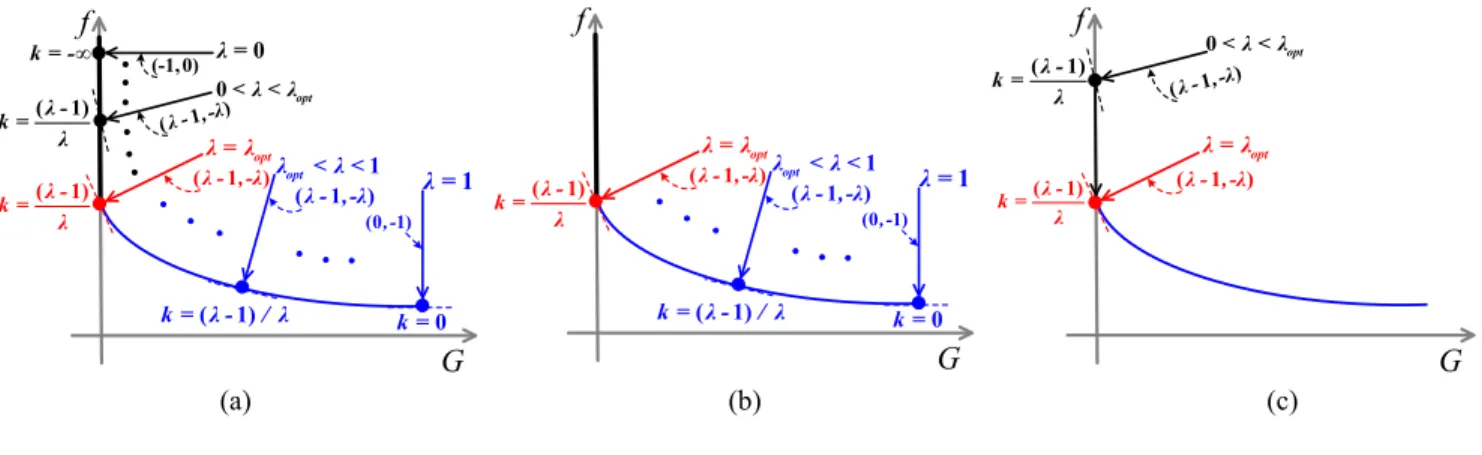
(a) (b) (c) Fig. 2. Weight vectors withλdistributed between 0 and 1. (a) 0≤λ≤1. (b)λopt< λ≤1. (c) 0< λ≤λopt.
Step 1.3: Generate a random population with NP indi-viduals: P = {x1, . . . ,xNP}, and evaluate P: FV =
{(f(x1),G(x1)), . . . , (f(xNP),G(xNP))}. Step 2 (Population Updating):
Step 2.1: Generate an offspring population OP =
{y1, . . . ,yNP}by executing the search algorithm. For i=1, . . . ,NP do
Step 2.2: Evaluateyi:(f(yi),G(yi)).
Step 2.3: For the index in Br(i) (i.e., i), if gws(yi|(λi,1−
λi)) ≤ gws(xi|(λi,1−λi)), set xi = yi, f(xi) = f(yi), and G(xi)=G(yi).
Step 3: Execute the weight vector adjusting strategy to adjust ηadaptively, and generate a set of NP weight vectors, i.e., {(λ1,1−λ1), . . . , (λNP,1−λNP)}, by utilizingη.
Step 4: Executing the restart strategy.
Step 5 (Stopping Criterion): If the stopping criterion is satisfied, then stop and output the feasible solution with the smallest objective function value; otherwise, go to step 2).
As the above description, DeCODE shares the same frame-work with decomposition-based multiobjective optimization except for steps 3 and 4. Step 3 is designed to make decomposition-based framework suit the properties of COPs. In addition, step 4 is developed to cope with extremely com-plicated constraints. Due to its numerous advantages, such as ease of implementation, powerful search ability, and few algorithm-specific parameters, DE is employed to design the search algorithm in this paper. It is worth noting that prior to calculating the weighted sum ofxi, its objective function value and degree of constraint violation are normalized as follows:
fnorm(xi)= f(xi)−fmin fmax−fmin (5) Gnorm(xi)= G(xi)−Gmin Gmax−Gmin (6)
where fminand fmaxare the minimum and maximum objective function values in P, respectively, and Gmin and Gmaxare the minimum and maximum degree of constraint violation in P, respectively.
Afterward, the weighted sum ofxi is calculated as follows: gwsxi(λi,1−λi) =λifnorm(xi)+(1−λi)Gnorm(xi) (7) where λi= i NP·η. (8)
Remark 1: Compared with conventional mathematical pro-gramming methods, the advantages of DeCODE are summa-rized as follows.
1) Since DeCODE is population-based, it is more robust. 2) DeCODE does not impose strong assumptions, such
as linearity, convexity, and differentiability on objective function and constraints, which makes it applicable to diverse kinds of COPs.
Remark 2: Compared with other COEAs, the advantages of DeCODE are twofold.
1) It shares the same framework with decomposition-based multiobjective optimization. Thus, the superiorities of the decomposition-based method (such as efficiency and collaborative evolution) can be inherited. Besides, the valuable knowledge developed for decomposition-based multiobjective optimization can be borrowed to further improve DeCODE.
2) The weighted sum method is easy to implement. Moreover, it provides an effective way for constrained optimization. The reason is explained in the follow-ing. The aim of constrained optimization is to locate the feasible optimum on the Pareto front (as shown in Fig. 1), rather than a set of Pareto optimal solu-tions uniformly distributed on the whole Pareto front. Hence, the transformed BOP can be regarded as a BOP with a discrete Pareto optimal solution. As analyzed in [13], the weighted sum method is more effective than the Tchebycheff decomposition approach on the multiobjective 0-1 knapsack problem, which also has discrete Pareto optimal solutions.
In the following sections, the weight vector adjusting strategy, the search algorithm, and the restart strategy are introduced sequentially.
B. Weight Vector Adjusting Strategy
The transformed BOP is optimized under the framework of decomposition-based multiobjective optimization. When a general BOP is solved, a set of representative solutions, the image of which is uniformly distributed on the whole Pareto
Fig. 3. Dynamic changing trajectory ofηwithα=0.5 and=30.
front, is desired. Hence, a set of uniformly distributed weight vectors across the whole objective space is always main-tained, where different weight vectors are expected to locate different points on the Pareto front. However, when the trans-formed BOP is solved, only the feasible optimum, which is the intersection of the f -axis and the Pareto front, is wanted. This difference indicates that a set of weight vectors for seeking the whole Pareto front is not suitable for locating the single feasible optimum. To address this issue, a weight vector adjust-ing strategy is designed to generate proper weight vectors for locating the feasible optimum.
In multiobjective optimization, it is well-known that a Pareto optimal solution of an MOP, under mild conditions, is the optimal solution of the weighted sum scalar optimization sub-problem with a weight vector(λ,1−λ)[13], [23]. Besides, as described in Fig.2(a), the slope of the tangent at the image of this Pareto optimal solution in the objective space is [(λ−1)/λ] and the corresponding direction vector is (λ−1,−λ) [23]. Furthermore, if the Pareto front is convex and differentiable, the slope of the tangent will increase monotonously with the increase of G [50]. That is to say, the bigger the value of G of a Pareto optimal solution, the bigger the value of the slope [(λ−1)/λ]. Because [(λ−1)/λ] increases monotonously with the increase ofλ, it is easy to know that the bigger the value of G, the bigger the value of λ, and vice versa.
Assuming that(λopt,1−λopt)is the weight vector attached to the feasible optimum, whose G is equal to 0, then the weight vector set {(λ,1−λ)|0 < λ ≤ 1} can be divided into two subsets as shown in Fig. 2(a), i.e., {(λ,1−λ)|0< λ≤λopt} and {(λ,1−λ)|λopt < λ ≤ 1}. The properties of these two subsets can be summarized as follows.
1) As shown in Fig. 2(b), the weight vector (λ,1 −λ) with λ ∈ (λopt,1] will locate a Pareto optimal solu-tion with G>0. That is to say, the weight vector with
λ∈(λopt,1] cannot achieve the feasible optimum. 2) As shown in Fig. 2(c), the weight vector (λ,1 −λ)
with λ ∈ (0, λopt] will seek a feasible solution first. Subsequently, guided by objective function (i.e., the f -axis), this feasible solution will approach the fea-sible optimum. To sum up, the weight vector with
λ∈(0, λopt] could achieve the feasible optimum finally. Based on the above analysis, a set of weight vectors
(λi,1−λi)(i ∈ {1, . . . ,NP}), where λi is generated between 0 andλopt, would be helpful to achieve the feasible optimum. However, it is not easy to generate such a set of weight vec-tors accurately due to the fact that λopt is problem-dependent
Algorithm 1: Weight Vector Adjusting Strategy
1 Set WV= ∅; 2 if flag==0 then 3 if Tt ≤pthen 4 ε=ε0(1−Tt)cp; 5 else 6 ε=0;
7 Calculate FeaPro of the population;
8 if FeaPro≥0.85 then 9 ε=0; 10 if Gmin≥εthen 11 flag=1; 12 η=10−18; 13 else 14 η= 1 1+e(t/T−α) ; 15 else 16 η=10−18; 17 for i=1 to NP do 18 λi=NPi ·η; 19 WV=WV∪(λi,1−λi);
and cannot be known beforehand. In this paper, a simple yet effective method is proposed to approximate this set of weight vectors by decreasing the parameter η dynamically accord-ing to the famous sigmoid function, which has been widely employed in the community of evolutionary computation [19]
η= 1
1+e(t/T−α) (9)
where t is the current generation number, T is the maximum generation number, and and α are two critical parameters to control the decreasing trend of η. As shown in Fig. 3, η decreases in accordance with the sigmoid curve as the gen-eration increases. At the early stage, η is very likely to be bigger thanλopt. In this case, the weight vectors can be divided into two sets: one includes weight vectors withλ∈(0, λopt], and the other contains weight vectors with λ ∈ (λopt,1]. As discussed above, the first set of weight vectors can steer the solutions approaching the feasible optimum. Although the sec-ond set of weight vectors is not able to locate the feasible optimum directly, it can introduce the information of objec-tive function, as shown in (7). Such information is beneficial to promote the exploration in the infeasible region [51]–[53]. At the later stage,ηwill be smaller thanλopt. In this case, all of the generated weight vectors can motivate their solutions to find the feasible optimum. In summary, during the evolution, decreasingη based on (9) is a suitable way to generate a set of weight vectors, which has the potential to find the feasible optimum gradually.
As shown in (9) and Fig.3,ηdecreases slowly at the early stage. Whenλoptof a COP is tiny,ηmay be larger than it for a relatively long period. Meanwhile, the number of weight vec-tors withλ∈(λopt, η] would be much more than the number of weight vectors with λ ∈ (0, λopt]. Consequently, accord-ing to (7), much information of objective function will be used. Under this condition, much effort would be devoted to exploring the region around the Pareto front while neglecting the feasible optimum. To remedy this weakness, ηshould be truncated to a small value to suit λopt. As stated previously, we cannot know the value of λopt a priori, which signifies
that we cannot know whether ηneeds to be truncated or not. Hence, a proper indicator should be used to reflect whether decreasing η according to (9) is suitable for the considered COP. Intuitively, if the decreasing manner ofηis suitable for a COP, the degree of constraint violation would decrease consis-tently. Thus, we try to set a target level of degree of constraint violation at each generation. Once the target level cannot be satisfied, we consider that decreasingηaccording to (9) is not suitable. Under this condition, η is truncated to an extremely small value to guarantee that the number of weight vectors with λ ∈ (0, λopt] is as many as possible. By this way, the feasible optimum could be achieved.
To set the target level at each generation, based on [51], the
ε level controlling method is utilized here
ε= ε0 1−Ttcp, if Tt ≤p 0, otherwise (10) cp= −logε0+β log(1−p) (11)
where ε0 is the initial level, β is set to 6 in this paper, and
p is an important parameter to control the target level at each generation. Similar to [51], in order to improve the usability, if the feasible proportion, i.e., FeaPro, exceeds FP (i.e., 0.85),
ε is set to 0. As shown in (10),ε decreases with the increase of generation.
The whole process of the weight vector adjusting strategy is described in Algorithm 1. As shown in Algorithm 1, ε is the target level at each generation and Gmin ≥ ε means that the target level cannot be fulfilled. Besides, η is truncated to an extremely small valueηL (i.e., 10−18) rather than 0. In this case, the information of objective function can be utilized to some extent.
C. Search Algorithm
When a search algorithm is designed for constrained optimization, it is expected to make a tradeoff not only between convergence and diversity, but also between con-straints and objective function. In this paper, two DE trial vector generation strategies are integrated to achieve this goal, which are described below [54], [55].
1) DE/rand-to-best/1/bin vi= xr1+F· xbest− xr1 +F·xr2− xr3 (12) ui,j= vi,j, if randj<CR or j=jrand xi,j, otherwise. ,j=1, . . . ,D (13) 2) DE/current-to-rand/1 ui= xi+rand· xr1− xi +F·xr2 − xr3 (14) where xi, vi, and ui are the ith target vector, the ith mutant vector, and the ith trial vector, respectively, xi,j, vi,j, and ui,j are the jth dimension of them, respectively,
xr1, xr2, and xr3 are three mutually different
individu-als randomly selected from the population, xbest is the individual with the best performance, F is the scaling factor, CR is the crossover control parameter, and jrand is a random integer chosen from{1, . . . ,D}.
Algorithm 2: Search Algorithm
1 Set OP= ∅;
2 for i=1 to NP do
3 Calculate fnorm(xi)and Gnorm(xi)according to (5) and (6), respectively;
4 for i=1 to NP do
5 Randomly select a F value from the pool{0.6,0.8,1.0};
6 Randomly select a CR value from the pool{0.1,0.2,1.0};
7 if rand<Tt then
8 Set WSi= ∅;
9 for j=1 to NP do
10 WSi=WSi∪gws(xj|(λi,1−λi));
11 Selectxbestbased on WSi;
12 Selectxr1,xr2, andxr3from the population;
13 Generate an offspringuiaccording to (12) and (13);
14 else
15 Selectxr1,xr2, andxr3from the population;
16 Generate an offspringuiaccording to (14);
17 OP=OP∪ ui;
With respect to (12), the information of the best individ-ual is utilized to generate a mutant vector. Consequently, the convergence can be accelerated via this strategy. Besides, in terms of (14), xi learns the information of a randomly selected individual xr1. Therefore, this strategy can promote
the diversity.
These two strategies are combined in the following man-ner. For each individual, DE/rand-to-best/1/bin is executed with the probability (t/T)while DE/current-to-rand/1 is con-ducted with the probability [1−(t/T)], where t and T are the current and maximum generation number, respectively. At the early stage, (t/T) is small. So DE/current-to-rand/1 will be used more frequently for exploration. At the later stage,
(t/T)becomes large. Thus, DE/rand-to-best/1/bin will be uti-lized more often for exploitation. By this manner, the tradeoff between convergence and diversity can be achieved.
How to select the best individual in (12) has a direct effect on the tradeoff between constraints and objective function. In general, to achieve such a tradeoff, much information of objec-tive function should be preferred at the early stage while little information of objective function should be favorable at the later stage. It is because much information of objective func-tion is beneficial to promote the explorafunc-tion in the infeasible region [51]–[53], while little information of objective func-tion can promote the convergence to the feasible optimum. In this paper, the best individual is selected according to the weighted sum. First, the normalized objective function value and degree of constraint violation are calculated for each indi-vidual according to (5) and (6), respectively. Afterward, a set of weighted sum is obtained on the basis ofλi
WSi=
gws(x1|(λi,1−λi)), . . . ,gws(xNP|(λi,1−λi)) . (15) Finally, the individual with the minimum value in WSi is selected as the best individual forxi. By doing this, each indi-vidual xi can evolve along its own direction defined by the weight vector(λi,1−λi). By making use of the weight vector adjusting strategy illustrated in SectionIV-B, the information of objective function can be utilized properly and a tradeoff between constraints and objective function can be achieved.
TABLE I
MAXIMUMNUMBER OFFUNCTIONEVALUATIONS
MaxFEsANDPOPULATIONSIZENP
Therefore, the above process is able to strike a tradeoff not only between convergence and diversity but also between constraints and objective function. In addition, two control parameters in DE, i.e., F and CR, are set in the same way as in [54]. The details of the search algorithm are summarized in Algorithm 2.
D. Restart Strategy
In practice, some COPs may involve complicated con-straints with strong nonlinearity and multimodality. Due to the complex infeasible region formed by these constraints, the population is very easy to stagnate. To address this issue, a restart strategy is introduced [55].
Before applying the restart strategy, one needs to answer a fundamental question: how to judge whether the popula-tion has already stagnated in the infeasible region or not. Intuitively, if the population converges to a small region in the infeasible region, the difference among the individuals will be tiny. Consequently, the individuals will have the similar degree of constraint violation or objective function values. Thus, we can conclude that the population has stagnated in the infeasible region when the following two conditions are satisfied.
1) All the individuals are infeasible.
2) All the individuals have the similar degree of con-straint violation or objective function values, i.e., the standard deviation of the degree of constraint violation or objective function values is less than a predefined thresholdμ.
Once these two conditions have been detected, the restart strategy will be triggered—all the solutions in the population will be regenerated from the decision space randomly. The reasons for regenerating the population randomly are twofold. First, if the population has stagnated in the infeasible region, the information contained by the population is not useful for searching for the optimal solution. Second, a possible way to avoid stagnation is to exploit the feedback information from the evolution to guide the optimization. However, under this condition, more storage space is required. More importantly, it is not easy to decide what feedback information is promising. Apparently, the thresholdμis critical to the restart strategy. A too big μmay lead to a wrong decision on the stagnation, which has a negative impact on convergence. On the contrary, a too small value cannot detect the stagnation timely, which would waste computational resources to some extent. Thus, it should be set carefully. We have investigated the setting of μ in the empirical study.
V. EMPIRICALSTUDY
A. Benchmark Test Functions and Parameter Settings Three sets of benchmark test functions were employed to demonstrate the performance of DeCODE. The first set includes 24 test functions from IEEE CEC2006 [56], the sec-ond set contains 18 test functions with ten-dimensions (10D) and 30-dimensions (30D) from IEEE CEC2010 [57], and the third set involves 28 test functions with 50-dimensions (50D), and 100-dimensions (100D) from IEEE CEC2017 [58]. Note that these three sets of test functions exhibit various difficult properties, such as strong nonlinearity, tiny feasible region, and rotated landscape. Thus, they are able to provide a sys-tematic assessment on the performance of DeCODE. More details about these three sets of test functions are referred to [56]–[58].
The maximum number of functions evaluations MaxFEs and the population size NP are described in TableI. Note that NP is varied with different test sets and is related to the dimension of the search space. Following the suggestions in [56]–[58], 25 independent runs were performed for each test function. In addition, the tolerance valueδ for equality constraints was set to 10−4. For DeCODE,ε0 was set to min(εL, Gmax0), where Gmax0is the maximum degree of constraint violation in the ini-tial population andεL=10D/2is used to avoid a too largeε0.
Moreover, in the sigmoid function,α in the sigmoid func-tion, p in theε level controlling method, andμ in the restart strategy were set to 30, 0.75, 0.85, and 10−6, respectively.
B. Experiments on the 24 Benchmark Test Functions From IEEE CEC2006
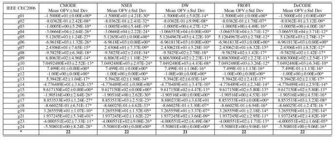
First, DeCODE was evaluated on the 24 benchmark test functions from IEEE CEC2006. Its performance was compared with four state-of-the-art COEAs with various constraint-handling techniques: CMODE [7], NSES [9], DW [48], and FROFI [54]. Note that CMODE and NSES are methods based on Pareto dominance. It can be known from [56] that it is extremely difficult to locate the optimum of g22 and there are no feasible solutions for g20. Thus, these two test functions were not considered here. The experimental results over 25 independent runs are summarized in Table II, where “Mean OFV” and “Std Dev” denote the average and standard devi-ation of objective function values over 25 runs, respectively. Due to the fact that the true optimum of each test function has been provided in [56], we can define a successful run as follows. A run for a test function is successful, if and only if f(xbest)−f(x∗) <10−4, wherex∗ is the optimum provided in [56] and xbest is the best feasible solution provided by a method. In TableII, “*” denotes that a method can satisfy the successful condition over all 25 runs for a test function.
It can be seen from Table IIthat among the five compared methods, CMODE, NSES, FROFI, and DeCODE can success-fully obtain the optima of all test functions. However, DW cannot find the optimum of g17 consistently. In summary, the experimental results validate that DeCODE yields better or similar performance compared with other four competitors on the 24 test functions from IEEE CEC2006.
TABLE II
EXPERIMENTALRESULTS OFDECODEANDFOUROTHERSELECTEDMETHODSOVER 25 INDEPENDENTRUNS ON22 TESTFUNCTIONSFROMIEEE CEC2006
TABLE III
EXPERIMENTALRESULTS OFDECODEANDFIVEOTHERSELECTEDMETHODSOVER 25 INDEPENDENTRUNS ON18 TESTFUNCTIONSWITH10D FROMIEEE CEC2010
TABLE IV
RESULTS OF THEMULTIPLE-PROBLEMWILCOXON’STEST FORDECODE ANDFIVEOTHERSELECTEDMETHODS ON18 TESTFUNCTIONS
WITH10D FROMIEEE CEC2010
C. Experiments on the 18 Benchmark Test Functions With 10D and 30D From IEEE CEC2010
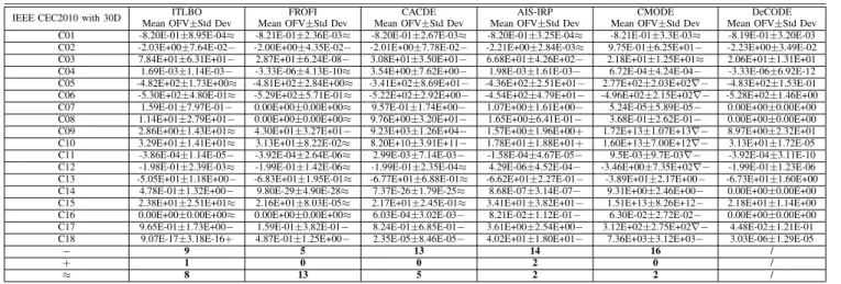
Subsequently, 36 complicated test functions from IEEE CEC2010 were taken into account. Due to the fact that the optimal solutions of these test functions are unknown, the aver-age and standard deviation of objective function values over 25 runs were taken as the comparison criteria. Five state-of-the-art methods with various constraint-handling techniques
TABLE V
RANKING OFDECODEANDFIVEOTHERSELECTEDMETHODS BY THEFRIEDMAN’STEST ON18 TESTFUNCTIONS
WITH10D FROMIEEE CEC2010
were selected as the competitors: ITLBO [59], FROFI [54], CACDE [60], AIS-IRP [61], and DW [48]. The experimen-tal results of ITLBO and FROFI can be available from our previous study. So the Wilcoxon’s rank sum test at a 0.05 significance level was used to compare DeCODE with each of ITLBO and FROFI. We can just obtain the average and standard deviation of objective function values of CACDE,
TABLE VI
EXPERIMENTALRESULTS OFDECODEANDFIVEOTHERSELECTEDMETHODSOVER 25 INDEPENDENTRUNS ON18 TESTFUNCTIONSWITH30D FROMIEEE CEC2010
TABLE VII
RESULTS OF THEMULTIPLE-PROBLEMWILCOXON’STEST FORDECODE ANDFIVEOTHERSELECTEDMETHODS ON18 TESTFUNCTIONS
WITH30D FROMIEEE CEC2010
AIS-IRP, and DW from their original papers. Thus, the t-test at a 0.05 significance level was adopted to compare each of them with DeCODE. Furthermore, to compare these six methods simultaneously, the multiple-problem Wilcoxon’s test and the Friedman’s test were implemented via KEEL software [62]. Note that the Bonferroni–Dunn method was selected as the post-hoc method of the Friedman’s test.
Regarding the test functions with 10D, the average and stan-dard deviation of objective function values over 25 runs, results of the multiple-problem Wilcoxon’s test, and results of the Friedman’s test are summarized in Tables III–V, respectively. In Table III, “∇” denotes that feasible solutions cannot be found by a method consistently over 25 runs, and “−”, “+”, and “≈” represent that the performance of the correspond-ing competitor is worse than, better than, and similar to that of DeCODE in terms of the Wilcoxon’s rank sum test/t-test, respectively. As shown in Table III, DeCODE performs bet-ter than ITLBO, FROFI, CACDE, AIS-IRP, and DW on five, six, five, 12, and eight test functions, respectively. In contrast, these five competitors outperform DeCODE on four, two, four, six, and six test functions, respectively. Note that DW can-not find any feasible solution on C11 and the experimental results of C11 are not provided in its original literature. In Table IV, all the R+ values are bigger than the R− values, which reflects that the performance of DeCODE is superior to that of five other competitors. Moreover, DeCODE achieves the first rank in the Friedman’s test. Therefore, the experi-mental results demonstrate that DeCODE outperforms the five
TABLE VIII
RANKING OFDECODEANDFIVEOTHERSELECTEDMETHODS BY THEFRIEDMAN’STEST ON18 TESTFUNCTIONS
WITH30D FROMIEEE CEC2010
other competitors on the 18 test functions with 10D from IEEE CEC2010.
In terms of the test functions with 30D, the average and standard deviation of objective function values over 25 runs, results of the multiple-problem Wilcoxon’s test, and results of the Friedman’s test are reported in TablesVI–VIII, respec-tively. Note that, since the experimental results of DW on 30D cannot be obtained from the original paper [48], we removed DW and added CMODE [7] as a compared method. As shown
in TableVI, DeCODE outperforms ITLBO, FROFI, CACDE,
AIS-IRP, and CMODE on nine, five, 13, 14, and 16 test functions, respectively. However, ITLBO, FROFI, CACDE, AIS-IRP, and CMODE cannot surpass DeCODE on more than two test functions. In Table VII, all the R+ values are big-ger than the R−values, which reflects that the performance of DeCODE is better than that of the five competitors. Moreover, the significant difference at α = 0.1 can be observed in all cases and the significant difference atα=0.05 can be found in four cases, i.e., DeCODE versus ITLBO, DeCODE ver-sus CACDE, DeCODE verver-sus AIS-IRP, and DeCODE verver-sus CMODE. From TableVIII, DeCODE ranks the first according to the Friedman’s test. Considering the experimental results, we can conclude that DeCODE has an edge over the five competitors on the 18 test functions with 30D from IEEE CEC2010.
To test the computational efficiency of DeCODE, its com-putational time was compared with CMODE, whose source
code can be obtained online, on the 36 test functions from IEEE CEC2010. Note that CMODE is a Pareto dominance-based method. The experiments were performed on a computer with Intel Core i7-3770 (3.40 GHz) processor and Windows10 (64 bit) system. These two algorithms were programmed in MATLAB. The computational time provided by DeCODE is 139.55 s and 429.55 s for the 18 test functions with 10D and 30D over one run, respectively. The corresponding computa-tional time resulting from CMODE is 200.84 s and 653.44 s, respectively. Thus, DeCODE is more efficient than CMODE, which also verifies that the decomposition-based framework is more efficient than nondominated sorting [13], [19].
In view of all the above experimental results, DeCODE shows overall better performance than the five competitors.
D. Experiments on the 28 Benchmark Test Functions With 50D and 100D From IEEE CEC2017
The 28 test functions with 50D and 100D from IEEE CEC2017 [58] were adopted to further evaluate DeCODE’s performance on high-dimensional COPs. The two best algo-rithms, i.e., LSHADE44 [63] and UDE [64], in the IEEE CEC2017 competition were selected as the competitors. We compared DeCODE with each of LSHADE44 and UDE according to the ranking procedure provided in IEEE CEC2017.
1) Rank the methods based on the feasible rate (FR), which denotes the percentage of runs where at least one feasible solution is found.
2) Then rank the methods according to the average degree of constraint violation (voi).
3) Finally, rank the methods in terms of the average objective function value.
To compare these three algorithms concurrently, we first ranked them on each test function according to the above procedure. Afterward, the total rank on all test functions was calculated. The experimental results are summarized in Table S-1 in the supplementary material. As shown in Table S-1, the total ranks of DeCODE on the 28 test functions with 50D and 100D are 45 and 44, respectively. Compared with DeCODE, the corresponding total ranks achieved by both LSHADE44 and UDE are larger. Therefore, DeCODE is bet-ter than LSHADE44 and UDE on these 56 test functions, which means that DeCODE has good scalability in solving high-dimensional COPs.
E. Effectiveness of the Weight Vector Adjusting Strategy As introduced in Section IV-B, the weight vector adjusting strategy is used to generate proper weight vectors for locating the feasible optimum of a COP. To investigate the effectiveness of this strategy, five variants of DeCODE were implemented by setting ηto five fixed values, i.e., η=0.1, η=0.3, η= 0.5, η = 0.7, and η = 1.0. The performance of DeCODE and these five variants was evaluated on the 18 test functions with 30D from IEEE CEC2010. Similar to Section V-C, the average and standard deviation of objective function values were recorded. In addition, if an algorithm fails to find at least
one feasible solution consistently over 25 runs, the feasible rate was provided.
The Wilcoxon’s rank sum test at a 0.05 significance level was used for performance comparison. The experimental results are summarized in Table S-2 in the supplementary material. As shown in Table S-2, DeCODE performs better than its five variants on 13, 14, 10, seven, and five test func-tions, respectively. However, these five variants cannot surpass DeCODE on more than one test function. The experimental results validate that the weight vector adjusting strategy plays a key role in making the decomposition-based framework suit the properties of COPs.
F. Effectiveness of the Search Algorithm
We implemented six variants of DeCODE, where six different search algorithms were adopted. To be specific, in DeCODE-ConCon, the best individual in DE/rand-to-best/1/bin was selected based on G(x). In DeCODE-ConObj, the best individual in DE/rand-to-best/1/bin was selected according to f(x). In DeCODE-Con and DeCODE-Obj, only DE/rand-to-best/1/bin was used. Note that the best indi-vidual was selected based on G(x) in DeCODE-Con and based on f(x)in DeCODE-Obj, respectively. In DeCODE-Div, DE/current-to-rand/1 was employed as the search algorithm while DE/rand/1/bin was used as the search algorithm in DeCODE-rand1. These six variants were evaluated on the 18 test functions with 30D from IEEE CEC2010. The experi-mental results are collected in Table S-3 in the supplementary material. Note that the performance of these six variants was compared with that of DeCODE based on the Wilcoxon’s rank sum test at a 0.05 significance level.
From Table S-3, DeCODE outperforms the six variants on six, two, 14, eight, 18, and 16 test functions, respectively. However, no variant can provide better results on more than two test functions than DeCODE. By comparing DeCODE with DeCODE-ConCon and DeCODE-ConObj, it can be seen that properly utilizing f(x)/G(x) is critical to a search algo-rithm. That is to say, the tradeoff between constraints and objective function is critical. By comparing DeCODE with Con, Obj, Div, and DeCODE-rand1, we can find that the tradeoff between diversity and convergence is also important for a search algorithm. In sum-mary, the effectiveness of the proposed search algorithm has been confirmed.
G. Effectiveness of the Sigmoid Function
As described in Section IV-B, the sigmoid function con-trols the decreasing trend of η. As we know, the linear function and the exponential function are two other popular functions that can be used to control a dynamic parame-ter. To this end, we implemented two variants of DeCODE, i.e., DeCODE-Lin and DeCODE-Exp, which made use of the linear function [i.e.,η=1−(t/T)] and the exponential func-tion (i.e., η = [e30(1−t/T)−1]/(e30−1)), respectively. The performance of DeCODE, DeCODE-Lin, and DeCODE-Exp was evaluated on the 36 test functions from IEEE CEC2010.
TABLE IX
EXPERIMENTALRESULTS OFDECODEANDDECODE-WOR OVER25 INDEPENDENTRUNS ONTHREETESTFUNCTIONS
The experimental results are summarized in Table S-4 in the supplementary material.
As shown in Table S-4, compared with DeCODE-Exp, DeCODE shows better performance on more test functions in terms of both 10D and 30D. Although DeCODE-Lin performs better than DeCODE on the 18 test functions with 10D, it is worse than DeCODE on the 18 test func-tions with 30D. Moreover, DeCODE-Lin cannot consistently find feasible solutions on C05 with 30D. Therefore, the experimental results verify the advantage of the sigmoid function.
H. Effectiveness of the Weighted Sum Method
We compared DeCODE with another variant, i.e.,
DeCODE-Tch, where the weighted sum method was replaced with the Tchebycheff decomposition approach. Both DeCODE and DeCODE-Tch were evaluated on the 36 test func-tions from IEEE CEC2010 and the experimental results are summarized in Table S-5 in the supplementary mate-rial. As shown in Table S-5, DeCODE-Tch cannot beat DeCODE on any test function while DeCODE provides bet-ter results on ten test functions. The experimental results reflect the superiority of the weighted sum method for con-strained optimization, which is in line with the analysis in SectionIV-A.
I. Effectiveness of the Restart Strategy
In order to validate the effectiveness of the restart strategy, a competitor called DeCODE-WoR was implemented by remov-ing the restart strategy from DeCODE. The 36 test functions from IEEE CEC2010 were used to produce the experimental results.
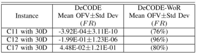
Similar to Section V-E, the average and standard devia-tion of objective funcdevia-tion values and the feasible rate were recorded. Significant difference can be observed on three test functions, i.e., C11 with 30D, C12 with 30D, and C17 with 30D, based on the Wilcoxon’s rank sum test at a 0.05 sig-nificance level. The experimental results of these three test functions are summarized in Table IX.
As shown in Table IX, on C11 with 30D, C12 with 30D, and C17 with 30D, DeCODE-WoR tends to be trapped in the infeasible region. Specifically, DeCODE-WoR converges to a local optimum in the infeasible region on these three test functions over six, one, and five runs, respectively.
In summary, the restart strategy can help the population jump out of the infeasible area where it has stagnated.
Remark 3: In Section S-I in the supplementary material, we also analyzed the effect of the parameter settings on the performance of DeCODE by extensive experiments.
VI. CONCLUSION
This paper further developed the potential of decomposition-based multiobjective optimization for constrained evolutionary optimization. In this paper, a COP was first transformed into a BOP. Thereafter, the transformed BOP was opti-mized under the decomposition-based framework. In order to make decomposition-based multiobjective optimization suit the properties of COPs, a weight vector adjusting strategy was proposed. In addition, DE was used to design the search algo-rithm. Moreover, a restart strategy was introduced to tackle COPs with complicated constraints. By the above process, an alternative COEA, i.e., DeCODE, was presented. Extensive and systematic experiments verified that the following.
1) The weight vector adjusting strategy is an effec-tive way to adapt decomposition-based multiobjeceffec-tive optimization for COPs, by producing appropriate weight vectors.
2) The restart strategy improves DeCODE’s ability to find feasible solutions for COPs with complicated constraints.
3) DeCODE shows superior performance against some state-of-the-art COEAs including Pareto dominance-based methods on three sets of benchmark test functions. In the future, it is interesting to extend DeCODE to solve constrained MOPs. Note that, as an EA, the optimality and convergence of DeCODE cannot be theoretically guaranteed as conventional mathematical programming methods, especially in the scenarios which have high requirements for real-time performance and optimality [65], [66]. In the future, we will try to investigate COEAs from theoretical aspects.
The MATLAB source code of DeCODE can be down-loaded from Y. Wang’s homepage: http://www.escience.cn/ people/yongwang1/index.html.
REFERENCES
[1] Y.-H. Jia et al., “A dynamic logistic dispatching system with set-based particle swarm optimization,” IEEE Trans. Syst., Man, Cybern., Syst., vol. 48, no. 9, pp. 1607–1621, Sep. 2018.
[2] L. Ma et al., “Two-level master–slave RFID networks planning via hybrid multiobjective artificial bee colony optimizer,” IEEE Trans. Syst.,
Man, Cybern., Syst., to be published, doi:10.1109/TSMC.2017.2723483. [3] T. Ray, T. Kang, and S. K. Chye, “An evolutionary algorithm for con-strained optimization,” in Proc. 2nd Annu. Conf. Genet. Evol. Comput., 2000, pp. 771–777.
[4] A. H. Aguirre, S. B. Rionda, C. A. Coello Coello, G. L. Lizárraga, and E. M. Montes, “Handling constraints using multiobjective optimization concepts,” Int. J. Numer. Methods Eng., vol. 59, no. 15, pp. 1989–2017, 2004.
[5] Z. Cai and Y. Wang, “A multiobjective optimization-based evolutionary algorithm for constrained optimization,” IEEE Trans. Evol. Comput., vol. 10, no. 6, pp. 658–675, Dec. 2006.
[6] Y. Wang, Z. Cai, G. Guo, and Y. Zhou, “Multiobjective optimization and hybrid evolutionary algorithm to solve constrained optimization prob-lems,” IEEE Trans. Syst., Man, Cybern. B, Cybern., vol. 37, no. 3, pp. 560–575, Jun. 2007.
[7] Y. Wang and Z. Cai, “Combining multiobjective optimization with dif-ferential evolution to solve constrained optimization problems,” IEEE
[8] Y. Wang and Z. Cai, “A dynamic hybrid framework for constrained evolutionary optimization,” IEEE Trans. Syst., Man, Cybern. B, Cybern., vol. 42, no. 1, pp. 203–217, Feb. 2012.
[9] L. Jiao, L. Li, R. Shang, F. Liu, and R. Stolkin, “A novel selection evolutionary strategy for constrained optimization,” Inf. Sci., vol. 239, pp. 122–141, Aug. 2013.
[10] N. Dong and Y. Wang, “An unbiased bi-objective optimization model and algorithm for constrained optimization,” Int. J. Pattern Recognit.
Artif. Intell., vol. 28, no. 8, 2014, Art. no. 1459008.
[11] T. Xu, J. He, C. Shang, and W. Ying, “A new multi-objective model for constrained optimisation,” in Advances in Computational Intelligence
Systems. Cham, Switzerland: Springer, 2017, pp. 71–85.
[12] P. C. Roy, K. Deb, and M. M. Islam, “An efficient nondominated sort-ing algorithm for large number of fronts,” IEEE Trans. Cybern., to be published, doi:10.1109/TCYB.2017.2789158.
[13] Q. Zhang and H. Li, “MOEA/D: A multiobjective evolutionary algorithm based on decomposition,” IEEE Trans. Evol. Comput., vol. 11, no. 6, pp. 712–731, Dec. 2007.
[14] A. Trivedi, D. Srinivasan, K. Sanyal, and A. Ghosh, “A survey of multiobjective evolutionary algorithms based on decomposition,” IEEE
Trans. Evol. Comput., vol. 21, no. 3, pp. 440–462, Jun. 2017.
[15] M. Elarbi, S. Bechikh, A. Gupta, L. B. Said, and Y.-S. Ong, “A new decomposition-based NSGA-II for many-objective optimization,”
IEEE Trans. Syst., Man, Cybern., Syst., vol. 48, no. 7, pp. 1191–1210,
Jul. 2018.
[16] Q. Zhang, W. Liu, and H. Li, “The performance of a new version of MOEA/D on CEC09 unconstrained MOP test instances,” in Proc. IEEE
Congr. Evol. Comput., 2009, pp. 203–208.
[17] Q. Kang, X. Song, M. Zhou, and L. Li, “A collaborative resource allocation strategy for decomposition-based multiobjective evolutionary algorithms,” IEEE Trans. Syst., Man, Cybern., Syst., to be published, doi:10.1109/TSMC.2018.2818175.
[18] H. Ishibuchi, Y. Sakane, N. Tsukamoto, and Y. Nojima, “Evolutionary many-objective optimization by NSGA-II and MOEA/D with large populations,” in Proc. IEEE Int. Conf. Syst. Man Cybern., 2009, pp. 1758–1763.
[19] Z. Wang, Q. Zhang, A. Zhou, M. Gong, and L. Jiao, “Adaptive replace-ment strategies for MOEA/D,” IEEE Trans. Cybern., vol. 46, no. 2, pp. 474–486, Feb. 2016.
[20] T. P. Runarsson and X. Yao, “Search biases in constrained evolutionary optimization,” IEEE Trans. Syst., Man, Cybern. C, Appl. Rev., vol. 35, no. 2, pp. 233–243, May 2005.
[21] X. Li and G. Zhang, “Biased multiobjective optimization for constrained single-objective evolutionary optimization,” in Proc. 11th IEEE World
Congr. Intell. Control Autom. (WCICA), 2014, pp. 891–896.
[22] L. Wang, Q. Zhang, A. Zhou, M. Gong, and L. Jiao, “Constrained subproblems in a decomposition-based multiobjective evolutionary algo-rithm,” IEEE Trans. Evol. Comput., vol. 20, no. 3, pp. 475–480, Jun. 2016.
[23] K. Miettinen, Nonlinear Multiobjective Optimization, vol. 12. New York, NY, USA: Springer, 2012.
[24] C. A. Coello Coello, “Treating constraints as objectives for single-objective evolutionary optimization,” Eng. Optim., vol. 32, no. 3, pp. 275–308, 2000.
[25] C. A. Coello Coello and E. M. Montes, “Constraint-handling in genetic algorithms through the use of dominance-based tournament selection,”
Adv. Eng. Informat., vol. 16, no. 3, pp. 193–203, 2002.
[26] J. D. Schaffer, “Multiple objective optimization with vector evaluated genetic algorithms,” in Proc. 1st Int. Conf. Genet. Algorithms Appl., 1985, pp. 93–100.
[27] J. Horn, N. Nafpliotis, and D. E. Goldberg, “A niched Pareto genetic algorithm for multiobjective optimization,” in Proc. 1st IEEE Conf. Evol.
Comput., 1994, pp. 82–87.
[28] T. Ray and K. M. Liew, “Society and civilization: An optimization algo-rithm based on the simulation of social behavior,” IEEE Trans. Evol.
Comput., vol. 7, no. 4, pp. 386–396, Aug. 2003.
[29] A. Angantyr, J. Andersson, and J.-O. Aidanpaa, “Constrained optimization based on a multiobjective evolutionary algorithm,” in Proc.
IEEE Congr. Evol. Comput., vol. 3, 2003, pp. 1560–1567.
[30] J. Knowles and D. Corne, “The Pareto archived evolution strategy: A new baseline algorithm for Pareto multiobjective optimisation,” in Proc.
IEEE Congr. Evol. Comput., vol. 1, 1999, pp. 98–105.
[31] Y. Zhou, Y. Li, J. He, and L. Kang, “Multi-objective and MGG evolu-tionary algorithm for constrained optimization,” in Proc. IEEE Congr.
Evol. Comput., vol. 1, 2003, pp. 1–5.
[32] Y. Wang, Z. Cai, Y. Zhou, and W. Zeng, “An adaptive tradeoff model for constrained evolutionary optimization,” IEEE Trans. Evol. Comput., vol. 12, no. 1, pp. 80–92, Feb. 2008.
[33] Y. Wang and Z. Cai, “Constrained evolutionary optimization by means of (μ+λ)-differential evolution and improved adaptive trade-off model,”
Evol. Comput., vol. 19, no. 2, pp. 249–285, 2011.
[34] G. Jia, Y. Wang, Z. Cai, and Y. Jin, “An improved (μ+λ)-constrained differential evolution for constrained optimization,” Inf. Sci., vol. 222, pp. 302–322, Feb. 2013.
[35] G. Venter and R. Haftka, “Constrained particle swarm optimization using a bi-objective formulation,” Struct. Multidiscipl. Optim., vol. 40, nos. 1–6, p. 65, 2010.
[36] W. Gong, Z. Cai, and D. Liang, “Engineering optimization by means of an improved constrained differential evolution,” Comput. Methods Appl.
Mech. Eng., vol. 268, pp. 884–904, Jan. 2014.
[37] S. Venkatraman and G. G. Yen, “A generic framework for constrained optimization using genetic algorithms,” IEEE Trans. Evol. Comput., vol. 9, no. 4, pp. 424–435, Aug. 2005.
[38] K. Deb, A. Pratap, S. Agarwal, and T. Meyarivan, “A fast and elitist multiobjective genetic algorithm: NSGA-II,” IEEE Trans. Evol. Comput., vol. 6, no. 2, pp. 182–197, Apr. 2002.
[39] K. Masuda and K. Kurihara, “A constrained global optimization method based on multi-objective particle swarm optimization,” Electron.
Commun. Japan, vol. 95, no. 1, pp. 43–54, 2012.
[40] K. Deb and R. Datta, “A bi-objective constrained optimization algorithm using a hybrid evolutionary and penalty function approach,” Eng. Optim., vol. 45, no. 5, pp. 503–527, 2013.
[41] R. Datta and K. Deb, “Individual penalty based constraint handling using a hybrid bi-objective and penalty function approach,” in Proc. IEEE
Congr. Evol. Comput. (CEC), 2013, pp. 2720–2727.
[42] R. Datta and K. Deb, “Uniform adaptive scaling of equality and inequal-ity constraints within hybrid evolutionary-cum-classical optimization,”
Soft Comput., vol. 20, no. 6, pp. 2367–2382, 2016.
[43] R. Datta, K. Deb, and A. Segev, “A bi-objective hybrid constrained optimization (HyCon) method using a multi-objective and penalty func-tion approach,” in Proc. IEEE Congr. Evol. Comput. (CEC), 2017, pp. 317–324.
[44] S. Watanabe and K. Sakakibara, “Multi-objective approaches in a single-objective optimization environment,” in Proc. IEEE Congr. Evol.
Comput., vol. 2, 2005, pp. 1714–1721.
[45] L. Gao, Y. Zhou, X. Li, Q. Pan, and W. Yi, “Multi-objective optimization based reverse strategy with differential evolution algorithm for con-strained optimization problems,” Expert Syst. Appl., vol. 42, no. 14, pp. 5976–5987, 2015.
[46] X. Li, S. Zeng, C. Li, and J. Ma, “Many-objective optimization with dynamic constraint handling for constrained optimization problems,”
Soft Comput., vol. 21, no. 24, pp. 7435–7445, 2017.
[47] S. Zeng, R. Jiao, C. Li, X. Li, and J. S. Alkasassbeh, “A general framework of dynamic constrained multiobjective evolutionary algo-rithms for constrained optimization,” IEEE Trans. Cybern., vol. 47, no. 9, pp. 2678–2688, Sep. 2017.
[48] C. Peng, H.-L. Liu, and F. Gu, “A novel constraint-handling technique based on dynamic weights for constrained optimization problems,” Soft
Comput., vol. 22, no. 12, pp. 3919–3935, 2018.
[49] K. Deb, “An efficient constraint handling method for genetic algorithms,”
Comput. Methods Appl. Mech. Eng., vol. 186, no. 2, pp. 311–338, 2000.
[50] S. Boyd and L. Vandenberghe, Convex Optimization. Cambridge, U.K.: Cambridge Univ. Press, 2004.
[51] T. Takahama and S. Sakai, “Efficient constrained optimization by theε constrained adaptive differential evolution,” in Proc. IEEE Congr. Evol.
Comput., 2010, pp. 1–8.
[52] T. Takahama and S. Sakai, “Efficient constrained optimization by the
ε constrained rank-based differential evolution,” in Proc. IEEE Congr.
Evol. Comput., 2012, pp. 1–8.
[53] J. Liu, K. L. Teo, X. Wang, and C. Wu, “An exact penalty function-based differential search algorithm for constrained global optimization,”
Soft Comput., vol. 20, no. 4, pp. 1305–1313, 2016.
[54] Y. Wang, B.-C. Wang, H.-X. Li, and G. G. Yen, “Incorporating objective function information into the feasibility rule for constrained evolutionary optimization,” IEEE Trans. Cybern., vol. 46, no. 12, pp. 2938–2952, Dec. 2016.
[55] B.-C. Wang, H.-X. Li, J.-P. Li, and Y. Wang, “Composite differential evolution for constrained evolutionary optimization,” IEEE Trans. Syst.,
Man, Cybern., Syst., to be published, doi:10.1109/TSMC.2018.2807785. [56] J. J. Liang et al., “Problem definitions and evaluation criteria for the CEC 2006 special session on constrained real-parameter optimization,”