Lift-based search for significant dependencies in dense data sets

(1)

Lift-based search for significant dependencies in dense

data sets

W. Hämäläinen

Department of Computer Science

University of Helsinki Finland

[email protected]

ABSTRACT

Dependency analysis is an important but computationally demanding problem in all empirical science. It is especially problematic in bioinformatics, where data sets are often high dimensional, dense and/or strongly correlated.

As a solution, we introduce a new algorithm which searches the most significant association rules expressing positive de-pendencies. The algorithm uses several effective pruning principles, which enable search without any minimum fre-quency thresholds. According to our initial experiments, the algorithm suits especially well for typical biological and medical data sets.

Categories and Subject Descriptors

H.2.8 [Database Management]: Database Applications-Data mining

General Terms

association rules, dependency analysis, statistical significance, redundancy, depth-first search

1. INTRODUCTION

Dependency analysis is a central task in all empirical sci-ences. Medical scientists want to find factors which pre-dispose or prevent diseases; researchers of genetics are inter-ested in which genes or gene groups are correlated; botanists search for plant associations and communities; environmen-tal scientists try to analyze how man’s actions affect the climate change; etc.

When the number of attributes (representing factors) is relatively small, one can easily check all possible dependen-cies between attributes and attribute groups. However, the problem becomes soon intractable when the number of tributes increases. For example, if we have 9 binary at-tributes, there are about million possible dependencies to check. If the number of attributes is 15, there are already 15 milliard (15·109_{) possible dependencies (see Appendix A).}

Permission to make digital or hard copies of all or part of this work for personal or classroom use is granted without fee provided that copies are not made or distributed for profit or commercial advantage and that copies bear this notice and the full citation on the first page. To copy otherwise, to republish, to post on servers or to redistribute to lists, requires prior specific permission and/or a fee.

KDD’09 Paris, France

The curse of dimensionality is especially painful in biological data sets, where the number of attributes can be thousands. In addition, in biological systems the attributes (e.g. genes in micro array data) are often highly correlated, and hu-man interpreters cannot check all discoveries. Fortunately, a large number of dependencies are redundant (adding no new information to already known dependencies) and can be pruned out. The only problem is to invent an efficient method for searching all significant, non-redundant depen-dencies.

In this paper, we consider a special kind of dependencies, which can be expressed byassociation rules [1]. The most common form of association rules isX →A, where X is a set of true-valued attributes (X={A1, A2, ..., Al}) and the

consequent consists of a single true-valued attribute. For ex-ample, ruleoverweight, smoking → high blood pressure ex-presses that if a person has overweight and smokes, then s/he is also likely to have high blood pressure. General associa-tion rules can contain also negaassocia-tions and multiple attributes in the consequent part. They can express all dependencies in discrete data, but unfortunately, there are no efficient methods for searching them.

Traditionally, the goodness of association rules is evalu-ated by two basic measures: frequency P(XA) and confi-dence P(A|X). High frequency tells that X and A occur commonly together, but it does not yet guarantee any de-pendence. If P(X) and P(A) are high, then P(XA) also has to be high, even ifX andAwere negatively correlated. High confidence means that A is likely to occur, if X has occurred. Still it is possible thatX andAare independent (P(A|X)≈P(A)) and the rule is trivial.

For dependency analysis, liftγ = _PP₍_X(XA₎_P₍_A)₎ = P_P(A₍_A|X₎) is a better measure. It also tells whether the dependency is positive (γ >1) or negative (γ < 1). Still, high lift is not yet enough. It is possible that the observed lift is just due to chance, and the rule is spurious. There are no guarantees that a spurious rule would hold in the future data. There-fore, we should check that the association rule is statistically significant, i.e. that there is only small probabilitypthat it has occurred by chance. The significance can be estimated by statistical tests, but deciding the threshold (maximal ac-cepted p-value) for a significant rule is difficult. In bioin-formatics (and data mining in general), the problem is even more difficult, due to large number of rules tested [4, 5]. Therefore, it is better to avoid any absolute judgments on significance and merely use the p-values (or corresponding measure functions) to rank the rules.

(2)

statistically significant association rules in dense data sets. The main pruning principles are the same as in level-wise

StatApriori [3], but the new DeepCluealgorithm proceeds in a depth-first manner. According to our experiments, the new algorithm is especially suitable for dense medical and biological data sets.

The rest of the paper is organized as follows: the problem statement is given in Section 2, the algorithm and its pruning principles are described in Section 3, experimental results are reported in Section 4, and final conclusions are drawn in Section 5. Details are given in Appendices.

2. PROBLEM STATEMENT

The problem is to search the most significant, non-redundant association rules expressing positive dependencies. The sig-nificance of an association rule can be estimated by binomial probability [3], but for our purposes it is enough to have a ranking measure, which reflects the statistical significance. In practice, we will use thez-score, which approximates the binomial probability. The z-score of rule X → A can be expressed as z(X→A) = p nP(XA)(γ−1) p γ−P(XA) .

The algorithm itself is adaptable to any significance mea-sureM(f r, γ), which is a monotonic function of frequency and lift.

The motivation for the redundancy reduction is two-fold: First, a smaller set of general rules is easier to interpret than a large set of complex and often overlapping rules. Second, the problem complexity is reduced, because it is enough to find a small subset of all interesting rules.

In the previous research, the word “redundancy” has been used for two different meanings. In the first sense, an asso-ciation rule is redundant if it contains redundant attributes – i.e. its generalization are at least as good as it is. In the second sense, a rule (or set) is considered redundant if it is not needed to represent all frequent rules (sets). In this paper, we define redundancy as follows [3]:

Definition 1 (Redundant rules). Given some increas-ing goodness measureM, ruleX→Ais redundant, if there exists rule Y → B such that Y ∪ {B} ( X ∪ {A} and

M(Y → B) ≥ M(X →A). If the rule is not redundant, then it is called non-redundant.

For example, ruleABC→Dcan be redundant in respect of AB → D or AD → C. Since most association rules are permutations of each other, we consider only the best rule from each attribute set. However, the algorithm can be enlarged to handle redundancy in the classical sense (i.e. between rules with the same consequent).

Non-redundant rules can be further classified as minimal or non-minimal.

Definition 2 (Minimal rules). Non-redundant ruleY →

B is minimal, if for all rulesX →A, such thatY ∪ {B}(

X∪ {A},M(X→A)≤M(Y →B).

I.e. a minimal rule is more significant than any of its chil-dren rules or (being non-redundant) parent rules. At the algorithmic level this means that we stop the search with-out checking any children rules, if we have just ensured that the rule is minimal.

3. ALGORITHM

3.1 Main idea

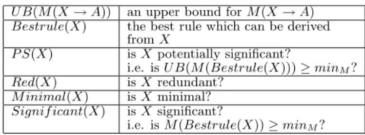
The main idea is to decide beforehand if an attribute set or its superset can produce a significant rule. If this is possible, the set is called potentially significant. Otherwise it can be pruned. Further pruning is achieved by checking the redundancy and minimality of the set. The properties are defined in Table 1.

Table 1: Properties of set X.

U B(M(X→A)) an upper bound forM(X→A)

Bestrule(X) the best rule which can be derived fromX

P S(X) isX potentially significant?

i.e. isU B(M(Bestrule(X)))≥minM?

Red(X) isX redundant?

M inimal(X) isX minimal?

Signif icant(X) isX significant?

i.e. isM(Bestrule(X))≥minM?

Now we can classify setX as

1. potentially significant (P S(X) = 1). This means that

Y ⊇X can be significant.

1.1 significant (Signif icant(X) = 1)

1.1.1 redundant (Red(X) = 1). The rule is not output. Y ) X can still be non-redundant and the search continues.

1.1.2 non-redundant (Red(X) = 0). The rule is output. Y )X can still be more significant and the search continues.

1.1.2.1 minimal (M inimal(X) = 1). Now all

Y ) X will be redundant and can be pruned.

1.1.2.2 non-minimal (M inimal(X) = 0). The search continues.

1.2 insignificant (Signif icant(X) = 0). The rule is not output. Y ) X can still be significant and the search continues.

2. not potentially significant (P S(X) = 0). This means that allY ⊇X are insignificant andY ⊇Xis pruned.

3.2 Potential significance

PropertyP S is based on estimating an upper bound for the M-value of the best rule which can be derived from a set or its specializations. It turns out that P S is anti-monotonic in most respects, meaning that if a superset of

X is P S, then X is also. For any potentially significant (l+ 1)-setY =A1...Al+1there can be at most onel-subset X = A1...Ai−1, Ai+1...Al which is not potentially

signifi-cant. This is expressed in the following theorem from [3]. Theorem 1. LetM(f r, γ)be like before. LetM ina(X)∈

X be the least frequent attribute in set X, i.e. P(M ina)≤

P(Ai)for allAi∈X. Then for any attribute setsY,X⊆Y

(i)U B(M(Bestrule(X))) =M(P(X),(P(M ina))−1₎_{, and}

(ii) IfP(M ina(X))≤P(M ina(Y)), then

U B(M(Bestrule(Y))) =M(P(X),(P(M ina(X)))−1₎_. In practice this means that an (l+ 1)-set has the same upper bound for lift as l of its parent sets have. Only one

(3)

parent set has a different least frequent attribute and pos-sibly a different upper bound for lift. When the sets are constucted in a certain order, we can guarantee that the up-perbounds for both frequency and lift (and thus forM) can only decrease.

3.3 Enumeration tree

The pruning principles can be implemented efficiently in a special kind of an enumeration tree.

A complete enumeration tree lists all attribute sets in power set P(R). In practice, it can be implemented as a trie, where each root–node path corresponds to an item set. The same structure can be used to represent the whole data set compactly. Figure 1 shows a complete enumeration tree for attribute setR={A, B, C, D, E}and a representation of an example data set. In [2] such a representation is called a

partial support tree, because the frequencies of attribute sets are only partially counted. However, the tree already con-tains all the information needed for counting the frequency of any attribute set in the complete enumeration tree.

E E E D E E E E 10 E D 1 10 A C 65 5 60 20 11 D E C B 35 E D E 5 D 5 20 D E B E E E D C ₃₅ D E C

Figure 1: A complete enumeration tree (dash line) and a tree for the example data set (solid line).

The algorithm uses an enumeration tree, where the at-tributes are ordered into descending order by their frequen-cies. Now each (l+ 1)-setXhas one parent node with a bet-ter or equal upper bound for the lift. If this special parent happens to be non-P S, thenX (which has lower frequency) is also non-P S.

If we traverse the tree in a depth-first manner from right to left, thenP(M ina(Y))≥P(M ina(X)) for allY )Xand Theorem 1 can be used for pruning. The following observa-tions tell us how we can use information from the processed subtrees for further pruning. The idea is to constructP S -candidates for theith subtree as intersections of P S-nodes in the processed subtrees on the right.

Observation 1. Let A1 ¹. . . ¹Ak be an order on

at-tributes such thatP(A1)≤. . .≤P(Ak). Lett be an

enu-meration tree, where all labels are ordered. Let t1, . . . , tk

denote the main subtrees with labelsA1, . . . , Ak. Let N(ti)

denote the set of all sets described byti;P SS(ti)⊆N(ti)the

set of potentially significant sets; and M SS(ti) ⊆P SS(ti)

the set of minimal significant sets in ti. Then for all Ai,

i < j≤k,P SS(ti)⊆ {Ai} ×(P SS(tj)\M SS(tj)).

This result means that all nodes whose counterparts in right subtrees are missing, non-P S, or minimal, can be re-moved fromti. On the other hand, we have to add some of

the nodes which are missing from ti, but which were

non-minimal andP S in all right subtrees. However, not all of

such nodes are needed. The following observation gives an extra pruning condition:

Observation 2. Letti,j be thejth subtree ofti. Then

P SS(ti,j−1)⊆(P SS(tj−1)\M SS(tj−1))∩(P SS(ti,j)\M S(ti,j)).

In practice, this means that we can take an intersection of allP Snodes in the previously processed subtrees (on the right) and right sister branches. Minimal nodes can also be removed, because more special sets could produce only redundant rules. The proofs are given in Appendix B.

4. ALGORITHM

The main idea of DeepClue is to generate an ordered enumeration tree in a top-down manner, from left-to-right. When we proceed deeper in a branch, the frequency can only decrease and the upperbound for the lift remains the same. When we move to the left subtrees, the upperbound for the lift can only decrease, and since all P S sets have one parent set on the right, we also have an upperbound for the frequency. These together define an upperbound for

M(BestRule(Y)),Y ⊇X, when setX is processed. The pseudocode is given in Figures 2 and 3. In addition, we need auxiliary functionUpdateNodes(t1, t2, t3), which implements Observations 1–2. It adds all potentially signif-icant but non-minimal sets in processed subtrees t2∩t3 to t1 and removes others.

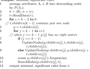
Figure 2: Algorithm DeepClue(R, r, minM) for

searching all minimal, significant association rules from data.

Input: set of attributesR, data setr, thresholdminM

Output: minimal, significant rules

1 arrange attributesAi∈Rinto descending order

byP(Ai);

2 k=|R|;n=|r|; 3 t=ReadData(r); 4 fori=k−2to0

//t.children[k−1]contains just one node

5 p=t.children[i];

6 forj=k−1toi+1

// when j==k−1p.[j]has no right sisters

7 if(j==k−1)

8 UpdateNodes(p.children[j], t.children[j], t.children[j]);

9 elseUpdateNodes(p.children[j], p.children[j+ 1], t.children[j]);

10 countp.children[j]’s frequencies; 11 SearchRules(p.children[j], t); 12 output minimal, significant rules fromt;

5. EXPERIMENTAL RESULTS

The algorithm was tested with six different data sets, us-ing two minimum confidences for each set. The goal was to find both strong rules and significant correlations, i.e. good association rules for both predictive and descriptive pur-poses. The results were compared to association rules which

(4)

Figure 3: Algorithm SearchRules(p, t) for searching rules in subtreep.

Input: nodep, root of the whole treet

Output: modified subtreep

1 if(P S(p.set) == 0) 2 p.f lag=nP S

3 else

4 ifM inimal(Bestrule(p.set))p.f lag=best; 5 else ifRed(Bestrule(p.set))p.f lag=red; 6 if(p.f lag==P S) // proceed top’s children

7 fori=k−1to0

8 SearchRules(p.children[i], t)

9 if((p.minawas changed)and(P S(p.set) == 0) 10 p.f lag=nP S; break;

11 fori= 0toi=ind−1 12 prunep’s left sisters 13 if(q.f lag==nP S) removeq

14 elseremove fromq all nodes withf lag==nP S;

were searched by traditional means, i.e. using a frequency-based pruning and selecting the best rules by different mea-sures in the post-processing phase.

The data sets and test parameters are described in Table 2. The first five data sets are biological/medical.Chessdata set was included, because it is extremely dense and contains many negative dependencies (inChessonly about 6% of all frequent rules express positive dependencies; with higher

minf r even less). All data sets and the source code can

be accessed on http://www.cs.helsinki.fi/u/whamalai/ datasets.html.

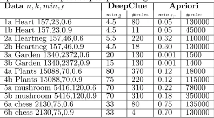
The numbers of discovered non-redundant rules are given in Table 2 and a summary of quality assessment is repre-sented in Table 3. The results were similar to our previ-ous research [3]. DeepClue discovered substantially smaller number but better quality rules than the traditional frequency-based pruning with postprocessing. The most difficult set for the classical approach was Chess, where nearly all dis-covered rules expressed independencies or negative depen-dencies. Therefore, it was also difficult to find any non-redundant significant rules.

Computationally, DeepClue turned out to be quite effi-cient. All data sets could be handled without any minimum frequency thresholds or restrictions on rule length. The maximal execution time (on Chess) was 70s. Traditional Apriori was relatively much slower (with respect to large minimum thresholds), due to a breath-first strategy and the lack of on-line redundancy reduction. The large minimum frequencies for the Apriori are partly due to heavy postpro-cessing. For feasibility, the thresholds were set to avoid over 500 000 rules. However, the dense data sets are difficult for Apriori even without this restriction. For example, Apriori cannot handleChesswithminf r<0.50.

6. CONCLUSIONS

Dependency analysis is an important but computationally demanding problem in all empirical science. It is especially problematic in bioinformatics, where data sets are often high dimensional, dense and/or strongly correlated.

Table 2: Description of tests: test number, data set, parameters, and number of rules for DeepClue and Apriori with separate postprocessing.

Datan, k, mincf DeepClue Apriori

minZ #rules minfr #rules

1a Heart 157,23,0.6 4.5 80 0.05 130000 1b Heart 157.23.0.9 4.5 11 0.05 45000 2a Heartneg 157,46,0.6 5.5 220 0.32 110000 2b Heartneg 157,46,0.9 4.5 18 0.30 130000 3a Garden 1340,2372,0.6 20 130 0.001 1500 3b Garden 1340,2372,0.9 15 130 0.001 1400 4a Plants 15088,70,0.6 80 370 0.12 18000 4b Plants 15088,70,0.9 75 220 0.12 115000 5a mushroom 5416,120,0.6 70 310 0.22 78000 5b mushroom 5416,120,0.9 70 310 0.18 350000 6a chess 2130,75,0.6 33 80 0.75 135000 6b chess 2130,75,0.9 33 4 0.70 130000

Searching association rules offers a feasible solution, but traditional frequency-based methods do not suit for depen-dency analysis. The discovered rules are often trivial or spurious while the most significant (low-frequency) rules are missed. As a solution we have introduced a new algorithm, which searches non-redundant association rules based on their frequency and lift. The algorithm is able to find glob-ally optimal rules without any frequency thresholds or re-strictions on the rule length. Due to dept-first strategy, it suits especially well for dense data sets.

7. REFERENCES

[1] R. Agrawal, T. Imielinski, and A. Swami. Mining association rules between sets of items in large databases. InProc. 1993 ACM SIGMOD Int. Conf. on Management of Data, pages 207–216, 1993.

[2] G. Goulbourne, F. Coenen, and P. Leng. Algorithms for computing association rules using a partial-support tree.Knowledge Based Systems, 13(2-3):141–149, 2000. [3] W. Hämäläinen and M. Nykänen. Efficient discovery of

statistically significant association rules. InICDM 2008, pages 203–212, 2008.

[4] H. Mannila. The role of information technology for systems biology. InSystems Biology: A Grand Challenge for Europe, pages 21–23. ESF, 2007. [5] A. Ziegler, O. Hartmann, I. B¨oddeker, and H. Sch¨afer.

Statistical genetics - present and future. InExploratory Data Analysis in Empirical Research. Proc. 25th Annual Conf. of the GfKL, Studies in Classification, Data Analysis and Knowledge Organization, pages 401–410. Springer Verlag, 2001.

APPENDIX

A. NUMBER OF ALL POSSIBLE

DEPEN-DENCIES

When the number of attributesk is odd, the number of all possible dependencies is

k X i=2 „ k i « 2i b_Xi/2c j=1 „ i j « .

The first sum lists all sets of 2–kattributes and their all possible value combinations. The second sum expresses in

(5)

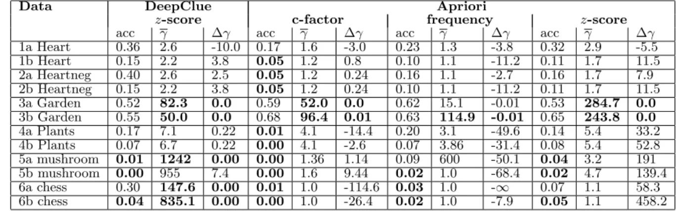
Table 3: Quality of rules for DeepClue using the z-score and Apriori using frequency, certainty factor and thez-score. For each measure, the prediction accuracy (acc), average lift (γ) and thez-score of the difference of lift (∆γ) are reported. The best results are highlighted.

Data DeepClue Apriori

z-score c-factor frequency z-score

acc γ ∆γ acc γ ∆γ acc γ ∆γ acc γ ∆γ

1a Heart 0.36 2.6 -10.0 0.17 1.6 -3.0 0.23 1.3 -3.8 0.32 2.9 -5.5 1b Heart 0.15 2.2 3.8 0.05 1.2 0.8 0.10 1.1 -11.2 0.11 1.7 11.5 2a Heartneg 0.40 2.6 2.5 0.05 1.2 0.24 0.16 1.1 -2.7 0.16 1.7 7.9 2b Heartneg 0.15 2.2 3.8 0.05 1.2 0.24 0.10 1.1 -11.2 0.11 1.7 11.5 3a Garden 0.52 82.3 0.0 0.59 52.0 0.0 0.62 15.1 -0.01 0.53 284.7 0.0 3b Garden 0.55 50.0 0.0 0.68 96.4 0.01 0.63 114.9 -0.01 0.65 243.8 0.0 4a Plants 0.17 7.1 0.22 0.01 4.1 -14.4 0.20 3.1 -49.6 0.14 5.4 33.2 4b Plants 0.07 6.7 0.22 0.00 4.1 -2.6 0.07 3.86 -31.4 0.08 5.4 52.8 5a mushroom 0.01 1242 0.00 0.00 1.36 1.14 0.09 600 -50.1 0.04 3.2 191 5b mushroom 0.00 955 7.4 0.00 1.6 9.44 0.02 1.0 -68.4 0.02 4.7 139.4 6a chess 0.30 147.6 0.00 0.01 1.0 -114.6 0.03 1.0 -∞ 0.07 1.1 58.3 6b chess 0.04 835.1 0.00 0.00 1.0 -26.4 0.02 1.0 -7.9 0.05 1.1 458.2

how many ways we can divide i attributes to two parts. With some algebraic manipulation, the equation becomes 5k

2 −3

k₊1

2. (For even values ofk, the derivation is more complex.)

B. PROOF FOR OBSERVATION 1

Proof. First we note thatN(ti) =∪kj=i+1{Ai} ×N(tj)

(Figure 1).

P SS(ti)⊆ {Ai} ×P SS(tj) follows directly from Theorem

1. SetM SS(tj) contains all minimal significant sets, i.e. the

corresponding rules have already the maximal possibleM -value, and their supersets could be only redundant. Thus, all minimal, significant sets can be found in{Ai} ×(P SS(tj)\

M SS(tj)).

C. PROOF FOR OBSERVATION 2

The idea is represented in the Figure 4.

t_j t_i,_j) U ) t_{j −1} PSS( PSS( PSS(t₋₁) j t_j) PSS( Aj j−1 A ... Ai Aj j A Aj−1 N(t )j ) ) tj t_i ) PSS( PSS( −1 j , PSS( PSS(t_{i, j}) j A

Figure 4: Potentially significant sets in branch

AiAj−1 (P SS(ti,j−1)) are a subset of potentially

sig-nificant sets in branch Aj−1 (P SS(tj−1)) and branch AiAj (P S(ti,j)).

D. NODE RECORDS

DeepClue uses an enumeration tree, where each node p

contains the following fields:

• setthe item set (in practice, we need to store only the last attribute);

• f r frequencyP(p→set);

• children[0, .., k−1] pointers to p’s children nodes (a fixed size table is used only for clarity; in practice we use a dynamic table with a separate table for labels); • f lag={nP S, P S, red, best}status ofp→set; not

po-tentially significant, popo-tentially significant, redundant or minimal;

• minathe least frequent attribute which can occur in

p’s subtree (updated, when nodes are deleted); • maxM M(Bestrule(p→set)), if pis non-redundant,

and max{q → maxM | qisp’s parent}, otherwise. This enables fast redundancy checking.